Printed version ISSN 0001-3765 / Online version ISSN 1678-2690 http://dx.doi.org/10.1590/0001-3765201820170569
www.scielo.br/aabc | www.fb.com/aabcjournal
Modeling of stem form and volume through machine learning
ANA B. SCHIKOWSKI¹, ANA P.D. CORTE², MARIELI S. RUZA², CARLOS R. SANQUETTA² and RAZER A.N.R. MONTAÑO³
¹Klabin S.A., Avenida Brasil, 26, Harmonia, 24275-000 Telêmaco Borba, PR, Brazil ²Departamento de Ciências Florestais, Universidade Federal do Paraná, Avenida Prefeito
Lothário Meissner, 632, Jardim Botânico, 80210-170 Curitiba, PR, Brazil
³Departamento de Informática, Universidade Federal do Paraná, Rua Coronel Heráclito dos Santos, 100, Centro Politécnico, Jardim das Américas, 81531-980 Curitiba, PR, Brazil
Manuscript received on September 4, 2017; accepted for publication on February 19, 2018
ABSTRACT
Taper functions and volume equations are essential for estimation of the individual volume, which have consolidated theory. On the other hand, mathematical innovation is dynamic, and may improve the forestry modeling. The objective was analyzing the accuracy of machine learning (ML) techniques in relation to a volumetric model and a taper function for acácia negra. We used cubing data, and fit equations with Schumacher and Hall volumetric model and with Hradetzky taper function, compared to the algorithms: k nearest neighbor (k-NN), Random Forest (RF) and Artificial Neural Networks (ANN) for estimation of total volume and diameter to the relative height. Models were ranked according to error statistics, as well as their dispersion was verified. Schumacher and Hall model and ANN showed the best results for volume estimation as function of dap and height. Machine learning methods were more accurate than the Hradetzky polynomial for tree form estimations. ML models have proven to be appropriate as an alternative to traditional modeling applications in forestry measurement, however, its application must be careful because fit-based overtraining is likely.
Key words: artificial intelligence, data mining, random forest, ANN.
Correspondence to: Marieli Sabrina Ruza E-mail: [email protected]
INTRODUCTION
Precision and accuracy in the quantitative analysis of measuring individual volume of forest with commercial purposes are crucial; and cubing is the most used method for this purpose. Since the quantification by cubing is expensive, due to the time and cost spent, indirect methods such as sharpening functions are usually applied for its
estimation. Functions of tapering, volume equations and form factor are commonly developed to assess the merchantable tree volumes (Clutter 1980), and are increasingly used in recent global studies of forest productivity (Liang et al. 2016).
inductive reasoning, which is based on the process of function approximation from the knowledge acquired (Faceli et al. 2011).
The nearest neighbor algorithm is the simplest of all ML algorithms, and is based on the classification or estimation of a particular attribute considering the distance of k nearest neighbors (Faceli et al. 2011). It is also instrument to estimate non-existent values in databases, besides being versatile, flexible, and simple and not having to meet the regression assumptions (Sanquetta et al. 2015b).
The RF algorithm composes a group of randomly trained regression trees, dividing explanatory variables according to their equality and inequality (Wang and Witten 1996, Breiman 2001). However, it has the disadvantage of difficult understanding about its predictive capacity and also about the impossibility of analyzing parameters (Moreno-Fernández et al. 2015).
ANNs are computational models based on the functioning of human brain, Haykin (2001) defines ANN as a processor structured by parallel distributed and interconnected units aiming at archiving knowledge, and then generalizing to an unexplored database.
The Random Forest technique has limited applications in forest research, but has seen increased applications in recent studies (Liang et al. 2016). In comparison, the k-NN are mostly used in remote sensing studies, since ANNs are more widely diffused in forest modeling in comparison to the other algorithms cited (Tatsumi et al. 2015, Were et al. 2015).
Realizing that such methods still require baselines and basic studies for the forest area, it is indispensable to evaluate them, in order to progress the efficiency in the forest modeling, focusing on the reliability of population estimators. Therefore, the aim of the present work is to evaluate the accuracy of ML, Random Forest, ANN and k nearest neighbor techniques and to compare them
to a traditional volumetric model and a tapering function for Acacia mearnsii De Wild in order to evaluate the probability of predictions improvement through machine learning techniques.
MATERIALS AND METHODS
Acacia mearnsii De Wild., popularly known as acacia negra (black wattle). Plantations are located in the state of Rio Grande do Sul (RS), segmented in three regions: Piratini, Cristal and Encruzilhada do Sul.
The planting areas have humid subtropical Cfa climate classified according to Köppen. Rains are distributed throughout the year, but with greater occurrence in summer. Average temperature in the coldest month is less than 18 ºC and higher than 22 ºC in the hottest month, with few frosts and hot summers (Brasil 1992).
We sampled four stands in each of the regions so as to include all crop rotation (10 years). In Cristal 1, 2, 5 and 10-year old stands were sampled; 1, 2, 5 and 9-year old stands in Piratini, and 1, 3, 5 and 10-year old stands in Encruzilhada do Sul.
In each stand, four circular plots with 10 m diameter were randomly installed; and tree diameters were measured at 1.30 m above the ground.
Subsequently, 683 trees were cut for rigorous cubing by the Huber method, measuring diameters relative to 5%, 15%, 25%, 35%, 45%, 55%, 65%, 75%, and 85%. 95% total stem height, totaling 10 sections.
We used 60% of database for training of algorithms and 40% for the models validation. This separation was elaborated by considering the fraction of trees by age class.
Fitting Shumacher and Hall (1933) model (Equation 1) was performed using model and reg tool in the software SAS (2002), in order to confirm regression assumptions.
( )
0 1ln(
)
2ln( )
istudy. We repeated this process 10 times, applying a different distribution at each time and fitting the model during the tests.
Age, dap, total height and relative height were used as explanatory variables for diameter estimate along the stem.
ML models were trained to obtain the volume also with the variables age, dap, total height and relative height, but logic of accumulated volume at a given relative height was used, according to Equation 3.
0
Nt
i i i
i
v
g L
=
=
∑
(3)where:
vi = stem volume at height i (m³); gi = cross-sectional area of wood pieces measured (m²); Li = length of wood pieces measured in the cubing (m); Nt = number of wood pieces.
K NEAREST NEIGHBOR
K nearest neighbors of each instance are defined according to the metrics selected, Equation 4 shows the Euclidean distance, which is commonly used for the algorithm application (Witten et al. 2011). In order to eliminate the influence of the variables scale, they were normalized according to Equation 5.
(
)
(
)
21 ,
n
i j
i
d p q p q
=
=
∑
− (4)where:
d=Euclidean distance between two points p(p1, p2,...pn) and q(q1, q2,...,qn) p and q = different individuals with n attributes or explanatory variables.
min (max min )
i i i i i v v a v v − =
− (5)
where:
ai = normalized instance; vi= current value of instance i to be normalized; max vi and min vi = maximum and minimum values of attribute i. where:
Ln = Naperian logarithm; v = stem volume (m3); βn = model coefficients; dap = diameter at 1.30 m above the ground (cm); ht = total height (m); εi = random error inherent to the regression.
The model presented by Hradetzky (1976) (Equation 2) was used for fitting the tapering function. Thus, exponents were selected by
stepwise procedure, considering 15% significance (α = 0.15) in the F test of each partial coefficient in the model, using Proc reg in the SAS software (2002). The exponents used were 0.005; 0.01; 0.02; 0.03; 0.04; 0.05; 0.06; 0.07; 0.08; 0.09; 0.1; 0.2; 0.3; 0.4; 0.5; 0.6; 0.7; 0.8; 0.9; 1; 2; 3; 4; 5; 10; 15; 20 and 25.
1 2
0 1 2
p p pn
i i i i
n i
d h h h
dap β β ht β ht β ht ε
= + + +…+ +
(2)
where:
di = diameter i along the stem (cm); dap = diameter at 1.30 m above the ground (cm); hi = height i along the stem (m); ht = total height (m); βn = model coefficients; pn = exponent selected to the model; εi = random error inherent to the regression.
Volume was estimated by the Poly Hradetzky Vi formula, incorporated into Florexel (Arce et al. 2000).
We chose stratification based on the diameter class. For fitting volume and tapering function, data were divided into 3 classes: 5 cm bellow the dap; 5 to 10 cm and over 10 cm.
Three machine-learning algorithms were analyzed: k nearest neighbor (k-NN), Random Forest (RF) algorithm, and Artificial Neural Networks (ANN).
Aha (1992) established the concept of attribute weighting, thus avoiding bias in the estimation that noise data can induce. Thus, the instance to be estimated is obtained according to its distance from the test examples (Equation 6).
1
1
* ( ) ( )
ˆ
k
i i
i
q k
i i
w f x f x
w
=
=
=
∑
∑
(6)where:
q
ˆf(x )= unknown value instance to be estimated; f(xi)= observed instances used as basis for estimation; wk = weighting factor or weight relative to the k neighbor; k = number of neighbors used in the prediction.
In this work, weighting of k nearest neighbors was standardized as the inverse of their respective distances (1/d). This method is recommended by Bradzil et al. (2003) and Sanquetta et al. (2013).
Thus, input configurations for this algorithm in the Weka software were: 20 near neighbors with activated, cross-validation weighting of distances by 1/d and linear search by the near neighbor using the Euclidean distance.
RANDOM FOREST
The RF algorithm is limited in its input parameters. Defaultsettings of Weka software were maintained, except for the number of trees to be created, since the program suggests the structuring of 100 regression trees, but Were et al. (2015) suggest that higher numbers may provide more stable results. Thus, 1,000 regression trees were constructed.
ARTIFICIAL NEURAL NETWORKS
The Weka software uses sigmoidal logistic function as activation (Equation 7), varying from 0 to 1, being then required that data to be normalized to that scale.
( )
-1
1 x
f x
e =
+ (7)
The following input parameters were provided to the Weka for ANN training: momentum 0.4 and number of times 1,000, all as fixed terms.
Regarding the learning rate and the number of neurons in the hidden layer, these were obtained using the CV Parameter Selection tool available in Weka, where it is possible to optimize parameters of algorithms. For some parameters, we used literature values due to the high computational demand.
We used only one hidden layer, since according to the Universal Approximation Theorem, only one hidden layer is enough for a MLP network to approximate any continuous function (Haykin 2001).
MODELS EVALUATION
Results obtained by models were evaluated according to the Pearson correlation (r) between the observed and predicted values, square root of the mean error (SRME%) in percentage, graphical analysis of absolute residuals and frequency histogram of percentage errors by classes in order to ratify the ranking decision, as well as identifying possible trends along the estimate line.
Additional statistics were used to complement taper models’ accuracy test, which are based on tests on the residues according to the methodology indicated by Parresol et al. (1987) and Figueiredo Filho et al. (1996).
Among them were used: deviation (D), which indicates the existence or not of tendencies between residues; Residues percentage (RP) showing the error amplitude; SQRR that relates the size of each residue to its real value, and standard deviation of differences (SD) that shows the homogeneity among residues (Parresol et al. 1987).
statistic. Therefore, the one with the lowest sum will be considered with the best performance.
RESULTS AND DISCUSSION
Table I shows coefficients fitted for Schumacher and Hall model, all coefficients being significant. Fit indicators such as the correlation between observed and predicted values and SRME% show that models are indicated for application in volume estimation. Trees below 5 cm dap were not considered in the analysis because of Weka program restriction in the fit of AI models.
Table II shows statistics for models evaluation, both for the test set used in training and fit, and for the validation set.
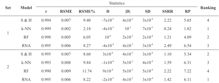
All models provided timely statistics for their use, with correlation coefficients of observed and estimated values above 0.99 and low SRMEs. As expected, test suite statistics prove more accuracy. As for the ranking of models for the training set, the three models of machine learning were more accurate than Schumacher and Hall. However, when we evaluate the validation set, we can see that these models show statistics more unstable, that is, Schumacher and Hall, and ANNs show very similar statistics in both groups, while the others do not.
The nearest neighbor algorithm (k-NN) was the best model in the test set, but it did not achieve the same success in the validation set, although its error statistics point to a technique good performance
TABLE I
Fit statistical coefficients and indicators of volumetric models fitted by dap class. Dap class
(cm) β0 β1 β2 Set R SRME%
5 a 10 -9.729** 1.898** 0.941** 1 0.977 10.088
2 0.988 7.645
> 10 -9.733**
1.853**
0.985** 1 0.988 7.827
2 0.988 7.271
Sets 1 and 2 - Training (1) and validation (2) sets; ** significant at 1%; ns not significant.
TABLE II
Fit statistics for estimation of stem total volume for training (1) and validation (2) sets.
Set Model
Statistics
Ranking
r RSME RSME% D |D| SD SSRR RP
1
S & H 0.994 0.007 9.40 -7x10⁻⁵
4x10⁻³
3x10⁻⁴
2.22 5.65 4
k-NN 0.999 0.002 2.18 -4x10⁻⁵
10-3
7x10⁻⁵
0.24 1.82 1
RF 0.998 0.005 6.05 10-4
2x10⁻³
2x10⁻⁴
1.21 4.09 2
RNA 0.995 0.006 8.27 -4x10⁻⁴
4x10⁻³
3x10⁻⁴
2.49 6.54 3
2
S & H 0.995 0.007 8.60 3x10⁻⁴
4x10⁻³
3x10⁻⁴
1.10 5.34 2
k-NN 0.993 0.008 9.84 -1x10⁻⁴
5x10⁻³
4x10⁻⁴
1.59 6.31 3
RF 0.990 0.009 11.74 9x10⁻⁴
5x10⁻³
5x10⁻⁴
2.22 7.22 4
RNA 0.995 0.006 8.22 -2x10⁻⁵
4x10⁻³
3x10⁻⁴
1.42 6.11 1
r – correlation coefficient between observed and estimated values; RSME – Absolute Root Mean Square Error; RSME% - Percentual Root Mean Square Error; D – mean deviation; |D| – mean absolute deviation; SD – standart deviation of the differences;
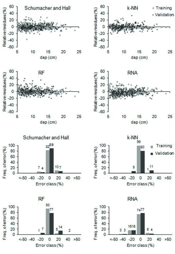
(Figure 1), where bias in the test set is extremely subtle and very close to zero.
On the other hand, both the Schumacher and Hall model and ANN (when properly trained) have the characteristic of modeling, although ANN is less explicit and more flexible due to the high number of neurons.
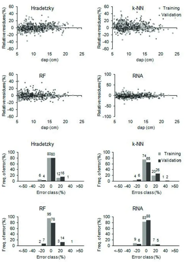
Figure 1 also shows that models did not present extreme residues, with their respective error frequencies between ± 20% center classes. It should be noted here a slight tendency of ANN to underestimate volumes, especially those of smaller magnitude.
Silva et al. (2009) states that ANNs have similar or superior accuracy to the regression models and that it still has the advantage of generalization and plasticity that allows the use of only one network to predict the volume of trees from different sites and clones.
Gorgens et al. (2014) report promising results with the use of ANNs trained with the back propagationalgorithm, suggesting that the network is constructed with more than 10 neurons in the first layer, as well as recommending the use of more than one intermediate layer. However, the network optimization did not obtain a complex model as the best result in this work, since the network considered as the one with the best performance has 3 neurons in the intermediate layer.
Özçelik et al. (2010) follow the same result line as the simplicity of ANN trained with intermediate layer and 2 or 3 neurons. They emphasize as advantage that ANNs can assimilate relations between variables through connections of their respective weights, enabling networks to model systems with complex nonlinear relationships.
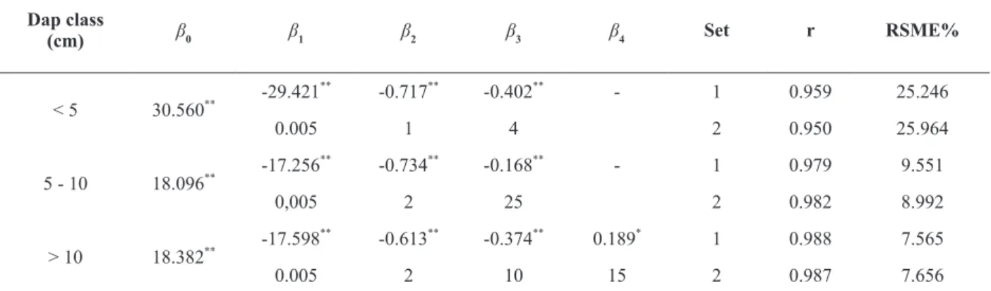
Table III shows coefficients and their respective exponents selected by the stepwise method, all coefficients being significant at 95% probability. Fitting indicators such as the correlation between observed and predicted values and SRME% demonstrate that models are suitable for use in estimating stem form. The model has greater difficulty in expressing form in individuals in the class of dap smaller than 5 cm.
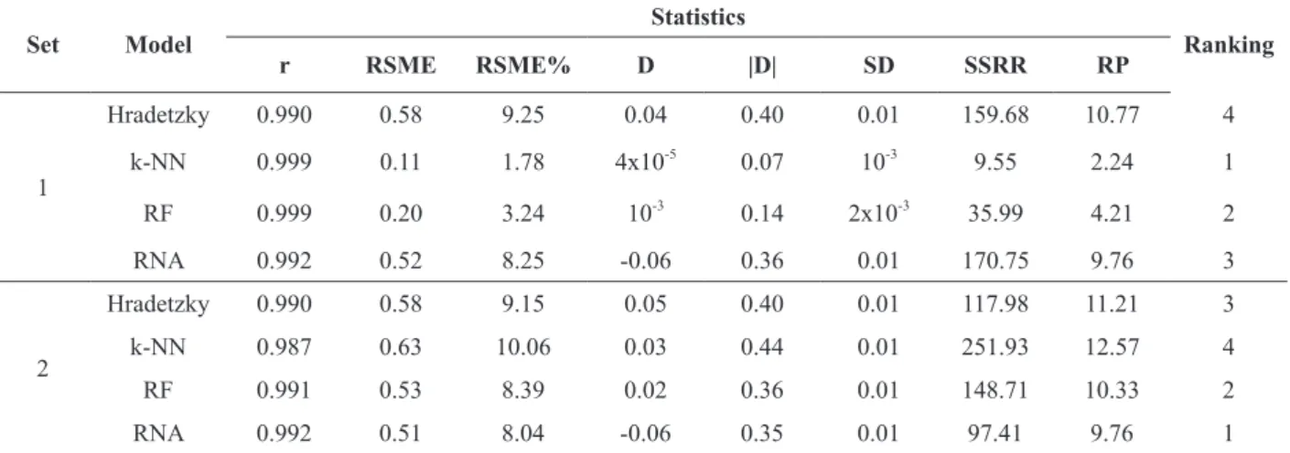
Table IV shows evaluation statistics of models, both for the test group used in training and fit, as well as for the validation group.
All models provided favorable statistics for their use, with correlation coefficients higher than 0.98 and maximum SRME of 10%. In turn, SSRR statistic showed greater discrepancy between models due to their quadratic nature. As expected, the test suite statistics demonstrate greater accuracy.
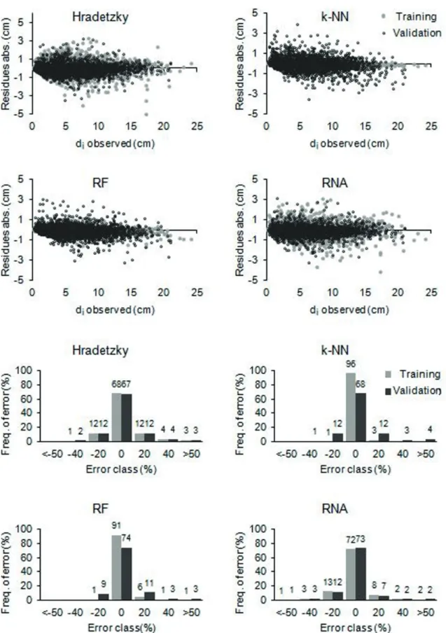
Figure 2 shows that models did not present extreme residues, with their respective frequencies of errors in ± 20% center classes.
TABLE III
Coefficients, exponents selected by stepwise and statistical indicators of taper functions fitted by dap class.
Dap class
(cm) β0 β1 β2 β3 β4 Set r RSME%
< 5 30.560** -29.421 **
-0.717**
-0.402**
- 1 0.959 25.246
0.005 1 4 2 0.950 25.964
5 - 10 18.096** -17.256 **
-0.734**
-0.168**
- 1 0.979 9.551
0,005 2 25 2 0.982 8.992
> 10 18.382** -17.598 **
-0.613**
-0.374**
0.189*
1 0.988 7.565
0.005 2 10 15 2 0.987 7.656
Sets 1 and 2 - Training (1) and validation (2) sets; * significant at 5%; ** significant at 1%; ns not significant; RSME% - Percentual
Regarding the models ranking, as well as in the estimation of the volume as function of dap and height, it is evident that even though cross validation has been applied in the training of AI models, these models may not necessarily affect good fit in the validation group. Thus, repeating here the trend of the nearest neighbor algorithm (k-NN), as the best model in the test set and worst model in the validation set.
Leite et al. (2011) compared the performance of three types of ANNs: linear perceptron, multiple layer perceptron and radial base function, with the second-degree polynomial taper function, established as Kozak’s model (1969). Authors point out that ANN models showed better fit to the database, with low values of SRME% and concentration of residues about ± 10%. However, like the present research, the models showed difficulties in the estimations of smaller diameters located in the stem’s terminal portion with strong tendencies to overestimate.
Soares et al. (2011) reported ANNs’ good performance in the estimation of relative diameters trained with the same methodology of this work, with correlation coefficients between 0.97 and 0.99, as well as SRME% values of 7% on average. As a
differential, they also point out a good accuracy of the ANNs in the prediction of recursive diameters, that is, with only 3 measures of the base in the generalization step (validation) of the model and subsequent estimation of the others. Soares et al. (2012) still propose the use of ANNs to study the form without previous knowledge of the total height, with correlation coefficients between 0.95 and 0.99, as well as mean SRME% between 1% and 20%, considering a stratification of individuals by dap class.
Table V shows evaluation statistics of the models, both for the test group used in training and fit, as well as for validation group. All models showed correlation coefficients higher than 0.98, but with SRME% values higher than those obtained in the relative diameter estimates, indicating greater variability in estimates.
Regarding the ranking, the RF model was more accurate for the training set, followed by ANN. In turn, ANN proved to be the best performing model in the validation set, followed by the Hradetzky polynomial.
Figure 3 shows the residual graphs for total volume, showing that k-NN model presented greater bias for both the training set and validation
TABLE IV
Fit statistics for diameter estimate along the stem fortraining (1) and validation (2) sets.
Set Model
Statistics
Ranking
r RSME RSME% D |D| SD SSRR RP
1
Hradetzky 0.990 0.58 9.25 0.04 0.40 0.01 159.68 10.77 4
k-NN 0.999 0.11 1.78 4x10⁻⁵
0.07 10-3
9.55 2.24 1
RF 0.999 0.20 3.24 10-3 0.14 2x10⁻³ 35.99 4.21 2
RNA 0.992 0.52 8.25 -0.06 0.36 0.01 170.75 9.76 3
2
Hradetzky 0.990 0.58 9.15 0.05 0.40 0.01 117.98 11.21 3
k-NN 0.987 0.63 10.06 0.03 0.44 0.01 251.93 12.57 4
RF 0.991 0.53 8.39 0.02 0.36 0.01 148.71 10.33 2
RNA 0.992 0.51 8.04 -0.06 0.35 0.01 97.41 9.76 1
r – correlation coefficient between observed and estimated values; RSME – Absolute Root Mean Square Error; RSME% - Percentual Root Mean Square Error; D – mean deviation; |D| – mean absolute deviation; SD – standart deviation of the differences;
set. Combined with the Hradetzky polynomial, both have a slight tendency to overestimate volumes and the k nearest neighbor has stronger bias.
RF and ANN models showed a more homogeneous distribution, with their points close to zero and showing no tendency to over- or underestimate.
Özçelik et al. (2010) indicate that ANNs implementation in forestry estimation offers several advantages over traditionally addressed methods, emphasizing that problems such as overtraining can be easily avoided with the selection of suitable architectures and use of a fit and training database. This fact was evidenced in this work, in which ANN having been proved the best model among those analyzed.
Binoti et al. (2014b) tested a method for obtaining total volume estimates with and without bark for Eucalyptus sp. using ANNs. Thus, networks were trained with clone, dap, total height and diameters related to heights 0.5, 1, 2 and 4 m, concluding that this methodology can be applied as alternative to reduce diameter measurements throughout the stem, aiming at the cubing of standing trees.
Sanquetta et al. (2015a) have tested k-NN models performance for estimating volume of
stalks of Bambusa sp., combined with fifth-degree
polynomial taper functions and Hradretzky’s fractional exponents, besides other techniques for estimation of stem volume. These authors consider that satisfactory results were not obtained with k-NN models and attribute the poor performance in the estimation to the reduced number of database. Also noting that using this technique in this case would only be indicated if linear regression premises were violated.
The Knn algorithm is versatile, simple and has great plasticity in the modeling of complex relationships. It is an important tool to estimate missing values and to explore local deviations in databases (Eskelson et al. 2009, Fehrmann et al. 2008). When compared to the traditional methods of regression, Knn algorithms has the disadvantage of not having well-studied statistical properties. Moreover, the sample size can be a limiting to accurate is preferred (Mognon et al. 2014, Haara and Kangas 2012).
The Random Forest technique does not need assumptions about data distribution, because it has high capacity to model complex interactions among a large number of predictive variables and demand no overtraining to the database (Prassad et al. 2006).
TABLE V
Fit statistics for estimation of stem total volume for training (1) and validation (2) sets.
Set Model
Statistics
Ranking
r RSME RSME% D |D| SD SSRR RP
1
Hradetzky 0.994 0.01 10.40 2x10⁻³
5x1
0-3 3x10⁻⁴
2.67 6.35 4
k-NN 0.994 0.01 10.05 10-3
5x10⁻³
3x10⁻⁴
3.29 7.20 3
RF 0.999 2x10⁻³ 2.17 3x10⁻⁴ 10-3 6x10⁻⁵ 0.85 2.97 1
RNA 0.994 0.01 9.31 10-3
4x10⁻³
3x10⁻⁴
2.30 5.95 2
2
Hradetzky 0.994 0.01 10.80 2x10⁻³
5x10⁻³
4x10⁻⁴
1.55 6.24 2
k-NN 0.989 0.01 12.64 2x10⁻³
0.01 5x10⁻⁴
3.43 8.97 4
RF 0.990 0.01 11.65 8x10⁻⁴
0.01 5x10⁻⁴
1.94 6.78 3
RNA 0.995 0.01 8.32 6x10⁻⁴
4x10⁻³
3x10⁻⁴
1.13 5.47 1
r – correlation coefficient between observed and estimated values; RSME – Absolute Root Mean Square Error; RSME% - Percentual Root Mean Square Error; D – mean deviation; |D| – mean absolute deviation; SD – standart deviation of the differences;
However, RF is not a tool for traditional statistical inference; therefore, it is not suitable for ANOVA and hypothesis tests. It does not compute p values, regression coefficients, or confidence intervals. The lack of a mathematical equation or graphical representation may hinder its interpretation (Cutler et al. 2007).
RNAs have the ability to model non-explicit characteristics among variables. In comparison to traditionally applied models, they have the advantage of generating estimates for different strata with a single model, besides the possibility of including categorical variables in their models (Gorgens et al. 2009, Silva et al. 2009 and Binoti et al. 2014a, b). The RNAs still have great adaptability, tolerance to outliers and ease of application after network training (Leite et al. 2011). As a disadvantage, they have difficulties in choosing the network configuration, requiring high computational capacity and demanding care to avoid overtraining in relation to the database.
On the other hand, regression analysis has a consolidated theory of wide application. It has the possibility of obtaining different variables of interest, being less demanding in numbers of observations with the advantage of interpreting parameters. However, the predefined curve behavior makes it difficult to properly adjust to different databases. The advantage of Artificial Intelligence remains in the ability to identify relationships between variables that are too complex for parametric models (Strobl et al. 2009).
CONCLUSION
Schumacher and Hall model and ANN showed the best results for volume estimation depending on dap and height when compared to Random Forest and k nearest neighbor.
Artificial intelligence methods used prove to be more accurate than the Hradetzky polynomial for tree form study estimates, such as the diameter along the stem and total volume.
ML models are appropriate as alternative in traditionally applied modeling in forestry measurement; however, their use should be cautious because of the greater possibility of fit-based overtraining.
REFERENCES
AHA D. 1992. Tolerating noisy, irrelevant and novel attributes in instance-based learning algorithms. Int J Man-Machine Studies 36(2): 267-287.
ARCE JE, KOEHLER A, JASTER CB AND SANQUETTA CR. 2000. Florexel – Funções Florestais desenvolvidas para o Microsoft Excel. Centro de Ciências Florestais e da Madeira (CCFM). Universidade Federal do Paraná, Curitiba, 2000.
BINOTI DHB, BINOTI MLMS AND LEITE HG. 2014a. Configuração de redes neurais artificiais para estimação do volume de árvores. Ciência da Madeira 5(1): 58-67. BINOTI MLMS, BINOTI DHB, LEITE HG, GARCIA SLR,
FERREIRA MZ, RODE R AND SILVA AAL. 2014b. Redes neurais artificiais para estimação do volume de árvores. Rev Árvore 38(2): 283-288.
BRADZIL P, SOARES CC AND JOAQUIM P. 2003. Ranking Learning Algorithms: Using IBL and Meta-Learning on Accuracy and Time Results. Mach Learn 50: 251-277. BRASIL. 1992. Ministério da Agricultura e Reforma Agrária.
Secretaria Nacional de Irrigação. Departamento Nacional de Meteorologia. Normas climatológicas (1961-1990). Brasília, 84 p.
BREIMAN L. 2001. Random Forests. Mach Learn 45(1): 5-32.
CLUTTER JL. 1980. Development of taper functions from variable-top merchantable volume equations. Forest Sci 26(1): 117-120.
CUTLER DR, EDWARDS TC, BEARD KH, CUTLER A, HESS K, GIBSON J AND LAWLER J. 2007. Random forests for classification in ecology. Ecology 88: 2783-2792.
ESKELSON BNI, TEMESGEN H, LEMAY V, BARRETT TM, CROOKSTON NL AND HUDAK T. 2009. The roles of nearest neighbor methods in imputing missing data in forest inventory and monitoring databases. Scand J For Res 24: 235-246.
FACELI K, LORENA AC, GAMA J AND CARVALHO ACPLF. 2011. Inteligência artificial: uma abordagem de aprendizado de máquina. Rio de Janeiro, LTC, 378 p. FEHRMANN L, LEHTONEN A, KLEINN C AND TOMPPO
E. 2008. Comparison of linear and mixed-effect regression models and a k-nearest neighbor approach for estimation of single-tree biomass. Can J For Res 38(1): 1-9.
GORGENS EB, LEITE HG, GLERIANI JM, SOARES CPB AND CEOLIN A. 2009. Estimação do volume de árvores utilizando redes neurais artificiais. Rev Árvore 33(6): 1141-1147.
GORGENS EB, LEITE HG, GLERIANI JM, SOARES CPB AND CEOLIN A. 2014. Influência da arquitetura na estimativa de volume de árvores individuais por meio de redes neurais artificiais. Rev Árvore 38(2): 289-295. HAARA A AND KANGAS A. 2012. Comparing k nearest
neighbors methods and linear regression – is there reason to select one over the other? Mathematical and Computational Forestry & Natural-Resource Sciences 4(1): 50-65.
HALL M, FRANK E, HOLMES G, PFAHRINGER B, REUTEMANN P AND WITTEN IH. 2009. The WEKA Data Mining Software: An Update. SIGKDD Explorations 11(1): 10-18.
HAYKIN SS. 2001. Redes neurais: princípios e prática. Tradução Paulo Martins Engel. 2ª ed., Porto Alegre, Bookman, 900 p.
HRADETZKY J. 1976. Analyse und interpretation statstisher abränger keiten. (Biometrische Beiträge zu aktueller forschungs projekten). Baden: Württemberg Mitteilungen der FVA, 146 p.
KOZAK A, MUNRO DD AND SMITH JGH. 1969. Taper functions and their applications in forest inventory. For Chron 45(4): 278-283.
LEITE HG, SILVA MLM, BINOTI DHB, FARDIN L AND TAKIZAWA FH. 2011. Estimation of inside-bark diameter and heartwood diameter for Tectona grandis Linn. trees using artificial neural networks. Eur J Forest Res 130(2): 263-269.
LIANG J ET AL. 2016. Positive biodiversity-productivity relationship predominant in global forests. Science 354(6309): aaf8957.
MOGNON F, CORTE APD, SANQUETTA CR, BARRETO TG AND WOJCIECHOWSKI J. 2014. Estimativas de biomassa para plantas de bambu do gênero Guadua. Rev Ceres 61(6): 900-906.
MORENO-FERNÁNDEZ D, CAÑELLAS I, BARBEITO I, SÁNCHEZ-GONZÁLEZ M AND LEDO A. 2015. Alternative approaches to assessing the natural regeneration of Scots pine in a Mediterranean forest. Ann For Sci 72(5): 569-583.
ÖZÇELIK R, DIAMANTOPOULOU MJ, BROOKS JR AND WIANT JUNIOR HV. 2010. Estimating tree bole volume using artificial neural network models for four species in Turkey. J Environ Manage 91(3): 742-753.
PARRESOL BR, HOTVEDT JE AND CAO QV. 1987. A volume and taper prediction system for bald cypress. Can J Forest Res 17: 250-259.
PRASAD AM, IVERSON LR AND LIAW A. 2006. Newer Classification and Regression Tree Techniques: Bagging and Random Forests for Ecological Prediction. Ecosystems 9(2): 181-199.
SANQUETTA CR, SANQUETTA MNI, CORTE APD, PÉLLICO NETTO S, MOGNON F, WOJCIECHOWSKI J AND RODRIGUES AL. 2015a. Modeling the apparent volume of bamboo culms from Brazilian plantation. Afr J Agric Res 10(42): 3977-3986.
SANQUETTA CR, WOJCIECHOWSKI J, CORTE APD, BEHLING A, PÉLLICO NETTO S, RODRIGUES AL AND SANQUETTA MNI. 2015b. Comparison of data mining and allometric model in estimation of tree biomass. BMC Bioinformatics 16: 247.
SANQUETTA CR, WOJCIECHOWSKI J, CORTE APD, RODRIGUES AL AND MAAS GCB. 2013. On the use of data mining for estimating carbon storage in the trees. Carbon Balance Manag 8: 6.
SAS INSTITUTE INC. 2002. SAS/STAT User’s Guide, Version 9.2. SAS Institute: Cary Inc.
SCHUMACHER FX AND HALL FS. 1933. Logarithmic expression of timber-tree volume. J Agric Res 47(9): 719-734.
SILVA MLM, BINOTI DHB, GLERIANI JM AND LEITE HG. 2009. Ajuste do modelo de Schumacher e Hall e aplicação de redes neurais artificiais para estimar volume de árvores de eucalipto. Rev Árvore 33(6): 1133-1139. SOARES FAAMN, FLÔRES EL, CABACINHA CD,
CARRIJO GA AND VEIGA ACP. 2011. Recursive diameter prediction and volume calculation of Eucalyptus trees using multilayer perceptron networks. Comput Electroni Agric 78(1): 19-27.
SOARES FAAMN, FLÔRES EL, CABACINHA CD, CARRIJO GA AND VEIGA ACP. 2012. Recursive diameter prediction for calculating merchantable volume of Eucalyptus clones without previous knowledge of total tree height using artificial neural networks. Applied Soft Computing 12: 2030-2039.
STROBL C, MALLEY J AND TUTZ G. 2009. An introduction to recursive partitioning: rationale, application and characteristics of classification and regression trees, bagging and random forests. Psychol Methods 14: 323-348.
TATSUMI K, YAMASHIKI Y, TORRES MAC AND TAIPE CLR. 2015. Crop classification of upland fields using Random forest of time-series Landsat 7 ETM+ data. Comput Electron Agric 115: 171-179.
WANG Y AND WITTEN IH. 1996. Induction of model trees for predicting continuous classes. Working Paper 96/23. WERE K, BUI DT, DICK OB AND SINGH BR. 2015. A
comparative assessment of support vector regression, artificial neural networks, and random forests for predicting and mapping soil organic carbon stocks across an Afromontane landscape. Ecol Indic 52: 394-403. WITTEN IH, EIBE F AND HALL MA. 2011. Data mining:
practical machine learning tools and techniques. 3rd