Discrete Optimization
A node rooted flow-based model for the local access network expansion problem
Margarida Corte-Real
a,*, Luís Gouveia
baFEG, Universidade Católica Portuguesa, Rua Diogo Botelho, 1327, 4169-005 Porto, Portugal bCIO and DEIO, F.C., Universidade de Lisboa, Bloco C6, Piso 4, 1749-016 Lisboa, Portugal
a r t i c l e
i n f o
Article history:
Received 31 March 2009 Accepted 2 October 2009 Available online 12 October 2009
Keywords:
Network flows Local access network
Capacitated Minimum Spanning Tree Problem
Valid inequalities
a b s t r a c t
In this paper, we present a new formulation for the local access network expansion problem. Previously, we have shown that this problem can be seen as an extension of the well-known Capacitated Minimum Spanning Tree Problem and have presented and tested two flow-based models. By including additional information on the definition of the variables, we propose a new flow-based model that permits us to use effectively variable eliminations tests as well as coefficient reduction on some of the constraints. We present computational results for instances with up to 500 nodes in order to show the advantages of the new model in comparison with the others.
Ó2009 Elsevier B.V. All rights reserved.
1. Introduction
A local access network is composed by a set of customer nodes, a central office and several links that allow the transmission of the traffic from one customer to another through the central office. The network has a tree structure that connects the customers to the central office, located at the root of the tree. This work addresses the local access network expansion problem (LANEP), where an existing network must be adapted to traffic increase either by expanding the capacity of the links and/or by installing concentrators in some nodes. Concentrators are electronic devices that compress the traffic and can be installed in the network in order to eliminate or reduce the need of the links expansion.Balakrishnan et al. (1991)and, more recently,Carpenter and Luss (2006)have presented the main characteristics of several problems arising in the context of access network planning. Some variants of the local access network expansion problem have also been considered in the literature, with different kinds of concentrators and transmission links and for single and multi-period versions (see, for instance,Bienstock (1993), Lee (1993), Balakrishnan et al. (1995), Cho and Shaw (1996, 1998), and Flippo et al. (2000)for single-period versions of the problem andJack et al. (1992), Shulman and Vachani (1993), Gendreau et al. (2006) and Kouassi et al. (2009)for multi-period versions).
The problem we address here is the expansion of a local access network with a fixed tree topology. We consider the single time period version of the problem, where we want to determine, with minimum cost, which links need to be expanded and/or where the concentra-tors should be located in order to guarantee that the node demands can be sent to (or from) the central office. We consider the version of the problem with uncapacitated concentrators. It was shown inCorte-Real and Gouveia (2007)that the LANEP could be seen as an exten-sion of the well-known Capacitated Minimum Spanning Tree Problem (CMSTP) (see, for instance,Gavish (1993) and Gouveia and Lopes (2000)) and, as a consequence, two flow-based models were proposed and tested for the LANEP. These two models, denoted byFAand
FD, are characterized respectively by aggregated and disaggregated flows that circulate in the links and are augmented versions of models originally developed for the CMSTP. In this paper we review theFAmodel and present a new flow-based model that adds information on the first node of each feasible path in the graph (that corresponds to the central office or to a concentrator). As we shall show, this addi-tional information permits us to create a model with a linear programming relaxation that is substantially tighter than the linear program-ming relaxation of theFAmodel. Furthermore, the new information on the variables permits us to use effectively variable elimination tests as well as coefficient reduction on some of the constraints of the new model. These features lead to more solution methods for the problem which are, in general, more efficient than the ones based on the previousFAandFDmodels.
0377-2217/$ - see front matterÓ2009 Elsevier B.V. All rights reserved.
doi:10.1016/j.ejor.2009.10.001
*Corresponding author. Tel.: +351 226 196 200.
E-mail addresses:[email protected],[email protected](M. Corte-Real),[email protected](L. Gouveia).
Contents lists available atScienceDirect
European Journal of Operational Research
The paper is organized as follows. Section2defines the problem and presents the assumptions that are usually given for the problem. In Section3we review how the LANEP can be seen as an extension of the CMSTP and review the aggregated flow modelFAas well as some valid inequalities presented inCorte-Real and Gouveia (2007). We also introduce new inequalities that permit us to improve the linear programming relaxation of theFAmodel. In Section3.3we make a brief reference to the disaggregated flow modelFD. In Section4we present the new model, the Node Rooted Aggregated Flow model denoted byNRFA, and develop several sets of valid inequalities that are based on the definition of new variables and that improve considerably the linear programming relaxation of the original model. We analyse the inequalities introduced for theFAmodel and show that several of them are redundant in the linear programming relaxation of the new model. Section5gives some computational results to evaluate the efficiency of the proposed models: in Section5.1some pre-processing techniques for variables elimination and coefficient reduction are described and Section5.2presents several computational re-sults to compare the three classes of models from a set of tests with 100, 200 and 500 nodes. The last section presents some conclusions.
2. Problem description
A local access network is composed by a set of customer nodes, a central office and several links that allow the transmission of the traffic from one customer to another through the central office. The network has, in general, a fixed tree structure (neither nodes nor edges can be added) where the central office is the root of the tree and all the other nodes represent the customer nodes. Concentrators that compress the traffic can be installed in the customer nodes. The edges of the network correspond to the existent links between the customer nodes. In the local access network expansion problem, due to traffic demand increase, we need to expand the given network either through the installation of concentrators at the nodes or through the expansion of the capacity on the links. To each link we associate an available capacity that identifies the amount of information that can circulate initially on the link, a maximum capacity that corresponds to the max-imum amount of traffic that will be able to circulate on the link after expanding the network and the costs of its expansion. To each node, we associate its demand and the costs of locating a concentrator.
LetT¼ ðN;EÞbe the tree defining the local access network, letN¼ f1;. . .;ngbe the corresponding node set (node 1 is the root of the tree and represents the central office node) and letEbe the edge set of the tree (corresponding to the existing links between customer nodes). For each nodej, letdjbe the corresponding demand and letFjandcjbe, respectively, the fixed and variable costs of installing a concentrator
at that node. For each edgeði;jÞ, we associate the available capacityBijand the maximum capacityMijwhich corresponds to an upper bound
on the traffic that will be able to circulate on the edge after expanding the network (this value can be equal to the total demand of the tree). We also define a fixed costGijand a variable costeij, corresponding to the expansion of the linkði;jÞ.
Given the demand in each node, the capacities and costs related to each edge and the concentrators costs, the local access network expansion problem is to determine, with minimum cost, which edges need to be expanded and/or where the concentrators should be lo-cated in order to guarantee that the node demands can be sent to (or from) the root node. We consider the following assumptions, already stated in,Balakrishnan et al. (1995), Cho and Shaw (1996, 1998), Flippo et al. (2000) and Corte-Real and Gouveia (2007):
The information is concentrated once, either by one concentrator or by the central office (the central office can be viewed as a concen-trator with zero costs);
The demand of each node is unsplitted, that is, all the demand is processed by only a single concentrator or by the central office; If the demand of a nodeiis processed by a given concentrator, the demand of every node in the path from nodeito the concentrator is
also processed by the same concentrator (called contiguity restriction);
The demand processed by a given concentrator is transmitted to the central office through the original links of the network (and the capacity used is considered insignificant) or by a direct link to the central node (in this case, the corresponding transmission cost is incorporated in the fixed cost of the concentrator).
The problem has been extensively studied byBalakrishnan et al. (1995), which state that the problem is NP-hard. They present a method that combines lagrangian relaxation with a dynamic programming algorithm in order to generate upper and lower bounds on the optimal value of the problem. Later on,Flippo et al. (2000)presented a pseudo-polynomial dynamic programming algorithm for the problem which depends on a constant valueBthat represents an upper bound on the capacity of the concentrators. Their algorithm solves the problem in
OðnB2
Þtime andOðnBÞstorage space (wherenrefers to the size of the network) and considers more general cost structures for links expan-sion and concentrators installation. For the case with uncapacitated concentrators that we are considering, the parameterBis set equal to the total demand (as the authors of that paper suggest). The computational experience shown inCorte-Real and Gouveia (2007)gives empirical evidence that the flow-based models should be, in general, preferred when compared with the dynamic programming approach for the uncapacitated version of the problem.
3. Graph transformation and flow-based models
3.1. Graph transformation and the FA model (Corte-Real and Gouveia, 2007)
In this section, we review the approach described inCorte-Real and Gouveia (2007). With the inclusion of an additional node 0 and edgesð0;jÞfor each nodej2N(denoted byauxiliary edges), we transform the problem under study into an extension of the CMSTP. Given
the treeT, node and edge setsNandEas presented in the previous section, we define a new graphT0, obtained fromTby adding the new
node and the new edges, as described inFig. 1. LetN0denote the node set inT0and letE0denote the corresponding edge set.
When an edgeð0;jÞis included in the solution inT0, it means that a concentrator is located at nodej. The total demand served by that
concentrator inTis represented by the flow in the edgeð0;jÞinT0. Since the inclusion of each one of these edges inT0corresponds to the
installation of one concentrator inT, the corresponding available edge capacityB0jmust be unlimited and these edges are not included in
the set of edges to be expanded. Forj2N, we also define the coefficientM0jas an upper bound on the traffic that can be served by the
atj;Fj, and the other corresponding to the variable costcj, which depends on the amount of flow that circulates through the edge.Fig. 2
illustrates a feasible solution inTand the corresponding feasible solution inT0. As we can see, this solution is a spanning tree in the new graph.
The representation of the problem given by the new graph permits us to model the problem as a capacitated network flow model inT0. Since a powerful modelling construct to improve formulations for several network design problems is to ‘‘direct the given network” (see, for instance,Goemans and Myung (1993) and Magnanti and Wolsey (1995)), we model our problem in a directed graphD0¼ ðN0;A0Þ, whereN0denotes the set of nodes andA0the set of all arcs, as described next: each edgeði;jÞinE0is replaced by two arcs,hi;jiand hj;ii, with the same parameters as the original edge (the exception are edges of the formð1;jÞandð0;jÞthat are replaced only by one single
arc,h1;jiandh0;ji, respectively, since we consider that the traffic flows from the central office/concentrators to the nodes). The arcs of the formh0;ji, for each nodej2N, are designated asauxiliary arcs. The setAcorresponds to the set of arcs without the auxiliary arcs.
Based on this representation,Corte-Real and Gouveia (2007)has described an adaptation for the new problem of a single-commodity model originally proposed for the CMSTP. We define, for each archi;ji 2A0, the binary variablexijindicating whether or not the archi;jiis included in the solution and a nonnegative variableyij, indicating the amount of flow that circulates in the arc. For each archi;ji 2A, letzij
denote the binary variable indicating whether or not the archi;jiis expanded andsija nonnegative variable indicating the added capacity to
the arc. The basic directed single-commodity flow formulation, denoted byFA0, is as follows:
Minimize X
n
j¼1
Fjx0jþ
X
n
j¼1
cjy0jþ
X
hi;ji2A Gijzijþ
X
hi;ji2A eijsij
subject to X i:hi;ji2A0
xij¼1
8
j2N; ð1ÞX
i:hi;ji2A0
yij
X
i:hj;ii2A
yji¼dj
8
j2N; ð2Þzij6xij
8
hi;ji 2A; ð3Þyij6Bijxijþsij
8
hi;ji 2A; ð4Þy0j6M0jx0j
8
j2N; ð5Þsij6ðMijBijÞzij
8
hi;ji 2A; ð6Þxij2 f0;1g;yijP0
8
hi;ji 2A0; zij2 f0;1g; sijP08
hi;ji 2A: ð7ÞConstraints(1)ensure that each node, except node 0, has only one incident arc and constraints(2)are the flow conservation con-straints, guaranteeing that each nodejreceivesdjunits. Constraints(3)ensure that an arc inAis expanded only if it is used. For each
one of these arcs, constraints(4)guarantee that the flow in any arc is less or equal than the available capacity plus the added capacity. For the auxiliary arcsh0;ji, constraints(5)state that the flow value is less or equal than the maximum capacityM0j. Constraints(6)
de-fine an upper bound on the added capacity to the expanded links (the maximum demand that can circulate in the arc minus the cor-responding available capacity). The last set represents the variables domain. The objective function states that we want to minimize the sum of the concentrator costs together with the link expansion costs. Note that constraints(4) and (6)together with(3)guarantee that
Fig. 1.Structure of: (a)Tand (b)T0.
the constraintsyij6Mijxij 8hi;ji 2Aare verified and that is why they were not explicitly included. These constraints together with(5), (1), (2), and the nonnegativity constraints(7), guarantee that the set of arcs defined by thexvariables equal to 1 define a spanning tree in the graphD0.
In order to improve the optimal solution of the linear programming relaxation ofFA0, several sets of valid inequalities were described in Corte-Real and Gouveia (2007). As these inequalities are needed for comparing with some of the inequalities for the newNRFAmodel, we make a brief review of them.
As noted inCorte-Real and Gouveia (2007), subtour elimination constraints are satisfied by the solutions of the problem. In particular, the linear programming relaxation of the model was substantially improved by adding the simple 2-subtour elimination constraints:
xijþxji61
8
ði;jÞ 2E; i;j–1: ð8ÞAnother interesting class of inequalities is based on the concept of Saturated Nodes (originally introduced inBalakrishnan et al. (1995)). We recall that anode j is saturatedif the total demand in the subtree rooted at nodej, which is denoted byDðjÞ, is greater than the available capacity in the arc that connects the predecessor ofj;aj, toj. LetNsbe the set of saturated nodes and letTðjÞbe the subtree rooted at nodej.
Two sets of constraints, based on the concept of saturated nodes, are as follows:
X
k2TðjÞ
x0kþzajjP1
8
j2 Ns; ð9ÞðDðjÞ BajjÞ
X
k2TðjÞ x0k
0
@
1
AþsajjPðDðjÞ BajjÞ
8
j2Ns: ð10ÞFor each saturated nodej, constraints(9)guarantee that either we install at least one concentrator in the subtree rooted atjor we ex-pand the arc that converges into nodej; constraints(10)ensure that, if no concentrator is installed in that subtree, the expanded capacity must be greater or equal than the difference of the total demandDðjÞand the available capacity of the arc.
3.2. New inequalities – inequalities that give lower and upper bounds on the value of the arcs
In this paper, we introduce new inequalities that are lower and upper bounding inequalities on the value of the arc flows and that gen-eralize, in some sense, simple lower and upper bounding flow inequalities.
Since the value of the flow on archi;jimust satisfy at least the demand of that node, we have the following well-known lower bounding
inequalities, already used inCorte-Real and Gouveia (2007):
yijPdjxij
8
hi;ji 2A0: ð11ÞSimilar and more general inequalities, originally described inGouveia and Lopes (2000), that consider one or all the arcs diverging from nodej are also valid to the problem and were used in Corte-Real and Gouveia (2007). Here, we present stronger versions of these inequalities:
yijPðdjþdkÞxijþdkðxjkþxkj1Þ
8
hi;ji 2A0; hj;ki 2A ðk–iÞ; ð12ÞyijP djþ
X
k:hj;ki2A;k–i dk
!
xijþ
X
k:hj;ki2A;k–i
dkðxjkþxkj1Þ
8
hi;ji 2A0: ð13ÞThese inequalities differ from the versions presented inCorte-Real and Gouveia (2007) and Gouveia and Lopes (2000)due to the extraxkj
term involved in the right hand-side summation terms.
Result 3.1. Inequalities(12) and (13)are valid for the LANEP.
Proof.For simplicity we only proof the validity of(12)since the proof of(13)is similar. Since(12)is known to be valid whenxkj¼0, we
only need to address the case withxkj¼1. But then, by(1),xij¼0 andyij¼0 by constraintsyij6Mijxij 8hi;ji 2A0. The inequality becomes
xjkþxkj61 which is valid. h
It can be easily proved that the inclusion of(13)does not imply that constraints(11) and (12)become redundant in the linear program-ming relaxation ofFA0or that the inclusion of(12)implies the redundancy of(11). Thus, using both sets together with(11)might lead to better linear programming bounds and this is confirmed by our results.
We introduce, next, new inequalities that are upper bounding analogues of the previous inequalities. In order to introduce these general upper bounding inequalities, we define more precisely theMijcoefficients that appear in constraints(6). Since, for each archi;jithe cor-responding coefficient represents the maximum capacity that can circulate in archi;ji, its value can be made equal to the total demand of
the nodes that can be served through the arc (seeCorte-Real and Gouveia (2007)). If some nodes are disconnected from the arc by the elim-ination of some arcs from the graph, this coefficient value can be further reduced.
In a similar way as was previously developed for the lower bounding inequalities, we develop upper bounding inequalities related to the flow in each archi;ji. Consider the following inequalities:
yij6ðMijMjkÞxijþMjkxjk
8
hi;ji 2A0; hj;ki 2Aðk–iÞ: ð14ÞAs done previously with(12)to obtain(13), we can adapt constraints(14)in order to include all the diverging arcs from nodejleading to
yij6djxijþ
X
k:hj;ki2A;k–i
Mjkxjk
8
hi;ji 2A0: ð15ÞResult 3.2. Inequalities(14) and (15)are valid for the LANEP.
Proof. Again, we only provide the proof of the validity of(14)since the proof of(15)is similar. Consider the following three cases: (i) if
xij¼xjk¼1, we getyij6Mij, which is valid as referred before (part (a) ofFig. 3); (ii) ifxij¼1 andxjk¼0,yij6MijMjk, which is valid
because theMjkcoefficient includes the demand of all nodes of the ‘‘subtree rooted ink” and these nodes cannot be served through arc
hi;ji;MijMjk is then an upper bound on the flow value that circulates inhi;ji(part (b) ofFig. 3); (iii) ifxij¼0, we getyij¼0 from
yij6Mijxij 8hi;ji 2A0, and thusxjkP0, which is valid from the nonnegativity constraints(7). h
Similarly to what was stated before for the lower bounding inequalities, the inclusion of(15)inFA0formulation does not make(14) redundant in the linear programming relaxation ofFA0.
Finally, we can create constraints that are similar to the previously given constraintssij6ðMijBijÞzij 8hi;ji 2A(6):
sij6ðMijMjkBijÞzijþMjkxjk
8
hi;ji;hj;ki 2A ðk–iÞ; ð16Þ sij6ðdjBijÞzijþX
k:hk;ji2A;k–i
Mjkxjk
8
hi;ji 2A; ð17Þwhich consider, respectively, one or all the arcs diverging from nodej.
Result 3.3. Inequalities(16) and (17)are valid for the LANEP.
Proof. Similarly to previous results, we only prove the validity of(16). Consider the following three cases: (i) ifzij¼1 andxjk¼1, the
inequality becomessij6MijBij, which is valid due to(6); (ii) ifzij¼1 andxjk¼0, we getsij6MijMjkBij; since the archj;kiis not
in the solution, the maximum value of the flow that can circulate inhi;jiis given byMijMjk and the added capacity to the arc must
be less or equal than this maximum flow value minus the available capacity; (iii) ifzij¼0, we getsij¼0 from(6) and (7)andMjkxjk is
always nonnegative. h
The following result shows that inequalities(16) and (17)imply constraints(14) and (15), respectively. Thus, only the inequalities(14) and (15)corresponding to auxiliary arcs are considered for augmenting theFA0formulation.
Result 3.4. (i) For each archi;ji 2Aand each archj;ki 2A(withk–iÞ, inequality(16)implies inequality(14)and (ii) for each archi;ji 2A,
inequality(17)implies inequality(15).
Proof. (i) Let hi;jiand hj;kibe two arcs inA (with k–iÞ. By combining(4) for the archi;ji with(16), for hi;jiandhj;ki, we obtain yij6Bijxijþ ðMijMjkBijÞzijþMjkxjk. By combining this inequality with(3)for the samehi;ji, we obtain yij6ðMijMjkÞxijþMjkxjk as
desired. The proof of (ii) is similar. h
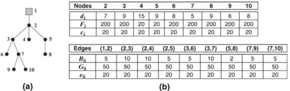
To illustrate that the inclusion of several of these valid inequalities can improve the linear programming relaxation ofFA0, we introduce the following example where a local access network with 10 nodes is considered.
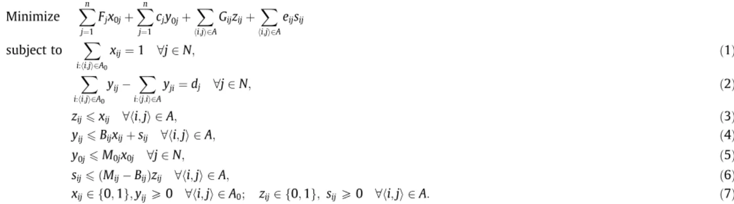
Example 3.1. Consider the local access network with 10 nodes denoted bytree 10and shown inFig. 4, whose structure is represented in (a) and the associated parameters in (b).
Table 1depicts the linear programming bound obtained withFA0formulation and the same formulation augmented with the different sets of the inequalities presented before. Several combinations were performed but, for simplicity, we have chosen the eight formulations presented in the table and easily identified by the designation at the top of each column.Table 1includes two more columns, the first one characterizes the instance considered and the last one gives the optimal cost. We have also included the results taken from the instances
tree 10_Fx2andtree 10_Bx2, obtained fromtree 10by, respectively, doubling the fixed cost of installing the concentrators and doubling the available capacity of the links.
Fig. 3.Upper bound on the flow value in archi;ji: (a)Mij, ifhj;kiis in the solution (b)MijMjk, otherwise.
The results on theTable 1show that the several sets of inequalities previously discussed improve the cost of the linear programming solution presented in column ‘‘FA0”. The second formulation represents theFA0formulation augmented with the 2-subtour elimination constraints and the constraints based on the saturated nodes. The next three show the effect of the inclusion of the lower bounding inequalities: the simple ones(11)and the more general inequalities(12) and (13). In the next two columns we include the lower and upper bounding inequalities (in the last case, the upper bounding inequalities(14) and (15)are included only for the auxiliary arcs). The last col-umn ‘‘FA1” gives theFA0formulation augmented with all the inequalities presented.
3.3. Disaggregated flow model – FD (Corte-Real and Gouveia, 2007)
We now make a brief reference to theFDmodel, the multi-commodity version of theFAmodel presented inCorte-Real and Gouveia (2007). As it is well-known, the linear programming relaxation of a single-commodity formulation can be strengthened by reformulating as a so-called multi-commodity formulation where the flow variables are indexed by source and/or destination (see, for instance,Magnanti and Wong (1984) and Rardin and Choe (1979)). The disaggregated flow modelFDuses flow variablesfijpindexed by destination, for each arc hi;jiand nodep, that specify the amount of flow inhi;jisent from node 0 top. We denote byFD0the initial formulation, adapted directly
fromFA0with the new flow variables and the inclusion of the inequalitiesfp
ij6dpxij8hi;ji 2A0;p2N, that characterizes the multi-com-modity models (the reader is referred toCorte-Real and Gouveia (2007)for a detailed description of theFDmodel). TheFD1formulation is the formulationFD0augmented with similar inequalities to the ones presented before, non-redundant however to the linear
program-ming relaxation ofFD0. In Section5we include the results obtained with these two formulations.
4. Node rooted aggregated flow model – NRFA
4.1. The model
The idea of the new model is to add information about the first node on each feasible path leaving the root. Recall that, for any two nodes
pandjðp;j–0Þ, if the demand of nodejis processed by the concentrator located at nodepinT(Fig. 5a), the demand of every node in the path from the concentrator to nodejis also processed by the same concentrator (by the contiguity restriction) and the path fromptojmust be in the solution inD0(Fig. 5b).
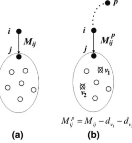
The information about the first node on each feasible path permits us to define new variables and a new coefficientMpijthat corresponds to an upper bound on the required capacity for archi;ji, when the directed path rooted at nodepincludes archi;ji. For some values ofpthis
bound may be smaller than the one given byMijand used in the previous model, leading to an improved linear programming relaxation.
Recall that the upper boundMijon the capacity required on archi;jiis defined by the sum of the demands of the nodes that can be served
through the arc. In this case, the concentrator that sends this traffic is not known in advance and theMijvalue is the sum of the node
de-mands reachable from archi;ji(Fig. 6a). To define the new coefficients, letp2Nandhi;ji 2Asuch that the directed path fromptojincludes archi;ji. The value of the maximum flow that can circulate on archi;jisent by nodepis equal to the sum of the demand of the nodes
reach-able from archi;jithat can be served by the concentrator located atp. This value will be denoted byMpij. If, by the elimination of some arcs,
some paths or some node to concentrator assignments, we can show that nodepcannot serve some of those nodes in any optimal solution, then theMpijvalue for some indexespmay become less than theMijcoefficient (Fig. 6b). For the auxiliary arch0;ji, we define as before the coefficientM0jas the total demand that can be served by the concentrator located atj.
The model uses binary variablesxp
ijindicating whether or not archi;ji 2Ais included in a directed path rooted at nodep(ifx p
ij¼1, nodes
iandjare assigned to the concentrator located at nodepÞ. These variables are defined for each pairðp;hi;jiÞonly if the directed path fromp
Table 1
Linear programming bound ofFA0formulation with the inclusion of different sets of valid inequalities.
Instance FA0 FA0+(8)+
(9)+(10)
FA0+(11) FA0+(11)+(12) FA0+ (11)+
(12)+ (13)
FA0+ (11)+ (12)+
(13)+ (14)+ (15)
FA0+ (11)+ (12)+ (13)+ (14)+
(15)+ (16)+ (17)
FA1 Opt.
tree10 1522.6 2041.1 2012.4 2130.7 2161.7 2169.2 2170.5 2170.5 2280
tree10_Fx2 1616.7 2303.7 2123.6 2301.1 2504.9 2520.5 2521.9 2527.1 2620
tree10_Bx2 1396.2 1693.2 1544.9 1562.2 1597.5 1658.3 1665.6 1704.6 1740
Fig. 5.(a) Concentrator at nodepprocess nodejdemand inT(b)h0;piis in the solution inD0and nodepprocess nodejdemand and all the demand of the nodes from the path
fromptoj.
tojtraverses archi;ji. In a similar way, we define nonnegative flow variablesypijindicating the amount of flow sent from the concentrator at
nodepthat circulates in archi;ji. For the auxiliary arcs, we define the binary variablesx0jindicating whether or not a concentrator is located
at nodejand the flow variablesy0jindicating the total demand served by that concentrator. To model the expansion of the links, we define
the binary variableszpijindicating whether or not archi;ji, belonging to the directed path rooted atp, is expanded and the nonnegative
vari-ablessp
ijdenoting the respective expanded amount of flow. Note that the new and the variables of theFAmodel are related as follows:
X
n
p¼1
xpij¼xij; X n
p¼1
ypij¼yij;
X
n
p¼1
zpij¼zijand
X
n
p¼1
spij¼sij: ð18Þ
The summation terms in these expressions can be simplified by noting that the index ‘‘p” is not considered wheneveriorjcannot be served by the concentrator located at nodep.
The formulation, denoted byNRFA, involving the new variables is as follows:
Minimize X
n
j¼1
Fjx0jþ
X
n
j¼1
cjy0jþ
X
hi;ji2A
X
n
p¼1
Gijzpijþ
X
hi;ji2A
X
n
p¼1
eijspij
subject to X
i:hi;ji2A0
X
n
p¼1
xp
ij¼1
8
j2N; ð19ÞX
i:hi;ji2A0
ypij
X
i:hj;ii2A
ypji¼dj; X i:hi;ji2A0
xpij
8
j2N8
p2N; ð20Þzpij6x p
ij
8
hi;ji 2A8
p2N; ð21Þ ypij6Bijxpijþs p
ij
8
hi;ji 2A8
p2N; ð22Þy0j6M0jx0j
8
j2N; ð23Þspij6 M p ijBij
zpij
8
hi;ji 2A8
p2N; ð24Þxpij2 f0;1g; y p
ijP0
8
hi;ji 2A0; p2N; zpij2 f0;1g; s pijP0
8
hi;ji 2A; p2N: ð25Þ We omit the description of the objective function and constraints in the new model since it can be taken from the description of the constraints in theFAmodel and the constraints(18)linking the two sets of variables. Note the new coefficientsMpijappearing in constraints (24). Recall that these coefficients may become smaller than the corresponding coefficient in theFAmodel when it is known that nodep(the corresponding concentrator) will not serve some nodes in the tree. Although the new model includes many more variables and con-straints than theFAmodel, the proposed pre-processing permits us to eliminate several directed paths and consequently eliminate many variables and constraints as well as reduce the value of theMp
ijcoefficient (in fact, it was the pre-processing leading to a reduction in theM p ij
coefficients that has motivated this model).
Result 4.1. The linear programming relaxation value of theNRFAformulation is greater or equal than the linear programming relaxation bound of theFA0formulation.
Proof. The result follows simply from the fact that by using(18), the constraints of theNRFAmodel imply the constraints of theFAmodel (note thatMp
ij6Mij; 8p2Nand all arcshi;jiÞ. The objective functions are the same after using(18). h
The computational results show that in general, theNRFAmodel already produces better lower bounds. However, the linear program-ming relaxation of the new model can be substantially improved by using the information attached to the new variables in order to derive new sets of inequalities:
xp
pk6x0p
8
hp;ki 2A; ð26Þ xpij6xp
pii
8
hi;ji 2A8
p2Nn fig; ð27Þwhere nodepiis the predecessor of nodeiin the directed path fromptoi. The constraints in the first set guarantee that if the archp;kiis
served by nodep(it means that the nodes associated to the arc are served by nodepÞa concentrator must be located atpand the constraints in the second set state, explicitly, the contiguity restriction for the archi;jiand the archpi;ii. The proof of the following result follows
imme-diately from these arguments.
Result 4.2. Inequalities(26) and (27)are valid for the LANEP.
Note that(26) and (27)guarantee thatxpij6x0p;8hi;ji 2A;8p2N, which, in turn, guarantee that a concentrator will be located at nodep
if this node serves archi;ji. The valid inequalities(26) and (27)are included in theNRFAformulation in order to improve its linear
program-ming relaxation. We denote byNRFA0the formulation obtained in this way.
4.2. Valid inequalities ‘‘adapted”from the FA model
In this subsection, we describe another interesting feature of the new formulation. Namely, we introduce valid inequalities that are similar to the ones introduced for theFAmodel and show that several of them are redundant in the linear programming relaxation of theNRFA0model.
4.2.1. 2-subtour elimination constraints
Using the relation between the new and old variables, the 2-subtour elimination constraints(8)can be rewritten as
X
n
p¼1
xp ijþ
X
n
p¼1
xp
ji61
8
ði;jÞ 2E; i;j–1: ð28ÞResult 4.3. Inequalities(28)are redundant to the linear programming relaxation ofNRFA0.
Proof.Let ði;jÞ 2E with i;j–1. Using constraints (19) for node j, the left-hand side of (28) can be rewritten as
Pn
p¼1x
p
ijþ
Pn
p¼1x
p
ji¼1x0jPk:hk;ji2A;k–i Pn
p¼1
p:k2Ppj xp
kjþx
j
jiþ
Pn
p¼1
p:j2Ppi;p–j
xp
ji, wherePpvdenotes the directed path from nodepto node
v.
Now, if we add constraints (27) for hj;ii and all p–j such that j is in the path from p to i, we obtain
Pn p¼1
p:j2Ppi;p–j
xpji6Pn
p¼1
p:j2Ppi xpp
jj¼
P
k:hk;ji2A;k–i
Pn
p¼1
p:k2Ppj
xpkj, and constraint (26) implies xjji6x0j. Combining these two inequalities with the
previous expression gives the desired inequality. h
4.2.2. Inequalities based on saturated nodes
The inequalities based on saturated nodes can be simply rewritten for the new model by using the relation between the new and old variables (for this case, we were unable to write disaggregated constraints as we did for many other inequalities): thus, for eachj2Ns, we
consider
X
k2TðjÞ x0kþ
X
n
p¼1
zpajjP1; ð29Þ
ðDðjÞ BajjÞ
X
k2TðjÞ x0k
0
@
1
Aþ
Xn
p¼1
spajjP DðjÞ Bajj: ð30Þ
4.2.3. Lower and upper bounding inequalities
We now analyse the lower bounding inequalities introduced before. These inequalities can be adapted to the new model by using the relation between the new and old variables or by considering their disaggregated versions. We consider the disaggregated versions to each of the inequalities presented before. We shall prove that several of the adapted inequalities are redundant to the linear programming relax-ation ofNRFA0.
Before presenting these inequalities and the redundancy of the results we make the following important observation. Observation: Let p;j2N: (i) If p–j, thenP
k:hk;ji2A0x
p
kj¼x
p
ij and
P k:hk;ji2A0y
p
kj¼y
p
ij, where hi;ji denotes the arc hpj;ji; (ii) If p¼j,
thenP k:hk;ji2A0x
p
kj¼x0jandPk:hk;ji2A0y
p
kj¼y0j(note that in (i) we are considering the directed path fromptojwhich has only one incident
arc injand (ii) represent the situation where nodejis served by a concentrator located at this node). The disaggregated version of constraints(11)–(13)are, respectively, constraints:
yp
ijPdjxpij
8
hi;ji 2A08
p2N; ð31Þ ypijPðdjþdkÞxpijþdkðxpjk1Þ
8
hi;ji 2A0; hj;ki 2Aðk–iÞ8
p2N; ð32Þyp
ijP djþ
X
k:hj;ki2A;k–i dk
!
xp ijþ
X
k:hj;ki2A;k–i
dkðxpjk1Þ
8
hi;ji 2A08
p2N: ð33ÞNote that we cannot include in(32) and (33)thexpkjterm (as we did for the aggregated versions inFA) because this variable is not de-fined in the new model. Note also that as observed before, these constraints are dede-fined only for specific triples (or m-tuples) of nodes.
Result 4.4. Inequalities(31)–(33)are redundant in the linear programming relaxation ofNRFA0.
Proof.We start by proving that constraints(31)are redundant to the linear programming relaxation ofNRFA0. Letp2Nandhi;ji 2A0. Assumep–j. Using the observation, the flow conservation constraints(20)becomeyp
ij¼djxpijþ P
k:hj;ki2A;k–iy p
jk. The nonnegativity of the
flow variables gives the desired inequalityypijPdjxpij. A similar argument is used whenp¼j, leading toy0jPdjx0j.
With respect to (32), note also that, for p–j and k–i, the expression ypij¼djxpijþ
P
v:hj;vi2A;v–iypjv can be rewritten as
ypij¼djxpijþy p jkþ
P
v:hj;vi2A;v–i;ky
p jv andy
p
ijPdjxpijþy p
jk. Using(31) in the previous expression (note thatjis in the path from nodepto nodekÞwe obtainyp
ijPdjxpijþdkxpjk. Sincedk xpij1
60, the previous inequality impliesypijPdjxpijþdkxpjkþdk xpij1
, which is the same
as the desired inequalityyp
ijPðdjþdkÞxpijþdk xpjk1
. A similar analysis holds whenp¼j.
The proof of(33)is similar and we omit it from the paper. h
The disaggregated version of the constraints(14) and (15)are, respectively, the constraints:
yp ij6 M
p ijM
p jk
xp ijþM
p jkx
p
jk
8
hi;ji 2A0; hj;ki 2Aðk–iÞ8
p2N; ð34Þ ypij6djxpijþ
X
k:hj;ki2A;k–i Mp
jkx p
jk
8
hi;ji 2A08
p2N: ð35ÞResult 4.5. Inequalities(34) and (35)are redundant in the linear programming relaxation ofNRFA0.
Proof. Note, first, that constraintsypij6Mpijxpij8hi;ji 2A08p2N(36) are guaranteed by constraints(22), (21) and (24), forhi;ji 2A, and by
(23) for the auxiliary arcs. We start by proving the redundancy of (35). Combining the flow conservation constraints
yp
ij¼djxpijþ P
k:hj;ki2A;k–iy p
jk with constraints (36) for the arcshj;ki 2A;k–i, we gety p
ij6djxpijþ P
k:hj;ki2A;k–iM p jkx
p
jk which is constraint(35)
forhi;ji 2A0andp2N.
With respect to constraints (34), let p2N;hi;ji 2A0 and hj;ki 2Aðk–iÞ. If p–j, the constraints (35) and the fact that
Mpij¼djþPv:hj;vi2A;v–iMpjvpermit us to rewrite constraint(35)forhi;ji 2A0andp2Nas followsy
p ij6 M
p ijM
p jk
P
v:hj;vi2A;v–k;iMpjvÞx
p ijþ
MpjkxpjkþP
v:hj;vi2A;v–k;iMpjvx
p
jv. By rearranging, we obtainy
p ij6 M
p ijM
p jk
xpijþMpjkxpjkþP
v:hj;vi2A;v–k;iMpjv x
p jvx
p ij
. Constraint(27)states
thatP
v:hj;vi2A;v–k;iMpjv x
p jvx
p ij
60 leading toypij6MpijMjkpxpijþMpjkxpjkwhich is(34)forhi;ji 2A0;hj;ki 2Aandp2N. Ifp¼jthe proof
is similar. h
The following result follows from the previous results.
Result 4.6. Inequalities(31)–(35)rewritten with the variables of theNRFAmodel by using(18)are redundant in the linear programming relaxation ofNRFA0.
Finally, the disaggregated version of the constraints(16) and (17)are, respectively, the constraints:
spij6 M p ijM
p jkBij
zpijþM p jkx
p
jk
8
hi;ji; hj;ki 2Aðk–iÞ8
p2N; ð37Þ spij6ðdjBijÞzpijþ
X
k:hj;ki2A;k–i Mp
jkx p
jk
8
hi;ji 2A8
p2N: ð38ÞOur computational results will show that these constraints are not redundant in the linear programming relaxation of theNRFA0model. We denote byNRFA1the formulationNRFA0augmented with(29), (30), (37), and (38). We present next the linear programming bounds
obtained withNRFAandNRFA0and the same formulation augmented with the several sets of inequalities in order to show that the inclu-sion of the different sets improve the cost of the linear programming solution to the instances presented inExample 3.1.
Example 4.1. Consider the local access network shown inFig. 4and the three instances used inExample 3.1.Table 2depicts the linear programming bounds obtained with theNRFAformulation, theNRFA0formulation and this formulation augmented with different sets of
the inequalities presented before, for instancestree10,tree10_Fx2andtree10_Bx2. The table description is omitted because is similar to Table 1.
The results show that the value of the linear programming relaxation of theNRFAformulation is quite improved by adding constraints (26) and (27), which are specially tailored to the new model.
5. Computational tests
5.1. Pre-processing
Pre-processing is an efficient way of reducing the size of the models. In some cases, pre-processing leads to an improvement on the value of the corresponding linear programming relaxation and to the reduction of the time used to obtain the solutions since eliminating a variable is equivalent to adding the inequality that sets to zero the value of the same variable. In this section, we show how to reduce some data coefficients and how to eliminate some variables from the models.
Table 2
Linear programming bound ofNRFAformulation.NRFA0formulation andNRFA0formulation augmented with the inclusion of different sets of valid inequalities.
Instance NRFA NRFA0 NRFA0 + (29)+(30) NRFA0 + (37)+(38) NRFA1 Opt.
tree10 2012.4 2220.2 2220.2 2221.3 2221.3 2280
tree10_Fx2 2123.6 2528.9 2528.9 2573.5 2573.5 2620
5.1.1. Coefficient reduction
Recall that theMijcoefficient represents the maximum flow that can circulate in an archi;jiand that theMpijcoefficient represents a
similar value when the arc is used in the directed path rooted at nodep. As referred, the initial values of these coefficients are set equal to the total demand of the nodes reachable through archi;ji. We present next several properties that permit us to define a better upper bound on the value of these coefficients.
By examining the costs of concentrators and links, it is possible to eliminate some node to concentrator assignments. Givenp;j2N,
Bal-akrishnan et al. (1995)show how to determine a lower bound to the cost of assign nodejto a concentrator located at nodep, denoted byLpj,
and an upper bound to the cost of installing a concentrator atj, denoted byUjj(seeBalakrishnan et al. (1995)for details).
Property 5.1. Letp;j2N. IfUjj<Lpj, nodepwill not serve nodejin any optimal solution.
Based on the elimination of node to concentrator assignments, it is possible to reduce or set equal to zero the values of the Mij and Mpij
coefficients. The next two properties show how this can be done.
Property 5.2.Lethi;ji 2Aandp2Nsuch that the pathPpjincludes archi;ji: (i) The total demand of the nodes that can be served by a con-centrator located at nodepthrough archi;jiis an upper bound to theMpijcoefficient; (ii) The value max
p2N M
p
ijis an upper bound to theMij
coefficient.
A particular case of the previous property is as follows:
Property 5.3. Lethi;ji 2A: (i) If any nodepcannot serve nodejthrough archi;ji, thenMij¼0 andMpij¼0, for allp2N; (ii) If some nodep cannot serve nodejthrough archi;ji, thenMpij¼0.
Note that in the context of the variables of theFAmodels, we can only set to zero theMijcoefficient ifanynodepcannot servejthrough
that arc.
Based on the fixed and variable costs of installing a concentrator at nodejand of expanding the archi;ji,Balakrishnan et al. (1995) deter-mine an upper bound to the valueMijby calculating the amount of flow from which it is cheaper to locate a concentrator at nodejrather than
expanding the archi;ji. This value is easily adapted for theMijpcoefficients. After using this property, some of the valuesMijandMpijmay
be-come smaller than the sum of the demands of the nodes reachable after archi;ji(or reachable afterhi;jiand in paths served by a concentrator inpin the case of theMpijcoefficients). In this case, the following property permits us to calculate these values in a different manner.
Property 5.4. Lethi;ji 2A0andhj;ki 2A, for allk2Nandk–i: (i) The valuedjþP
k:hj;ki2A;k–iMjkis an upper bound toMij; (ii) Letp2N. The valuedjþPk:hj;ki2A;k–iMpjkis an upper bound toM
p ij.
5.1.2. Variable elimination
We first show how coefficient reduction permit us to eliminate arcs and paths from the graphD0.
Property 5.5. Letj2Nandhi;ji 2A0: (i) IfMij<djorMpij<dj, for allp2N, the archi;jiwill not be used in any feasible solution; (ii) If Mpij<dj, for somep2N, the archi;jiwill not be used in the directed path rooted atpin any feasible solution (note that (i) and (ii) result from constraints(11) and (31), respectively).
We can generalize this property for the directed paths in the graph by considering the total demand of a sequence of nodes located ‘‘after” nodej. Recall thatPjkis the directed path from nodejto nodek.
Property 5.6.Lethi;ji 2A0;k2Nðk–jÞand let us assume that the pathPikincludes archi;ji. LetDjkbe the total demand from the pathPjk: (i) IfMij<DjkorMpij<Djk, for allp2N, then neither the pathPiknor any other path that includesPikcan be included in a feasible solution; (ii) IfMpij<Djk, for somep2N, then neither the pathPikrooted atpnor any path rooted atpthat includesPikcan be included in a feasible solution.
Note that if a pathPjkis eliminated from the graphD0than the assignment of nodekto a concentrator located injis also eliminated.
Finally, the next two properties show how to use the previous properties to eliminate variables from the models.
Property 5.7. Lethi;ji 2A: (i) If the archi;jiwill not be used in any feasible solution, then the variablesxij;yij;zijandsijcan be eliminated from theFAmodels as well as the variablesxpij;ypij;zpijandspij, for allp2N, can be eliminated from theNRFAmodels; (ii) If for somep2Nthe archi;jiwill not be used in the directed path rooted atpin any feasible solution, then the variablesxpij;ypij;zpijandspij, for the same indexesp,
can be eliminated from theNRFAmodels.
This property permit us to eliminate many variables from the models (this is more notorious in theNRFAmodel). The value of theMij
andMpijcoefficients (before or after reduction) also permits the elimination of the variables related to the expansion of the links.
Property 5.8. Lethi;ji 2A: (i) IfMij6Bij, then the archi;jiwill not be expanded in any feasible solution and the variableszijandsijcan be eliminated from theFAmodels as well as the variableszpijandspij, for allp2N, can be eliminated from theNRFAmodels; (ii) IfMpij6Bij, for somep2N, the variableszpijandspij, for the same indexesp, can be eliminated from theNRFAmodels.
Note also that the elimination of arcs/paths can also lead to a further reduction of severalMijandMpijcoefficients (if the corresponding
nodes are no longer reachable from an archi;ji, the maximum flow value in this arc can be reduced). Thus, the properties here suggested may and should be used more than once and iteratively until no further reduction or elimination is possible. The time used in the pre-pro-cessing is less than 1 s for instances with 100 and 200 nodes and, for instances with 500 nodes, the time is less or equal than to 3 s.
5.2. Computational results
We have compared three classes of flow-based formulations for the local access network expansion problem:FAandFDmodels (aggre-gated and disaggre(aggre-gated flow models, respectively) which were previously developed and the newNRFAmodel. Note, however, that theFA
model was significantly enhanced with the inclusion of the general lower and upper bounding inequalities. In this section, we present some computational results to assess their efficiency in solving instances of the problem and, in particular, we want to emphasize the advantages of developing the new model.
In order to evaluate and compare the linear programming relaxations of our models, we used instances with 100, 200 and 500 nodes. Some of these instances were already considered inCorte-Real and Gouveia (2007). Here we have included as well the 500-node instances and different scenarios for the smaller instances. The whole set includes two 100-node tree topologies, two 200-node tree topologies and two 500-node tree topologies, with two types of tree structure, which differ on the number of sons for each node. In the first case, this number is less or equal than 3 (trees 101, 201 and 501) and, in the second, is less or equal than 10 (trees 102, 202 and 502). For each tree, we have generated different set of parameters in order to represent three alternatives to expand the network, denoted byA;BandC, where Arepresents the situation that favours concentrator installation,Bfavours link expansion andCrepresents a more balanced alternative. Also, the number of links that need to be expanded, decreases fromAtoC. For each one of these 18 cases, we also varied some parameters in order to create different scenarios, considering several values for the node demands, links available capacities and costs. Thus, for each tree topology and each alternative (A;BorC), we have considered 14 more additional cases: we have divided the demand of each node by 5
and 2 and we have multiplied it by 2 (instances denoted by P/5, P/2 and P2, respectively); we have divided the available capacity of each arc by 2 and we have multiplied it by 2 and 5 (instances denoted by B/2, B2 and B5, respectively); we have divided the variable cost of the links by 2 and multiplied by 2, 5 and 20 (instances denoted by e/2, e2, e5 and e20, respectively) and we have divided the fixed cost of concentrators by 2 and multiplied it by 2, 5 and 20 (instances denoted by F/2, F2, F5 and F20, respectively). The results pre-sented in the following tables correspond to average values obtained with three instances, the three of them generated with the same char-acteristics. All the tests were run in an Intel Core 2 Duo, 2.00 GHz, personal computer with 2 GB of RAM, and the CPLEX package, version 10.2, has been used to obtain the linear programming bounds and the integer optimal solutions.
Before presenting and comparing in detail the results for the three classes of models, we first introduceTable 3in order to illustrate the effect of the pre-processing. This table shows the gaps for the instances with 100 nodes given by the optimal linear programming bound for formulationsFA0;FA1;NRFA0andNRFA1described before, with and without the pprocessing, and the corresponding CPU times (the
re-sults correspond to the average of the three alternatives). The first two columns specify the problem instances. The next eight columns present the gaps given by the value [(OPTLB)/OPT] * 100 (OPT is the value of the integer optimal solution and LB is the value of the low-er-bound given by the optimal linear programming solution of the model indicated at the top of the column). Next to this value we present two other values in parentheses: the first one is the CPU time needed to solve the linear programming relaxation and the second one is the CPU time needed to obtain the optimal value (time is given in seconds).
The results strongly indicate that pre-processing reduces significantly the gaps, in particular for theFA0formulation: the maximum reduction obtained is of 10.89% forFA0, 0.87% forFA1, 1.20% forNRFA0and 1.22% forNRFA1. Note, also, that the pre-processing has a great impact in the CPU times of theNRFAmodel because it eliminates many paths, leading to a substantial number of variables that were elim-inated from the model. This in turn, leads to a greater reduction in theMp
ijcoefficients. As stated before, it was this pre-processing leading to
a reduction in theMp
ijcoefficients that has motivated the idea for creating the new model.
In order to compare the models,Tables 4–6depict the gaps given by the optimal linear programming bound of the formulations
FA0;FA1;FD0;FD1,NRFA0andNRFA1, obtained with the pre-processing described. Each table corresponds to instances with the same number
of nodes and the two structures used. Each column is easily identified by the corresponding name at its top. We present, in the same way as before, the gap value and, in parentheses, the corresponding CPU times. The designationindicates that we were not able to solve the
inte-ger model within the time limit of 2 h.
The results indicate that theNRFAmodels produce, in general, the best linear programming bounds and that theFAmodels produce, as expected, the worst. However, we note that for the alternativesAandBthe three classes of models produce, in general, small gaps for all the instances giving some practical confirmation that the previous transformation of the LANEP into a CMSTP with additional constraints was worth developing (the exceptions are the cases with costs variation opposite to the network expansion type and whose necessity of expansion is reduced). We can also see that the three classes of models permit, in general, to obtain very quickly the optimal solutions to all instances with 100 and 200 nodes and to the instances with 500 nodes for alternativesAandB. With respect to the 500 nodes instances and for alternativeC, the models required in general more time. We identify cases whereFAmodels use less time than the others as well as the
NRFAmodels. Note that, in some problem instances, theNRFA1formulation produced the optimal solution in seconds while theFA1andFD1
Table 3
Average results for instances with 100 nodes, with and without pre-processing, forFAandNRFAmodels.
Instance FA0 FA1 NRFA0 NRFA1
without PP with PP without PP with PP without PP with PP without PP with PP
Results for instances with 100 nodes with pre-processing. for structures 101 and 102.
Instance FA1 FA1 FD1 FD1 NRFA1 NRFA1 Instance FA1 FA1 FD1 FD1 NRFA1 NRFA1
101A P/5 2.09 (0 + 0) 1.02 (0 + 0) 0.78(0 + 0) 0.71(0 + 0) 0.75 (0 + 0) 0.69(0 + 0) 102A P/5 3.58(0 + 0) 1.50(0 + 1) 1.08(0 + 1) 1.02 (0 + 2) 1.08(0 + 1) 1.02(0 + 1) P/2 0.39 (0 + 0) 0.17 (0 + 0) 0.20(0 + 0) 0.15(0 + 0) 0.20 (0 + 0) 0.14 (0 + 0) P/2 0.78(0 + 0) 0.38(0 + 0) 0.32 (0 + 0) 0.32(0 + 0) 0.32(0 + 0) 0.32 (0 + 0) P 0.02 (0 + 0) 0.01 (0 + 0) 0.01 (0 + 0) 0.01(0 + 0) 0.01 (0 + 0) 0.01 (0 + 0) P 0.17 (0 + 0) 0.06(0 + 0) 0.06 (0 + 0) 0.03(0 + 0) 0.06(0 + 0) 0.03 (0 + 0) P2 0.00 (0 + 0) 0.00 (0 + 0) 0.00(0 + 0) 0.00 (0 + 0) 0.00 (0 + 0) 0.00(0 + 0) P2 0.03(0 + 0) 0.01(0 + 0) 0.01(0 + 0) 0.01 (0 + 0) 0.01 (0 + 0) 0.01(0 + 0) F/2 0.02 (0 + 0) 0.01 (0 + 0) 0.01 (0 + 0) 0.01(0 + 0) 0.01 (0 + 0) 0.01 (0 + 0) F/2 0.17 (0 + 0) 0.06(0 + 0) 0.06 (0 + 0) 0.03(0 + 0) 0.06(0 + 0) 0.03 (0 + 0) F2 0.09 (0 + 0) 0.02 (0 + 0) 0.03(0 + 0) 0.02 (0 + 0) 0.03 (0 + 0) 0.02(0 + 0) F2 0.23(0 + 0) 0.06(0 + 0) 0.06 (0 + 0) 0.03(0 + 0) 0.06(0 + 0) 0.03 (0 + 0) F5 0.36 (0 + 0) 0.03 (0 + 0) 0.04(0 + 0) 0.03 (0 + 0) 0.04 (0 + 0) 0.03(0 + 0) F5 0.55(0 + 0) 0.11 (0 + 0) 0.14(0 + 0) 0.10 (0 + 0) 0.14 (0 + 0) 0.10(0 + 0) F20 2.40 (0 + 0) 0.14 (0 + 0) 0.14 (0 + 0) 0.12(0 + 0) 0.14 (0 + 0) 0.11 (0 + 0) F20 3.53(0 + 0) 0.25(0 + 0) 0.04 (0 + 0) 0.03(0 + 0) 0.04(0 + 0) 0.03 (0 + 0) e/2 0.14(0 + 0) 0.07 (0 + 0) 0.08(0 + 0) 0.07 (0 + 0) 0.08 (0 + 0) 0.06(0 + 0) e/2 0.19 (0 + 0) 0.02(0 + 0) 0.03 (0 + 0) 0.02(0 + 0) 0.03(0 + 0) 0.02 (0 + 0) e2 0.02 (0 + 0) 0.01 (0 + 0) 0.01 (0 + 0) 0.01(0 + 0) 0.01 (0 + 0) 0.01 (0 + 0) e2 0.10 (0 + 0) 0.05(0 + 0) 0.03 (0 + 0) 0.03(0 + 0) 0.03(0 + 0) 0.03 (0 + 0) e5 0.07 (0 + 0) 0.01 (0 + 0) 0.01 (0 + 0) 0.01(0 + 0) 0.01 (0 + 0) 0.01 (0 + 0) e5 0.08(0 + 0) 0.04(0 + 0) 0.02 (0 + 0) 0.02(0 + 0) 0.02(0 + 0) 0.02 (0 + 0) e20 0.01(0 + 0) 0.00 (0 + 0) 0.00(0 + 0) 0.00 (0 + 0) 0.00 (0 + 0) 0.00(0 + 0) e20 0.10 (0 + 0) 0.08(0 + 0) 0.09 (0 + 0) 0.08(0 + 0) 0.08(0 + 0) 0.09 (0 + 0) B/2 0.01(0 + 0) 0.00 (0 + 0) 0.00(0 + 0) 0.00 (0 + 0) 0.00 (0 + 0) 0.00(0 + 0) B/2 0.06(0 + 0) 0.01(0 + 0) 0.02 (0 + 0) 0.01 (0 + 0) 0.02(0 + 0) 0.01(0 + 0) B2 0.26 (0 + 0) 0.13 (0 + 0) 0.13 (0 + 0) 0.11 (0 + 0) 0.13 (0 + 0) 0.11 (0 + 0) B2 0.56(0 + 0) 0.36(0 + 0) 0.28 (0 + 0) 0.28(0 + 0) 0.28(0 + 0) 0.28 (0 + 0) B5 1.06(0 + 0) 0.71 (0 + 0) 0.43(0 + 0) 0.41(0 + 0) 0.40 (0 + 0) 0.38(0 + 0) B5 1.71(0 + 0) 1.12 (0 + 0) 0.81(0 + 1) 0.77(0 + 1) 0.81 (0 + 0) 0.77 (0 + 1)
101B P/5 1.26(0 + 0) 1.03 (0 + 0) 0.96(0 + 1) 0.90 (0 + 1) 0.90 (0 + 2) 0.88(0 + 2) 102B P/5 0.00(0 + 0) 0.00(0 + 0) 0.00 (0 + 0) 0.00(0 + 0) 0.00(0 + 0) 0.00 (0 + 0) P/2 2.47 (0 + 0) 2.01 (0 + 0) 1.62 (0 + 1) 1.61 (0 + 1) 1.60 (0 + 2) 1.59 (0 + 3) P/2 0.00(0 + 0) 0.00(0 + 0) 0.00 (0 + 0) 0.00(0 + 0) 0.00(0 + 0) 0.00 (0 + 0) P 1.35(0 + 0) 1.10(0 + 0) 0.78(0 + 0) 0.77 (0 + 1) 0.78 (0 + 2) 0.77(0 + 3) P 0.03(0 + 0) 0.00(0 + 0) 0.03(0 + 0) 0.00(0 + 0) 0.03(0 + 0) 0.00 (0 + 0) P2 0.40 (0 + 0) 0.24 (0 + 0) 0.15 (0 + 0) 0.15(0 + 0) 0.15 (0 + 0) 0.15 (0 + 1) P2 0.00(0 + 0) 0.00(0 + 0) 0.00 (0 + 0) 0.00(0 + 0) 0.00(0 + 0) 0.00 (0 + 0) F/2 1.35(0 + 0) 1.10(0 + 0) 0.78(0 + 1) 0.77 (0 + 0) 0.78 (0 + 2) 0.77(0 + 3) F/2 0.03(0 + 0) 0.00(0 + 0) 0.03 (0 + 0) 0.00(0 + 0) 0.03(0 + 0) 0.00 (0 + 0) F2 1.36(0 + 0) 1.10(0 + 0) 0.79(0 + 1) 0.77 (0 + 1) 0.79 (0 + 3) 0.77(0 + 3) F2 0.03(0 + 0) 0.00(0 + 0) 0.02 (0 + 0) 0.00(0 + 0) 0.02(0 + 0) 0.00 (0 + 0) F5 1.37(0 + 0) 1.10(0 + 0) 0.79(0 + 1) 0.77 (0 + 1) 0.79 (0 + 2) 0.77(0 + 3) F5 0.04(0 + 0) 0.00(0 + 0) 0.02 (0 + 0) 0.00(0 + 0) 0.02(0 + 0) 0.00 (0 + 0) F20 1.45(0 + 0) 1.10(0 + 0) 0.79(0 + 1) 0.77 (0 + 1) 0.79 (0 + 2) 0.77(0 + 4) F20 0.05(0 + 0) 0.00(0 + 0) 0.02 (0 + 0) 0.00(0 + 0) 0.02(0 + 0) 0.00 (0 + 0) e/2 0.12(0 + 0) 0.02 (0 + 0) 0.02(0 + 0) 0.01(0 + 0) 0.02 (0 + 0) 0.01 (0 + 0) e/2 0.00(0 + 0) 0.00(0 + 0) 0.00 (0 + 0) 0.00(0 + 0) 0.00(0 + 0) 0.00 (0 + 0) e2 1.33(0 + 0) 1.15(0 + 0) 0.78(0 + 0) 0.78 (0 + 0) 0.77 (0 + 1) 0.77(0 + 1) e2 0.08(0 + 0) 0.11 (0 + 0) 0.00 (0 + 0) 0.00(0 + 0) 0.00(0 + 0) 0.00 (0 + 1) e5 3.28 (0 + 0) 2.73 (0 + 0) 2.23(0 + 1) 2.20 (0 + 0) 2.15 (0 + 0) 2.13 (0 + 1) e5 3.89(0 + 0) 2.38(0 + 0) 1.04(0 + 1) 1.04 (0 + 1) 1.04 (0 + 2) 1.04(0 + 2) e20 4.73 (0 + 0) 3.79 (0 + 0) 2.71 (0 + 0) 2.71(0 + 0) 2.59 (0 + 0) 2.59(0 + 0) e20 8.87(0 + 0) 4.87(0 + 0) 3.44 (0 + 2) 3.37(0 + 2) 3.43(0 + 4) 3.36 (0 + 5) B/2 0.41(0 + 0) 0.24 (0 + 0) 0.15 (0 + 0) 0.15(0 + 0) 0.15 (0 + 0) 0.15 (0 + 0) B/2 0.00(0 + 0) 0.00(0 + 0) 0.00 (0 + 0) 0.00(0 + 0) 0.00(0 + 0) 0.00 (0 + 0) B2 2.46 (0 + 0) 2.01 (0 + 0) 1.62 (0 + 1) 1.61 (0 + 1) 1.60 (0 + 2) 1.59 (0 + 4) B2 0.00(0 + 0) 0.00(0 + 0) 0.00 (0 + 0) 0.00(0 + 0) 0.00(0 + 0) 0.00 (0 + 0) B5 1.20(0 + 0) 1.02 (0 + 0) 0.94(0 + 1) 0.89 (0 + 1) 0.88 (0 + 1) 0.87(0 + 1) B5 0.00(0 + 0) 0.00(0 + 0) 0.00 (0 + 0) 0.00(0 + 0) 0.00(0 + 0) 0.00 (0 + 0)
101C P/5 32.24(0 + 0) 15.87 (0 + 1) 6.74(0 + 5) 5.50 (0 + 4) 6.45 (0 + 7) 5.19 (1 + 5) 102C P/5 35.21 (0 + 0) 18.90 (0 + 1) 15.37 (1 + 3) 14.10(1 + 4) 15.37 (5 + 13) 14.10 (4 + 15) P/2 22.66(0 + 0) 10.81(0 + 1) 8.85(0 + 1) 8.08 (0 + 2) 8.45 (0 + 2) 7.85(0 + 2) P/2 29.71 (0 + 0) 12.85 (0 + 1) 12.26(0 + 5) 11.68(0 + 4) 12.21 (2 + 7) 11.69 (3 + 11) P 15.04(0 + 0) 8.36 (0 + 1) 6.67(0 + 1) 5.95 (0 + 1) 5.88 (0 + 0) 5.40(0 + 0) P 20.09(0 + 0) 7.15(0 + 0) 6.09 (0 + 4) 5.76(0 + 3) 6.06(0 + 6) 5.75 (1 + 5) P2 7.83 (0 + 0) 4.71 (0 + 0) 2.60(0 + 0) 2.58(0 + 0) 2.51 (0 + 0) 2.48(0 + 0) P2 12.35 (0 + 0) 4.18(0 + 0) 1.88(0 + 1) 1.94 (0 + 1) 1.87 (0 + 2) 1.84(0 + 2) F2 12.26(0 + 0) 7.92 (0 + 0) 6.60(0 + 1) 6.00 (0 + 0) 5.76 (0 + 0) 5.39(0 + 0) F2 15.30 (0 + 0) 7.38(0 + 0) 6.41(0 + 3) 6.12 (0 + 2) 6.36(0 + 6) 6.07 (1 + 7) F2 20.62(0 + 0) 9.11(0 + 1) 6.99(0 + 1) 6.36 (0 + 1) 6.36 (0 + 0) 5.84(0 + 1) F2 26.82(0 + 0) 6.96(0 + 0) 5.26 (0 + 4) 4.83(0 + 5) 5.25 (1 + 4) 4.93 (2 + 5) F5 30.66 (0 + 1) 10.68 (0 + 1) 5.80(0 + 3) 5.58 (0 + 2) 4.96 (0 + 1) 4.82(0 + 2) F5 34.79(0 + 0) 5.50(0 + 0) 2.76 (1 + 3) 2.22(1 + 2) 2.74(5 + 5) 2.22 (8 + 5) F20 47.23(0 + 2) 16.48(0 + 3) 4.82(1 + 6) 4.47 (1 + 6) 4.68 (1 + 7) 4.43(1 + 14) F20 46.63(0 + 0) 8.87(0 + 1) 2.79 (2 + 3) 2.63(2 + 2) 2.28(8 + 4) 2.16(16 + 36) e/2 15.78(0 + 0) 7.70 (0 + 1) 6.32(0 + 1) 5.87 (0 + 2) 5.82 (0 + 0) 5.46(0 + 1) e/2 18.38 (0 + 0) 6.16(0 + 0) 4.77 (0 + 3) 4.24(0 + 2) 4.67 (1 + 5) 4.15(1 + 9) e2 13.04(0 + 0) 7.89 (0 + 0) 5.45(0 + 0) 4.48 (0 + 0) 4.79 (0 + 0) 3.90(0 + 0) e2 17.84 (0 + 0) 7.65(0 + 1) 6.94 (0 + 3) 6.71 (0 + 4) 6.84(0 + 5) 6.62 (0 + 7) e5 12.16 (0 + 0) 7.89 (0 + 0) 5.16 (0 + 0) 4.00 (0 + 0) 4.55 (0 + 0) 3.41 (0 + 0) e5 16.75 (0 + 0) 8.30(0 + 1) 7.34 (0 + 4) 7.28(0 + 4) 7.24(0 + 5) 7.18(0 + 7) e20 10.34(0 + 0) 5.75 (0 + 0) 3.86(0 + 0) 2.81(0 + 0) 3.38 (0 + 0) 2.33(0 + 0) e20 15.20 (0 + 1) 8.81(0 + 1) 7.78 (0 + 6) 7.74(0 + 7) 7.62(0 + 6) 7.58 (0 + 6) B/2 10.38(0 + 0) 5.18 (0 + 0) 3.18 (0 + 0) 3.15(0 + 0) 2.92 (0 + 0) 2.85(0 + 0) B/2 16.18(0 + 0) 4.32(0 + 0) 1.85(0 + 2) 1.84 (0 + 1) 1.94 (0 + 2) 1.83(0 + 3) B2 17.34(0 + 0) 9.42 (0 + 0) 7.97(0 + 1) 7.09 (0 + 1) 7.56 (0 + 1) 6.89(0 + 1) B2 25.46(0 + 0) 13.87 (0 + 1) 12.48(0 + 5) 12.06 (0 + 5) 12.33 (1 + 7) 12.06(1 + 10) B5 16.82(0 + 0) 11.10 (0 + 1) 7.26(0 + 1) 6.90 (0 + 1) 7.26 (0 + 2) 6.88(0 + 3) B5 24.79(0 + 0) 17.31 (0 + 0) 13.57(0 + 3) 12.64 (0 + 3) 13.57 (1 + 10) 12.64(2 + 6)
M.
Corte-Real,
L.
Gouveia
/European
Journal
of
Operational
Research
204
(2010)
20–34
Table 5
Results for instances with 200 nodes with pre-processing. for structures 201 and 202.
Instance FA1 FA1 FD1 FD1 MRFA1 NRFA1 Instance FA1 FA1 FD1 FD1 NRFA1 NRFA1
201A P/5 2.32 (0 + 11) 1.26(0 + 6) 0.87(0 + 2) 0.74 (0 + 2) 0.84 (0 + 0) 0.68 (0 + 0) 202A P/5 2.88 (0 + 17) 1.21 (0 + 8) 0.84(0 + 78) 0.81(0 + 83) 0.82 (0 + 3) 0.79(0 + 5) P/2 0.57 (0 + 0) 0.20(0 + 0) 0.23(0 + 0) 0.17 (0 + 0) 0.22 (0 + 0) 0.17(0 + 0) P/2 0.82 (0 + 0) 0.30(0 + 0) 0.29(0 + 0) 0.25 (0 + 0) 0.28 (0 + 0) 0.24(0 + 0) P 0.08 (0 + 0) 0.03(0 + 0) 0.03(0 + 0) 0.03 (0 + 0) 0.03 (0 + 0) 0.03 (0 + 0) P 0.16(0 + 0) 0.06(0 + 0) 0.05(0 + 0) 0.05 (0 + 0) 0.05 (0 + 0) 0.05(0 + 0) P2 0.01(0 + 0) 0.01(0 + 0) 0.01 (0 + 0) 0.01(0 + 0) 0.01(0 + 0) 0.01(0 + 0) P2 0.04 (0 + 0) 0.01 (0 + 0) 0.01 (0 + 0) 0.01(0 + 0) 0.01(0 + 0) 0.01(0 + 0) F/2 0.07 (0 + 0) 0.03(0 + 0) 0.03(0 + 0) 0.03 (0 + 0) 0.03 (0 + 0) 0.03 (0 + 0) F/2 0.13(0 + 0) 0.05(0 + 0) 0.05(0 + 0) 0.05 (0 + 0) 0.05 (0 + 0) 0.05(0 + 0) F2 0.12(0 + 0) 0.03(0 + 0) 0.03(0 + 0) 0.03 (0 + 0) 0.03 (0 + 0) 0.03 (0 + 0) F2 0.28 (0 + 0) 0.06(0 + 0) 0.05(0 + 0) 0.05 (0 + 0) 0.05 (0 + 0) 0.05(0 + 0) F5 0.36 (0 + 0) 0.07(0 + 0) 0.04(0 + 0) 0.03 (0 + 0) 0.03 (0 + 0) 0.03 (0 + 0) F5 0.60 (0 + 0) 0.09(0 + 0) 0.06(0 + 0) 0.06 (0 + 0) 0.06 (0 + 0) 0.05(0 + 0) F20 3.28 (0 + 0) 0.26(0 + 0) 0.18 (0 + 0) 0.15 (0 + 0) 0.18(0 + 0) 0.12(0 + 0) F20 3.07 (0 + 0) 0.23(0 + 0) 0.06(0 + 0) 0.05 (0 + 0) 0.06 (0 + 0) 0.04(0 + 0) e/2 0.19(0 + 0) 0.07(0 + 0) 0.07(0 + 0) 0.06 (0 + 0) 0.07 (0 + 0) 0.06 (0 + 0) e/2 0.21(0 + 0) 0.04(0 + 0) 0.06(0 + 0) 0.04 (0 + 0) 0.06 (0 + 0) 0.04(0 + 0) e2 0.04 (0 + 0) 0.01(0 + 0) 0.00(0 + 0) 0.00 (0 + 0) 0.00 (0 + 0) 0.00 (0 + 0) e2 0.13(0 + 0) 0.07(0.0) 0.06(0 + 0) 0.06 (0 + 0) 0.06 (0 + 0) 0.06(0 + 0) e5 0.02 (0 + 0) 0.00(0 + 0) 0.00(0 + 0) 0.00 (0 + 0) 0.00 (0 + 0) 0.00 (0 + 0) e5 0.06 (0 + 0) 0.04(0 + 0) 0.04(0 + 0) 0.04 (0 + 0) 0.04 (0 + 0) 0.04(0 + 0) e20 0.02 (0 + 0) 0.00(0 + 0) 0.00(0 + 0) 0.00 (0 + 0) 0.00 (0 + 0) 0.00 (0 + 0) e20 0.03 (0 + 0) 0.02(0 + 0) 0.02(0 + 0) 0.02 (0 + 0) 0.02 (0 + 0) 0.02(0 + 0) B/2 0.01(0 + 0) 0.01(0 + 0) 0.01 (0 + 0) 0.01(0 + 0) 0.01(0 + 0) 0.01(0 + 0) B/2 0.05 (0 + 0) 0.02(0 + 0) 0.02(0 + 0) 0.02 (0 + 0) 0.02 (0 + 0) 0.01(0 + 0) B2 0.36 (0 + 0) 0.15(0 + 0) 0.14 (0 + 0) 0.13 (0 + 0) 0.13(0 + 0) 0.12(0 + 0) B2 0.64 (0 + 0) 0.24(0 + 0) 0.22(0 + 0) 0.20 (0 + 0) 0.22 (0 + 0) 0.20(0 + 0) B5 1.13(0 + 2) 0.72(0 + 1) 0.52(0 + 1) 0.46 (0 + 1) 0.51(0 + 0) 0.45 (0 + 0) B5 1.32(0 + 3) 0.78(0 + 4) 0.51 (0 + 17) 0.48 (0 + 27) 0.50 (0 + 3) 0.48(0 + 3)
201B P/5 3.19(0 + 0) 3.07(0 + 1) 2.41 (0 + 5) 2.40 (0 + 6) 2.39 (1 + 14) 2.38 (1 + 10) 202B P/5 0.20 (0 + 0) 0.18 (0 + 0) 0.18 (0 + 1) 0.18(0 + 1) 0.19(1 + 0) 0.18(1 + 1) P/2 0.83 (0 + 0) 0.67(0 + 1) 0.54(0 + 2) 0.46 (0 + 2) 0.54 (0 + 2) 0.46 (0 + 7) P/2 0.06 (0 + 0) 0.05(0 + 0) 0.05(0 + 1) 0.05 (0 + 1) 0.05 (0 + 1) 0.05(0 + 1) P 0.40 (0 + 0) 0.32(0 + 0) 0.15 (0 + 1) 0.15 (0 + 1) 0.15(0 + 3) 0.15(0 + 3) P 0.33 (0 + 0) 0.02(0 + 0) 0.01 (0 + 1) 0.00 (0 + 1) 0.01(0 + 1) 0.00(0 + 1) P2 0.19(0 + 0) 0.07(0 + 0) 0.02(0 + 0) 0.01(0 + 0) 0.02 (0 + 0) 0.01(0 + 1) P2 0.27 (0 + 0) 0.10 (0 + 0) 0.00(0 + 1) 0.00 (0 + 1) 0.00 (0 + 1) 0.00(0 + 1) F/2 0.40 (0 + 0) 0.32(0 + 0) 0.16 (0 + 1) 0.15 (0 + 1) 0.16(0 + 4) 0.15(0 + 2) F/2 0.32 (0 + 0) 0.02(0 + 0) 0.01 (0 + 1) 0.00 (0 + 1) 0.01(0 + 1) 0.00(0 + 1) F2 0.40 (0 + 0) 0.32(0 + 0) 0.15 (0 + 1) 0.15 (0 + 1) 0.15(0 + 4) 0.15(0 + 3) F2 0.34 (0 + 0) 0.02(0 + 0) 0.01 (0 + 1) 0.00 (0 + 1) 0.01(0 + 1) 0.00(0 + 1) F5 0.41(0 + 0) 0.32(0 + 0) 0.15 (0 + 1) 0.14 (0 + 1) 0.15(0 + 3) 0.14(0 + 3) F5 0.35 (0 + 0) 0.02(0 + 0) 0.01 (0 + 1) 0.00 (0 + 1) 0.01(0 + 1) 0.00(0 + 1) F20 0.47 (0 + 0) 0.42(0 + 0) 0.15 (0 + 1) 0.14 (0 + 1) 0.15(0 + 2) 0.14(0 + 3) F20 0.44 (0 + 0) 0.02(0 + 0) 0.00(0 + 1) 0.00 (0 + 1) 0.00 (0 + 1) 0.00(1 + 0) e/2 0.22 (0 + 0) 0.18(0 + 0) 0.14 (0 + 1) 0.13 (0 + 1) 0.14(0 + 2) 0.13(0 + 2) e/2 0.01(0 + 0) 0.00(0 + 0) 0.01 (0 + 1) 0.00 (0 + 1) 0.01(0 + 1) 0.00(0 + 1) e2 1.15(0 + 0) 0.93(0 + 1) 0.67(0 + 2) 0.62 (0 + 2) 0.62 (0 + 2) 0.58 (0 + 5) e2 0.85 (0 + 0) 0.35(0 + 0) 0.08(0 + 1) 0.05 (0 + 1) 0.08 (1 + 0) 0.05(1 + 1) e5 2.49 (0 + 0) 2.11 (0 + 1) 1.44 (0 + 1) 1.42 (0 + 2) 1.33(0 + 1) 1.31 (0 + 2) e5 2.58 (0 + 0) 1.92 (0 + 1) 0.64(1 + 3) 0.56 (1 + 3) 0.64 (1 + 9) 0.56 (1 + 11) e20 4.38 (0 + 1) 3.52(0 + 1) 3.19 (0 + 2) 3.13 (0 + 2) 2.99 (0 + 0) 2.84 (0 + 1) e20 3.68 (0 + 1) 2.47(0 + 1) 1.78 (1 + 8) 1.66 (1 + 8) 1.76(1 + 14) 1.65 (1 + 12) B/2 0.19(0 + 0) 0.07(0 + 0) 0.02(0 + 0) 0.01(0 + 0) 0.02 (0 + 0) 0.01(0 + 1) B/2 0.28 (0 + 0) 0.10 (0 + 0) 0.00(0 + 1) 0.00 (0 + 1) 0.00 (0 + 1) 0.00(0 + 1) B2 0.82 (0 + 0) 0.67(0 + 1) 0.54(0 + 2) 0.46 (0 + 2) 0.54 (0 + 2) 0.46 (1 + 4) B2 0.05 (0 + 0) 0.05(0 + 0) 0.05(0 + 1) 0.05 (0 + 1) 0.05 (0 + 1) 0.05(1 + 0) B5 3.14(0 + 0) 3.06(0 + 1) 2.40(0 + 5) 2.39 (0 + 6) 2.38 (0 + 11) 2.38 (1 + 11) B5 0.19(0 + 0) 0.18 (0 + 0) 0.18 (0 + 1) 0.18(0 + 1) 0.18(1 + 0) 0.18(1 + 1)
201C P/5 30.46 (0 + 3) 17.56 (0 + 10) 15.54 (3 + 125) 13.42(3 + 138) 14.80(9 + 116) 12.95(10 + 290) 202C P/5 28.25(0 + 1) 7.83(0 + 1) 7.22(4 + 23) 6.36 (4 + 20) 7.20 (24 + 60) 6.36(25 + 85) P/2 19.89(0 + 5) 11.92 (0 + 9) 8.55(1 + 50) 7.76 (1 + 50) 7.95 (1 + 28) 7.19(1 + 24) P/2 19.51 (0 + 0) 6.62(0 + 1) 5.55(2 + 21) 5.40 (3 + 14) 5.54 (6 + 25) 5.38(11 + 55) P 11.76 (0 + 3) 6.24(0 + 3) 4.92(0 + 16) 4.37 (0 + 12) 4.54 (0 + 3) 4.08 (0 + 3) P 13.90(0 + 0) 4.25(0 + 1) 3.49 (1 + 12) 3.43 (1 + 13) 3.48 (2 + 15) 3.43(2 + 18) P2 8.04 (0 + 1) 4.80(0 + 1) 4.03(0 + 1) 3.71 (0 + 1) 3.94 (0 + 0) 3.61(0 + 0) P2 8.26 (0 + 0) 2.72(0 + 1) 1.64 (0 + 2) 1.52(0 + 2) 1.61 (0 + 1) 1.48(0 + 4) F/2 9.05 (0 + 2) 5.77(0 + 3) 4.17 (0 + 6) 3.90 (0 + 7) 3.95 (0 + 2) 3.68 (0 + 2) F/2 10.60(0 + 1) 4.14 (0 + 1) 3.58 (1 + 14) 3.50 (1 + 17) 3.57 (1 + 11) 3.49(2 + 16) F2 16.22(0 + 3) 6.90(0 + 6) 4.80(0 + 18) 4.24 (0 + 16) 4.45 (0 + 4) 3.87 (0 + 5) F2 18.98(0 + 1) 4.61 (0 + 1) 3.16 (1 + 12) 3.05 (1 + 14) 3.14(3 + 20) 3.04(5 + 42) F5 24.54 (0 + 7) 8.19(0 + 7) 4.60(1 + 26) 3.84 (0 + 31) 4.17(0 + 8) 3.38 (1 + 9) F5 27.50(0 + 1) 6.08(0 + 2) 3.56(3 + 25) 3.38 (2 + 23) 3.56 (11 + 41) 3.37(17 + 98) F20 39.94 (0 + 15) 12.68 (0 + 45) 5.01 (3 + 213) 4.42 (3 + 148) 4.49 (2 + 53) 4.06 (4 + 88) F20 35.04(0 + 1) 6.98(0 + 2) 1.68 (7 + 8) 1.64 (7 + 11) 1.68(25 + 43) 1.63(33 + 51) e/2 12.12 (0 + 2) 5.28(0 + 3) 3.97(0 + 11) 3.43 (0 + 11) 3.78 (0 + 4) 3.36 (0 + 12) e/2 13.31 (0 + 0) 3.68(0 + 1) 2.64(1 + 8) 2.48 (1 + 8) 2.64 (3 + 14) 2.48(5 + 21) e2 11.35 (0 + 4) 6.33(0 + 4) 4.61 (0 + 8) 4.26 (0 + 8) 4.46 (0 + 4) 4.10(0 + 3) e2 13.28(0 + 2) 4.97(0 + 2) 4.31 (1 + 70) 4.17(1 + 176) 4.31(1 + 12) 4.16 (1 + 15) e5 11.15 (0 + 6) 7.49(0 + 9) 4.70(0 + 7) 4.61(0 + 6) 4.61(0 + 1) 4.53 (0 + 2) e5 12.10 (0 + 1) 5.46(0 + 2) 5.15 (1 + 60) 4.84 (1 + 56) 5.15(1 + 12) 4.84 (1 + 11) e20 10.88(0 + 3) 7.68(0 + 4) 4.79(0 + 6) 4.55 (0 + 6) 4.71(0 + 1) 4.48 (0 + 2) e20 11.02 (0 + 1) 5.62(0 + 1) 5.58 (1 + 18) 5.24 (1 + 18) 5.58 (1 + 8) 5.24(1 + 13) B/2 11.16 (0 + 4) 5.66(0 + 2) 4.58(0 + 2) 4.27 (0 + 2) 4.37 (0 + 0) 4.04 (0 + 1) B/2 11.88 (0 + 0) 2.94(0 + 1) 1.58 (0 + 3) 1.44(0 + 3) 1.55(0 + 2) 1.37(0 + 3) B2 15.69(0 + 3) 10.70 (0 + 5) 8.09(0 + 33) 7.38 (0 + 26) 7.43 (0 + 19) 6.76 (0 + 17) B2 15.11(0 + 1) 6.72(0 + 1) 5.35(2 + 18) 5.19(2 + 22) 5.34 (3 + 19) 5.18(5 + 52) B5 18.61 (0 + 2) 13.70 (0 + 7) 11.80(1 + 53) 11.16 (1 + 47) 11.65 (1 + 47) 11.00 (1 + 161) B5 18.57(0 + 1) 9.65(0 + 1) 8.81 (2 + 21) 8.66 (2 + 18) 8.78 (9 + 40) 8.64(8 + 38)
M.
Corte-Real,
L.
Gouveia
/European
Journal
of
Operational
Research
204
(2010)