www.elsevier.com/locate/cor
Network flow models for the local access network
expansion problem
Margarida Corte-Real
a,∗, Luís Gouveia
baCentro Regional das Beiras, ESCT, Universidade Católica Portuguesa, Campus Figueira da Foz, R. Mendes Pinheiro, 24,
3080-032 Figueira da Foz, Portugal
bFaculdade de Ciências, DEIO, Centro de Investigação Operacional, Universidade de Lisboa, Bloco C/6 - Campo Grande,
CIDADE UNIVERSITÁRIA, 1749-016 Lisboa, Portugal
Available online 15 September 2005
Abstract
In the local access network expansion problem we need to expand a given network (with tree topology) due to traffic demand increase. We can expand the network either by increasing the capacity of its edges and/or by installing equipments that concentrate the traffic of several demand points. This problem has received some attention in the literature. Here, we view the problem as an extension of the well-known capacitated minimum spanning tree problem. We adapt two types of flow-based formulations, aggregated and disaggregated formulations and present some valid inequalities to improve the linear programming bounds of the previous formulations.
Computational results from a set of tests with 100 and 200 nodes that compare the lower bounds given by the different models, new and old, are reported. Our results demonstrate that the flow-based models are worth trying for these problems.
䉷2005 Elsevier Ltd. All rights reserved.
1. Introduction
A local access network is a set of customer nodes, a central office and several links that allow the trans-mission of the information from one customer to another. Concentrating devices (called concentrators, in the sequel) that are linked to the central office can be installed in the customer nodes. When the forecast of future demand (due to new customers or new types of services) indicates that the current network is
∗Corresponding author.
E-mail addresses:[email protected](M. Corte-Real),[email protected](L. Gouveia).
0305-0548/$ - see front matter䉷2005 Elsevier Ltd. All rights reserved.
inadequate, the network should be upgraded. This can be done by adding capacity to the existing links or by installing concentrators (that compress traffic and reduce the need to add extra capacity on the links). The local access network expansion problem is to determine, with minimum cost, which edges need to be expanded and where the concentrators should be located in order to guarantee that the node demands can be sent to (or from) the central office.
Balakrishnan et al.[1]present and explain the characteristics of several problems arising in the context of local access network planning. Some variants of this problem have been considered in the literature. The variants include different kinds of concentrators and transmission links and vary between static and dynamic versions (see, for instance, [2–8]for single-period versions of the problem;[9–11]for multi period versions and[12]for a version of the problem using two types of cables with different capacities). In this paper, we point out that the general modelling view described by Cho and Shaw[6,7] corre-sponds to viewing the problem as a more complicated version of the well-known capacitated minimum spanning tree (CMST) problem (see, for instance, [13,14]). This permits us to use knowledge from this rather well studied problem in order to present alternative and new approaches for the local access expansion problem. We start by borrowing and adapting formulations from the CMST problem, and later on, strengthen them with the inclusion of valid inequalities that are tailored for the problem under study.
This paper is organized in the following way. In Section 2, we define the problem, present several assumptions for the problem and describe parameters that are needed for deriving and describing the formulations. In Section 3, we show how the problem under study can be seen as a variation of a CMST problem and present network flow-based formulations. We discuss aggregated (Section 3.1) and disaggregated (Section 3.2) versions of these models and we introduce some valid inequalities that strengthen the linear programming relaxation of the models. Section 4 gives pre-processing techniques for variable elimination and coefficient reduction and presents several computational results for evaluating the different models with respect to previous approaches described in the literature. Section 5 presents some conclusions and points out several areas for future research.
2. Parameter definition and basic assumptions
The version of the problem studied in this paper corresponds to the single-period version of the problem that considers only one type of concentrator, one type of link and one type of demand. In general, a local access network has a fixed tree structure (neither nodes nor edges can be added). In this work, we consider uncapacitated concentrators and we assume that no concentrator has been installed in the given network. However, the formulations described in the paper can be easily generalized to the case where some concentrators have already been installed in the given network.
The central office is the root of the tree and is represented by node 1 and all the other nodes represent the customer nodes. The edges of the network correspond to the existent links between the several points. To each edge we associate an available capacity that identifies the amount of information that can circulate initially on the edge and associate a maximum capacity that corresponds to the maximum amount of traffic that will be able to circulate on the edge, after expanding the network. The information in the local access network can flow in both directions.
In this work, we follow the problem restrictions that have been used and stated in Balakrishnan et al.
A single concentration level: The information is concentrated once, either by one concentrator or by the central office (we assume that the central office can be viewed as a concentrator with zero costs).
Unsplitted demand: The demand of each node is unsplitted, that is, all the demand is processed by only a single concentrator or by the central office.
Contiguity restriction: If the demand of a nodeiis processed by a given concentrator, then the demand of every node in the path from nodei to the concentrator is also processed by the same concentrator.
Equipment/central cost: The demand processed by a given concentrator is transmitted to the central office through the original links of the network or by a direct link to the central node. In this case, the corresponding transmission cost is incorporated in the fixed cost of the concentrator.
LetT =(N, E)be the tree defining the local access network, letN= {1, . . . , n}be the corresponding node set (node 1 is the central office node) and letE be the edge set of the tree (corresponding to the existing links between customer nodes).
The demand and concentrator costs associated to each node are defined as follows:
dj, demand of nodej,∀j ∈N;
Fj, fixed cost of installing one concentrator at nodej,∀j ∈N;
cj, variable cost of installing one concentrator at nodej,∀j ∈N.
We assume that the definition of the valuesFj include the cost of connecting the concentrator to the
root node.
The costs and capacities of each link are defined in the following way:
Gij, fixed cost corresponding to the expansion of the link(i, j ),∀(i, j )∈E;
eij, variable cost corresponding to the expansion of the link(i, j ),∀(i, j ) ∈E;
Bij, available capacity of edge(i, j ),∀(i, j )∈E;
Mij, maximum capacity allowed for edge(i, j ),∀(i, j )∈E.
In general, the valueMijgives an upper bound on the traffic that can circulate in the edge(i, j ). This
upper bound is either due to physical limitations of the network (related with the number of cables and its maintenance, for example) or it is due to the maximum required cable expansion on the link(i, j ). Although our model can handle both cases, in order to compare with other models presented in the literature, we only present computational results for the second case.
Given the demand in each node, the available capacity and the maximum capacity that can be installed in each edge of the tree, the expansion and equipment costs, the local access network expansion problem is to determine, with minimum cost, which edges need to be expanded and where the concentrators should be located in order to guarantee that the node demands can be sent to (or from) the central office.
Cho and Shaw[6,7] have modelled the local access network design and expansion problems as an adequate network flow model (see Section 3). They used a formulation with an exponentially sized set of so-called path variables in a column generation framework. They solve the expansion problem with a pseudo-polynomial dynamic programming algorithm embedded in the column generation approach in O(n2B)time, wherenis the number of nodes in the tree,is the largest existing cable capacity andB
is an upper bound on concentrator capacity.
Later on, Flippo et al.[8] presented a pseudo-polynomial dynamic programming algorithm for the problem which depends on a constant valueBthat gives an upper bound on the capacity of the concen-trators. Their algorithm solves the problem in O(nB2)time and O(nB)storage space and considers more general cost structures for cable expansion and concentrator installation.
In this paper, we point out that the general modelling view described by Cho and Shaw[6,7]corresponds to viewing the problem as a more complicated version of the well-known CMST problem (see, for instance,[13,14]). This permits us to use knowledge from this rather well-studied problem in order to present alternative and new approaches for the local access expansion problem. We start by borrowing and adapting formulations from the CMST problem, and later on, strengthen them with the inclusion of valid inequalities that are tailored for the problem under study.
3. Flow-based formulations
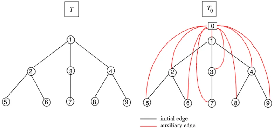
With the inclusion of adequate auxiliary edges in the original treeT, we transform the problem under study into a variation of the CMST problem (see, for instance,[13,14]). We note that a similar graph transformation has been suggested by Shaw[15]but, apparently, no reference to a modified CMST has been noted. Given the treeT , NandEas defined in Section 2, we define a new graphT0, obtained from T by adding a dummy node 0 and the edges(0, j )for each nodejinN, as described inFig. 1. Let, also, N0denote the set of nodes inT0 andE0the corresponding edge set.
The main idea of this transformation is to represent the situation “a concentrator is installed at node k” inT, by the situation “the edge(0, k)is included in the solution” inT0. The total demand served by that concentrator inT is represented by the flow in edge(0, k)inT0. Since the inclusion of each one of these
T T
1
2 3 4 2 3 4
5 6 7 8 9 6 7 8
0
1
5 9
initial edge auxiliary edge
0
1
2 3 4 2 3 4
6 7 8 6 7 8
5 9
initial edge expanded edge equipment
0
1
5 9
initial edge expanded edge auxiliary edge Feasible solution in T
Feasible solution in T0
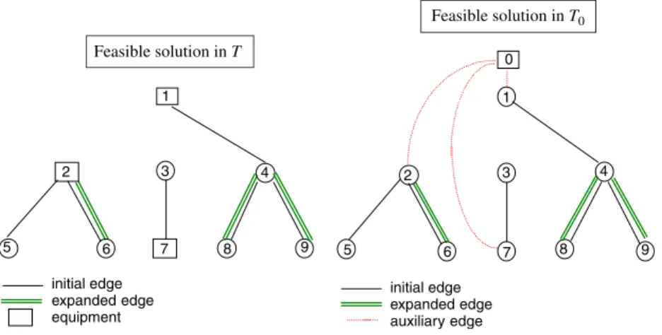
Fig. 2. Feasible solution forT andT0.
edges in T0 corresponds to the installation of one concentrator inT, the corresponding available edge capacity must be unlimited, and therefore these edges are not included in the set of edges to be expanded. Two costs are associated to the new edges(0, j ): one corresponding to the fixed cost of installation of one concentrator atj, Fj, and the other corresponding to the variable cost associated to the installation of
the concentrator, which depends on the flow that circulates through the edge.Fig. 2illustrates a feasible solution inT and the corresponding feasible solution inT0.
The alternative representation of the problem given by the new graph permits us to model the problem as a capacitated network flow model inT0. It is well known that network flow models have proven to be valuable in modelling many network design problems (see, for instance,[16]). It is also well known that a powerful modelling construct to improve formulations for several network design problems is to “direct the given network” (see[17–19]). Thus, we model our problem in a directed graph,D0=(N0, A0), as specified next. Each edge(i, j ) inE0 is replaced by two arcs, arci, jand arc j, i, with the same parameters as the original edge and we will denote byA0 the set of all arcs. Note, however, that each edge of the form(1, j )and(0, j )is replaced only by one single arc,1, jand0, j(we designate arc
0, jbyauxiliary arc).
3.1. Aggregated flow formulation
To define the aggregated flow-based formulation we use the following variables:
xij=
1 if arci, jis used,
0 otherwise, ∀i, j ∈A0,
yij=amount of flow circulating in arc i, j, ∀i, j ∈A0,
zij=
1 if arci, j is expanded,
0 otherwise, ∀i, j ∈A,
whereAis the arc set without the auxiliary arcs (note that these arcs are not expanded because we consider uncapacitated concentrators).
Our first model is the following directed flow-based formulation, which is denoted by FA0:
min
n
j=1
Fjx0j + n
j=1
cjy0j +
i,j∈A
Gijzij+
i,j∈A
eijsij,
s.t. (A1)
i:i,j∈A0
xij=1 ∀j ∈N,
(A2) zijxij ∀i, j ∈A,
(A3) yijBijxij+sij ∀i, j ∈A0,
(A4) sij(Mij−Bij)zij ∀i, j ∈A,
(A5)
i:i,j∈A0
yij−
i:j,i∈A
yji=dj ∀j ∈N,
(A6) yijsij ∀i, j ∈A,
(A12) xij∈ {0,1}, yij0 ∀i, j ∈A0,
zij ∈ {0,1}, sij0 ∀i, j ∈A. (FA0)
The objective function states that we want to minimize the sum of the concentrator costs together with all the link costs. Constraints (A1) ensure that each node, except node 0, has only one incident arc and constraints (A5) are the flow conservation constraints. Constraints (A2) ensure that an arc is expanded if it is used, constraints (A3) guarantee that the flow in any arc is less than or equal to the available capacity plus the added capacity and constraints (A4) give an upper bound on the added capacity. Note that, with (A3), (A4) and (A2), the flow that circulates in an arc is less than or equal to the maximum capacity of the arc, that is,yijMijxij, which we call “coupling constraints”. The two sets (A1) and (A5), together
with (A12) and the coupling constraints, guarantee that the set of arcs with correspondingx variables equal to 1 define a spanning tree.
Since the flow variablesyijrepresent the total demand that can circulate in arci, j ∈A(corresponding
to the sum of the initial flow with the one that use the added capacity), the total flowyijis greater than or
equal to the added capacity. Constraints (A6)yijsij,∀i, j ∈A, are not necessary for obtaining a valid
integer program but they are included as valid inequalities (in practice, the effect of these constraints on the lower-bound value of FA0 was very small—in our computer experiments, only in two cases were these constraints able to improve on the lower-bound value of FA0).
The formulation presented by Cho and Shaw [7]is equivalent to FA0 in terms of the corresponding linear programming relaxations. Instead of the two sets of variables,yijandsij, used in our model, they
one formulation into the other and prove that the corresponding linear programming relaxations are equiv-alent. It is, however, interesting to point out that in our computational experiments, our formulation has consistently produced smaller CPU times (one possible explanation for this is that the flow conservation constraints in Cho and Shaw’s formulation contain many more nonzero coefficients—due to the fact that they split variablesyijinto two sets of variables,yij1andsij).
As the results of Section 4 will show, the linear programming relaxation of FA0can be quite weak. We present next several sets of valid inequalities that improve the optimal solution of the linear programming relaxation of FA0.
Although the lower-bound inequality (A6) yijsij, ∀i, j ∈ A, is not effective in practice, we can
generate more effective inequalities based on the same concept of bounding below the flow in each arc. Note that if the amount of flow that passes through the arci, jis greater than the available capacity Bij, then it is necessary to expand the arc(zij=1)and the inequalityyijBijzijis valid. However, since
the flow that traverses each arci, jmust be greater than or equal to the demand in nodej (that is, the inequalityyijdjxijis also valid), we introduce the stronger inequality which subsumes the previous two
inequalities:
(A7) yijmax{Bij−dj,0}zij+djxij ∀i, j ∈A0.
To see the validity of (A7), consider the two cases: (i) ifzij=0 andxij=1 (the capacity of the arc is
not expanded) then we obtainyijdj, which is clearly valid (for the auxiliary arcs, this is the inequality
to include); (ii) ifzij=xij=1 (the capacity of the arc is expanded) then we obtainyijBij, which is also
valid (ifBijdj, then we haveyijdj).
A different set of lower-bounding inequalities is presented in Gouveia and Lopes[20]. In our case, we can use the fact that the input graph of the problem has a tree structure (and thus, the arcs that diverge from each node j are known). Let Sj be the subset of nodes that are endpoints of the arcs diverging from j. If these arcs are included in the solution, the minimum flow in arc i, jis equal to the sum of the demand of the nodes inSj. We introduce, then, the following new set of valid “lower-bounding” constraints:
(A8) yij
⎛
⎝dj +
k∈Sj
dk
⎞
⎠xij−
k∈Sj
dk(1−xj k) ∀i, j ∈A0.
To see that (A8) is valid we first consider the case|Sj| =1 (from[20]), that is, there is only one arc, say
j, k, diverging fromj. Suppose arcsi, jandj, kare in the solution. In this case, the minimum flow that crossesi, jmust be equal todj +dk (instead of being equal todj) because the flow in arci, j
must satisfy the demand of nodesj andk; that is,yij(dj +dk)xij−dk(1−xj k)is a valid inequality (see,[20]for the proof of its validity).
We note that the inclusion of (A8) does not necessarily imply that constraints yijdjxij become
redundant. To see this, note that when|Sj| =1, (A8) can be rewritten asyijdjxij−dk(1−xj k−xij)
and ifdk(1−xj k−xij) >0,yijdjxijis stronger than (A8).
To finish the discussion of valid inequalities for the aggregated formulation, we refer to two sets of valid inequalities introduced by Balakrishnan et al.[5]. In order to improve the lower-bound given by their formulation, Balakrishnan, Magnanti and Wong proposed valid inequalities relating the expan-sion of the network either with the installation of concentrators or with the expanexpan-sion of the links. To introduce these constraints, we first define the concept of saturated node: we say thatnode j is
satu-rated if the total demand in the subtree rooted at node j, which is denoted by D(j ), is greater than
the available capacity in the arc that connects the predecessor of j to j. Let Ns be the set of satu-rated nodes and, for each node j ∈ Ns, let aj be the predecessor of j and let T (j ) be the subtree rooted at j. Thus, for each saturated node, either we install one concentrator, at least, in the sub-tree rooted at j or we expand the arc that arrives into j. This argument leads to the first set of valid inequalities:
(A10)
k∈T (j )
x0k+zajj1 ∀j ∈Ns.
The other set of constraints guarantees that, if no concentrator is installed in the subtree T (j ), the capacity to add to that arc must be greater than or equal to the difference of the total demandD(j )and the available capacity of that arc, that is,
(A11) (D(j )−Bajj)
⎛
⎝
k∈T (j )
x0k
⎞
⎠+sajjD(j )−Bajj ∀j ∈Ns.
Constraints (A10) and (A11) are defined for each saturated node in the tree. We denote by FA1 the formulation FA0 augmented with (A7), (A8), with the simple two-subtour elimination inequali-tiesxij+xji1,∀(i, j ) ∈ E′ (these constraints are denoted by (A9) in the remainder of the text) and
the constraints based in saturated nodes (A10) and (A11)—some computational testing has shown that the optimal solutions of the linear programming relaxation of FA0 quite often violate several of these constraints.
3.2. Disaggregated flow formulation
The first disaggregated formulation, FD0, obtained directly from FA0with the new flow variables, is presented next:
min
n
j=1
Fjx0j + n
p=1
n
j=1
cjf0pj +
i,j∈A
Gijzij+
i,j∈A
eijsij
s.t. (D1)
i:i,j∈A0
xij=1 ∀j ∈N,
(D2) zijxij ∀i, j ∈A,
(D3)
n
p=1
fijpBijxij+sij ∀i, j ∈A0,
(D4) sij(Mij−Bij)zij ∀i, j ∈A,
(D5′)
i:i,j∈A0
fijp−
i:j,i∈A
fjip=0 ∀j, p∈N, p=j,
(D5′′)
i:i,j∈A0
fijj =dj ∀j ∈N,
(D6)
n
p=1
fijpsij ∀i, j ∈A,
(D13) fijpdpxij ∀i, j ∈A0, p∈N,
(D12) xij ∈ {0,1}, fijp0 ∀i, j ∈A0, p∈N,
zij∈ {0,1}, sij0 ∀i, j ∈A. (FD0)
The constraints that characterize this reformulation are the disaggregated flow constraints (D5′) , (D5′′) and the coupling constraints (D13)fijpdpxij,∀i, j ∈ A0,p ∈N. These constraints state thatxij=1
if arci, jcarries flow to any destination nodep.
Some of the constraints of the new model are taken from the aggregated model by simply substituting the aggregated variables yij with
n p=1f
p
ij (as the two sets of variables are related by the following
expressionyij=np=1f
p
ij). However, with the new variables, the direct substitution gives, sometimes,
redundant valid inequalities. For instance, it can be easily shown that constraints (D13) are satisfied as equalities whenp=jin the linear programming relaxation of FD0. This follows directly from constraints (D1) and (D5′′). Then, we haven
p=1f
p
ij f
j
ij =djxijimplying that the linear programming relaxation
of the disaggregated model is not improved by adding this constraint. Thus, the disaggregated inequality corresponding to (A7) becomes the simpler
(D7)
n
p=1
Using the relationship above between the two sets of variables, we can also prove (see[20]for a more general proof) that constraints (A8) rewritten with the new flow variables, that is, constraints
(D8)
n
p=1 fijp
⎛
⎝dj +
k∈Sj
dk
⎞
⎠xij−
k∈Sj
dk(1−xj k) ∀i, j ∈A0,
are redundant to the linear programming relaxation of FD0.
Finally, constraints (A9)xij+xji1,∀(i, j ) ∈ E′are also not considered in the new model because
they are also redundant in the corresponding linear programming relaxation. This follows from the fact that the projection into the space of the x variables, of the linear programming relaxation of (D1), (D5′), (D5′′), (D13) and (D12) gives a complete description of the convex hull of the incidence vectors of directed spanning trees (see, for instance, [19,22]). This description includes the so-called subtour elimination constraints and constraints (A9) are a small subset of this general class. We denote by FD1 the formulation FD0with the inclusion of (D7) and (A10) and (A11), the inequalities based in saturated nodes (these ones are not dependent of the new flow variables).
4. Computational tests
In the preceding sections, we have presented two classes of flow-based formulations for the local access network expansion problem: FA (aggregated flow formulations) and FD (disaggregated flow formula-tions). In this section, we present computational results that access their quality in solving instances of the problem. We also compare the use of such formulations with two formulations from Balakrishnan et al. [5]: the original one denoted by BMW0 and a strengthened version (denoted by BMW1), ob-tained from the previous one by adding the two sets of “saturated node” inequalities previously described and we also compare our methods with the pseudo-polynomial dynamic programming algorithm of Flippo et al.[8].
It should be pointed out that the BMW0 formulation involves index sets defining subsets of adequate feasible paths which permit to model the contiguity constraints and also permit the use of the “path-like” constraints to model the capacity constraints.
As we described in Section 2, the pseudo-polynomial dynamic programming algorithm of Flippo et al.
[8]has time complexity O(nB2)and requires O(nB)storage space, whereB is an upper bound for the concentrator capacity. As our problem considers uncapacitated concentrators, we make B equal to the total demand (as the authors of that paper suggest).
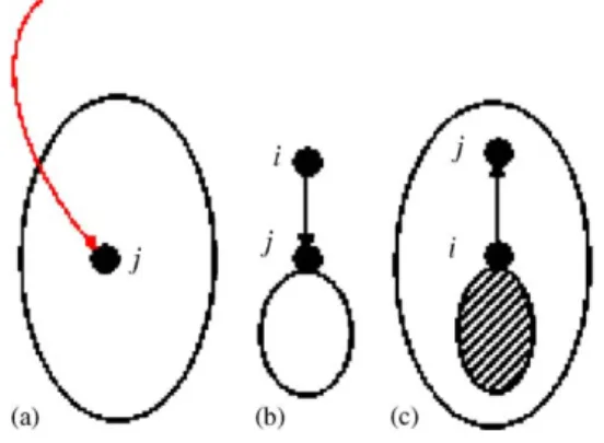
Fig. 3.Mijreduction (auxiliary,downandup arcs).
As another reduction test, note that ifMijBij, then the arci, jcannot be expanded and in an optimal
solution we must have zij =sij =0 (and these variables can also be eliminated). Note, however, that
this elimination rule is dependent on the value of theMijcoefficients. Thus, the elimination rule will get
stronger if these coefficients can be, somehow, reduced. Clearly, theMijcoefficients can be made equal
to the sum of all the node demands of the tree. However, this value is very poor and it can be improved in several ways. Let us consider the following three cases: (a) anauxiliary arc0, j, (b) adown arci, j
(the level of nodei is less than the level of nodej) and (c) anup arci, j(the level of nodej is less than the level of nodei), as illustrated inFig. 3.
In case (a), the value M0j can be made equal to the sum of all the demands that can be served by a concentrator located in nodej, that is, the demand of all the nodes of the subtree containingj. In case (b), the valueMijcan be made equal to the maximum flow traversing that arc which is the total demand
of the downstream nodes (if the arc is used and as the network has a tree structure, there is no way to send flow to a node situated above nodej). The flow that traverses an up arc (case (c)) can only go to the nodes belonging to the same subtree but not belonging to the subtree rooted atiand, thus,Mijcan be
made equal to the corresponding demand.
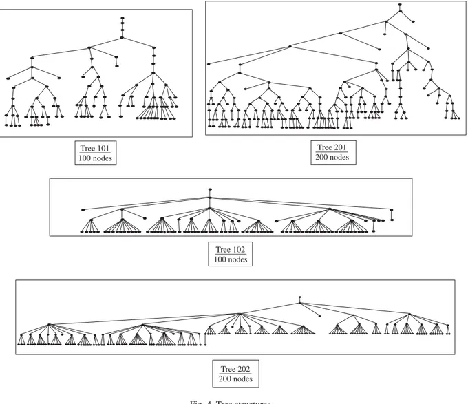
In order to evaluate and compare the corresponding linear programming relaxations, we have generated several instance problems with different parameters. As stated before, the networks involved have a fixed tree structure. We have performed our tests with trees involving 100 and 200 nodes. We have generated two 100-node instances and two 200-node instances, where the number of sons for each node is less than or equal to 3 (tree 101 and 201) and less than or equal to 10 (tree 102 and 202).Fig. 4summarizes the tree topologies of the instances tested. We have used the same trees with different parameters to generate new instances. For each problem instance we have considered four more additional cases: we have divided the demand of each node by 5 and 2, respectively, and have multiplied it by 2 (these three types of instances are denoted by P/5, P/2 and P×2, respectively). The fourth case is obtained by doubling the fixed cost of the concentrators (instances denoted by F×2). InTable 1, we present the results for all the instances: the four new instances as well as the original ones.
The table depicts the gaps given by the optimal linear programming bound of the models and the CPU times. The first two columns specify the instance problems. The next 12 columns present the gaps given by the optimal linear programming bound of the models; each model has two columns associated, denoted
Tree 101 100 nodes
Tree 201 200 nodes
Tree 202 200 nodes Tree 102 100 nodes
Fig. 4. Tree structures.
Results for instances with 100 and 200 nodes (trees presented)
Tree Prob. FA0 FA1 FD0 FD1 BMW0 BMW1 Flippo et al. (B) Optimum
With Without With Without With Without With Without With Without With Without
101 P/5 4.45(0+2) 5.85(0+39) 1.84(0+1) 2.04(0+3) 1.70(0+6) 1.71(2+48) 1.28(0+3) 1.29(2+55) 2.61(0+0) 4.49(1+10h) 1.83(0+0) 3.55(1+10h) 3 (2459) 282526 P/2 1.97(0+0) 5.40(0+1) 0.58(0+0) 1.12(0+0) 0.77(0+0) 1.05(1+6) 0.48(0+0) 0.82(1+7) 1.71(0+0) 5.23(0+10h) 1.0(0+0) 4.01(1+17557) 12 (6174) 745118 P 0.27(0+0) 4.12(0+0) 0.04(0+0) 0.19(0+0) 0.05(0+0) 0.19(1+3) 0.04(0+0) 0.18(1+3) 0.37(0+0) 4.17(0+582) 0.28(0+0) 3.04(1+497) 44 (12297) 1515179 P×2 0.13(0+0) 2.32(0+0) 0.01(0+0) 0.05(0+0) 0.03(0+0) 0.05(1+2) 0.01(0+0) 0.05(1+2) 0.19(0+0) 2.40(0+5719) 0.07(0+0) 1.88(0+30) 84 (24594) 3031686 F×2 0.45(0+0) 5.30(0+0) 0.06(0+0) 0.24(0+0) 0.09(0+0) 0.24(1+2) 0.06(0+0) 0.23(1+2) 0.55(0+0) 4.45(0+3516) 0.45(0+0) 3.24(1+554) 43 (12297) 1534286
102 P/5 5.61(0+2) 6.18(0+3) 2.25(0+1) 2.36(0+1) 1.04(1+24) 1.04(1+29) 0.88(1+17) 0.94(1+37) 5.69(0+47) 6.23(1+2793) 4.87(0+43) 5.49(1+2608) 2 (2207) 245151 P/2 2.23(0+0) 5.22(0+1) 0.72(0+0) 0.96(0+1) 0.76(0+1) 0.84(1+8) 0.46(0+1) 0.55(1+6) 1.69(0+0) 5.22(0+10h) 0.68(0+0) 2.73(1+308) 11 (5540) 649575 P 0.85(0+0) 4.08(0+0) 0.19(0+0) 0.24(0+0) 0.25(0+0) 0.26(1+4) 0.18(0+0) 0.20(1+3) 0.95(0+0) 4.20(0+412) 0.61(0+0) 1.63(0+82) 38 (11032) 1329866 P×2 0.42(0+0) 2.77(0+0) 0.02(0+0) 0.04(0+0) 0.07(0+0) 0.08(1+1) 0.02(0+0) 0.04(1+1) 0.49(0+0) 3.06(0+24) 0.17(0+0) 1.56(0+18) 73 (22064) 2686910 F×2 0.97(0+0) 5.38(0+1) 0.22(0+0) 0.28(0+0) 0.29(0+0) 0.31(1+3) 0.21(0+0) 0.22(1+4) 0.95(0+0) 4.48(0+550) 0.63(0+0) 1.77(0+138) 39 (11032) 1348428
201 P/5 4.24(1+5921∗)5.77(0+10367∗)1.90(0+180)2.01(0+1596)1.56(1+848) 1.58(13+10h)1.26(1+1261) 1.28(19+10h)2.25(0+4) 4.20(5+10h) 1.77(0+2) 3.32(5+10h) 9 (3964) 446812 P/2 2.30(0+1) 5.51(0+22) 0.69(0+0) 0.90(0+2) 0.83(0+0) 0.86(10+67) 0.63(0+0) 0.70(11+145) 2.07(0+0) 5.31(4+10h) 1.52(0+0) 4.17(4+10h) 49 (9955) 1188796 P 0.62(0+0) 4.54(0+2) 0.14(0+0) 0.25(0+0) 0.21(0+0) 0.26(9+37) 0.14(0+0) 0.20(8+34) 0.71(0+0) 4.73(3+19943∗)0.29(0+0) 3.66(4+24766∗)172 (19805) 2430117 P×2 0.13(0+0) 2.77(0+1) 0.02(0+0) 0.03(0+0) 0.03(0+0) 0.03(7+30) 0.02(0+0) 0.02(8+28) 0.13(0+0) 2.80(3+21039∗)0.06(0+0) 2.12(3+22805∗)332 (39610) 4880740 F×2 0.82(0+0) 5.87(0+3) 0.13(0+0) 0.28(0+1) 0.23(0+0) 0.28(10+33) 0.13(0+0) 0.20(9+35) 0.82(0+0) 5.03(4+1611∗) 0.29(0+0) 3.89(4+23162∗)172 (19805) 2464688
202 P/5 5.28(0+6730) 6.01(0+9175∗) 1.42(0+90) 1.49(0+109) 1.11(7+23765)1.12(11+10h)0.84(9+12668)0.84(11+9413)4.37(1+10h)6.03(19+10h) 3.40(1+10h)4.48(8+10h) 11 (4133) 476431 P/2 2.27(0+1) 4.91(0+9) 0.47(0+0) 0.78(0+1) 0.50(0+2) 0.52(11+61) 0.35(0+3) 0.36(8+43) 1.66(0+1) 5.21(9+10h) 1.14(0+1) 3.09(9+10h) 62 (10390) 1257610 P 0.88(0+0) 4.06(0+2) 0.09(0+0) 0.17(0+0) 0.16(0+0) 0.16(10+7) 0.09(0+0) 0.10(9+4) 1.0(0+0) 4.35(9+10h) 0.70(0+0) 2.32(9+10h) 231 (20679) 2565873 P×2 0.29(0+0) 2.69(0+1) 0.05(0+0) 0.06(0+0) 0.08(0+0) 0.08(6+15) 0.05(0+0) 0.06(6+17) 0.33(0+0) 2.96(6+10h) 0.17(0+0) 1.70(5+4380) 449 (41358) 5170607 F×2 1.49(0+0) 5.45(0+2) 0.12(0+0) 0.25(0+1) 0.19(0+0) 0.19(10+7) 0.10(0+0) 0.10(8+6) 1.44(0+0) 4.65(10+10h) 0.91(0+0) 2.50(6+10h) 230 (20679) 2603898
As expected, the disaggregated flow formulations FD produce, in general, the better linear programming bounds. However, it is interesting to see that FD0improves a lot over FA0but the same does not happen when we examine the formulations FD1 and FA1 (with or without pre-processing). This suggests that disaggregating the models gets substantially less effective after adding some of the valid inequalities to the models.
We present the results with and without pre-processing to see the influence that pre-processing has in the results. In all cases, without pre-processing, we have higher gaps because pre-processing eliminates many variables and reduces quite effectively theMijcoefficient. Although variable elimination and coefficient
reduction are done, in many cases, more than once, the time pre-processing takes in all instances considered is less than 1 s.
The CPU times of the FA and FD models are insignificant for almost all cases, with and without pre-processing. The exception is for instances P/5 (with small demand) with 200 nodes, where CPU times are more significant. We see also that, for each instance, the gaps decrease when demand increases.
The gaps given by the BMW model are in general worse than the ones produced by the models FA and FD. Note also that BMW model involves many more variables and constraints (this is a consequence of the previously mentioned index sets that define the paths in the tree). However, pre-processing has a great impact in this model because it eliminates many paths, leading to reduced CPU times (the exception is again the instance with 200 nodes and demand P/5) and reduced gaps; without pre-processing, the CPU times of the BMW models are very high. We can also see that within each class, the more complicated models (the models with more inequalities) do not take substantially more time than the original models (in some cases they take less time, namely without pre-processing).
For the instances with the fixed cost of concentrators multiplied by 2, the CPU times are more or less the same when comparing with the original instance. However, the gaps increase a little because the costs encourage the installation of concentrators instead of expanding the links (with the increase of the fixed cost, this behaviour is not significant).
We have also tested the instances with the pseudo-polynomial algorithm developed by Flippo et al. [8].The results show that FA models and the pseudo-polynomial algorithm have inverse behaviours; the FA models produce worse results when demand is smaller (corresponding to a smaller value for B); Flippo’s algorithm is clearly favoured for the instances with small B (because its running time increases when B increases). This becomes very clear in the 200 node instances and the demand divided by 5 (solving the integer models takes much more time than using their algorithm). How-ever, our experiments also indicate that for instances with the same number of nodes and higher de-mand, the FA models are solved within 2 s (with pre-processing) and the algorithm needs up to 50 and 450 s.
As the pre-processing has a great influence in our instances and our trees have a great number of saturated nodes, we decided to test the models with other instances. Since Flippo et al. [8]made available their instances, we decided to test their instances with 100 and 200 nodes (see[8], for instances characteristics). However, they have used their algorithm in instances with different capacities for the concentrators. As our problem considers uncapacitated concentrators, we need to adapt the instances making the valueB equal to the total demand of the tree.
Corte-Real,
L.
Gouveia
/
Computer
s
&
Oper
ations
Resear
ch
34
(2007)
1141
–
1157
1155
Table 2
Results for instances with 100 and 200 nodes (Flippo et al. instances)
Tree FA0 FA1 FD0 FD1 BMW0 BMW1 Flippo et al. (B) Optimum
With Without With Without With Without With Without With Without With Without
LANEP100a 15.67(0+0) 15.97(0+0) 0.25(0+0) 0.25(0+0) 1.40(0+1) 1.40(1+0) 0.10(0+1) 0.10(1+0) 4.21(0+7) 4.23(0+15) 2.30(0+7) 2.32(0+13) 20 (5519) 148682 LANEP100b 20.69(0+0) 21.42(0+0) 2.25(0+0) 2.27(0+0) 2.31(0+2) 2.31(0+1) 0.51(0+1) 0.51(0+1) 4.38(0+4) 4.43(0+12) 2.57(0+5) 2.61(0+11) 12 (4999) 178068 LANEP100c 13.18(0+0) 13.28(0+0) 0.33(0+0) 0.33(0+0) 1.54(1+0) 1.54(1+0) 0.12(1+0) 0.12(1+0) 3.61(0+18) 3.66(0+37) 2.08(0+19) 2.13(1+37) 20 (5213) 250237 LANEP200a 11.24(0+0) 13.60(0+0) 0.55(0+0) 0.55(0+0) 2.18(2+1) 2.19(2+3) 0.08(2+1) 0.08(2+1) 3.76(1+78) 3.90(2+181) 1.65(1+59) 1.66(3+135) 170 (10364) 194371 LANEP200b 10.21(0+0) 10.98(0+0) 0.22(0+1) 0.22(0+0) 2.03(2+2) 2.03(2+3) 0.06(2+1) 0.06(2+2) 4.53(1+38) 4.60(3+163) 2.36(1+40) 2.48(3+203) 168 (10115) 255752 LANEP200c 10.90(0+0) 12.17(0+0) 0.42(0+0) 0.42(0+0) 2.07(2+1) 2.07(2+1) 0.18(2+0) 0.18(2+1) 4.53(1+29) 4.53(2+80) 2.62(1+30) 2.62(3+81) 122 (10282) 252691 LANEP200d 10.26(0+0) 10.48(0+0) 0.46(0+1) 0.46(0+0) 1.43(2+3) 1.43(3+2) 0.03(3+0) 0.03(3+0) 2.51(1+59) 2.52(2+171) 1.08(1+61) 1.09(7+194) 165 (9838) 267474
Lan100a 4.38(0+0) 4.79(0+0) 1.38(0+0) 1.67(0+0) 1.29(0+1) 1.29(0+2) 1.24(0+0) 1.24(0+1) 7.54(0+1) 7.55(0+25) 6.17(0+1) 6.25(0+4) 2060 (155886) 90157699 Lan100b 1.84(0+0) 2.38(0+0) 0.13(0+0) 0.13(0+0) 0.06(0+0) 0.17(0+1) 0.02(0+0) 0.02(0+1) 3.61(0+0) 4.92(0+8) 3.18(0+0) 4.12(0+8) 1455 (150503) 104116914 Lan100c 5.45(0+0) 5.67(0+0) 1.95(0+0) 2.45(0+0) 0.12(0+0) 0.12(1+1) 0.02(0+0) 0.02(1+1) 8.28(0+1) 8.76(0+51) 7.65(0+1) 8.17(0+43) 2672 (153395) 114187229 Lan100d 2.67(0+0) 3.42(0+0) 0.52(0+0) 0.86(0+0) 0.26(0+0) 0.35(1+1) 0.16(0+0) 0.25(1+1) 6.75(0+1) 7.94(0+47) 6.08(0+0) 6.85(0+15) 3346 (141653) 80395979 Lan100e 3.64(0+0) 3.78(0+0) 0.83(0+0) 1.41(0+0) 0.28(0+1) 0.28(1+2) 0.26(0+0) 0.26(1+2) 7.23(0+1) 7.35(0+53) 6.85(0+1) 6.98(0+22) 2449 (142890) 81913205 Lan200a 2.23(0+1) 2.65(0+1) 0.60(0+0) 1.0(0+1) 0.17(1+3) 0.19(7+24) 0.12(1+3) 0.12(10+21) 6.19(0+6) 6.91(3+3520) 5.68(0+5) 6.33(3+363) 28438 (296660) 177869617 Lan200b 3.38(0+1) 3.98(0+2) 1.40(0+1) 1.5(0+1) 0.58(0+1) 0.59(2+9) 0.47(0+1) 0.48(3+7) 6.13(0+3) 6.63(1+161) 5.13(0+3) 5.42(1+244) 18828 (299731) 208825278 Lan200c 4.19(0+0) 4.92(0+1) 0.73(0+0) 1.16(0+1) 0.55(0+1) 0.55(9+27) 0.27(0+1) 0.27(12+22) 6.84(0+4) 7.79(4+6923) 5.76(0+3) 6.48(4+2030) 22199 (289728) 220815561 Lan200d 2.74(0+0) 3.32(0+1) 0.42(0+0) 0.43(0+1) 0.18(0+3) 0.18(3+13) 0.08(1+1) 0.08(4+16) 4.22(0+6) 4.81(1+231) 2.57(0+4) 3.10(3+134) 24916 (290630) 202371438 Lan200e 3.25(0+1) 3.79(0+1) 1.20(0+0) 1.43(0+1) 0.66(0+3) 0.67(14+20) 0.56(1+1) 0.57(16+23) 6.19(0+8) 7.17(4+10h) 5.66(0+9) 6.24(5+5848) 18272 (277249) 217420459
present a column giving the CPU time that Flippo’s algorithm needs to solve the corresponding instance. The last column gives the optimal value.
The first remark is that the CPU time is very small for FA and FD models. Only for BMW model, it is, in some cases, higher. Our models always use less CPU time than Flippo’s algorithm (for the FA model, the CPU times are not greater than 2 s). However, the average gaps are, in general, higher than the average gaps in the instances generated by us.
With the inclusion of valid inequalities, the linear programming gaps decrease considerably. Comparing the more complicated model within each class, with pre-processing, there are higher gaps in BMW1 (in average, 4.1%) but much lower in FA1and FD1; in the first case, the gaps are less than 2% (the exception is the instance LANEP100b, with gap value given by 2.25%) and in the second, less than 1% (the exception is the instance Lan100a, with gap value given by 1.24%).
With respect to the disaggregated models FD0 and FD1 we notice that the pre-processing is not so significantly as in our instances, in terms of time and gaps (furthermore, in some cases gaps are equal with and without pre-processing).
To conclude this section, we make a brief remark to the work by Balakrishnan et al.[5]and the algorithm developed by Flippo et al.[8]. We have given empirical experiments showing that our network flow-based methods seem preferable to BMW model, when we use CPLEX as a solving tool. We note, however, that the paper by Balakrishnan et al.[5]also describes a lagrangian relaxation based on their formulation and with the property that the associated lagrangian dual bound is better than the corresponding linear programming bound. Thus, their lagrangian bounds should be better than the lower bounds reported here in the columns corresponding to BMW models. With respect to the pseudo-polynomial algorithm, our models appear, in general, to be preferable to the algorithm developed by Flippo et al. [8]. However, as we said before, the problem under study where concentrators have no capacities corresponds to the worst-case behaviour of their algorithm.
Nonetheless, we still believe that the network flow-based approach here proposed is worth trying as our results show that we can solve quite easily instances with up to 200 nodes.
Acknowledgements
We thank the authors of[8]by making their instances and algorithm available.
References
[1] Balakrishnan A, Magnanti TL, Shulman A, Wong RT. Models for planning capacity expansion in local access telecommunication networks. Annals of Operations Research 1991;33:239–84.
[2] Gavish B, Helme M, Kai SR. Concentrator placement and link expansion in local access networks. Working paper, GTE Laboratories, Waltham, MA, 1988.
[3] Bienstock D. Computational experience with an effective heuristic for some capacity expansion problems in local access networks. Telecommunication Systems 1993;1:379–400.
[4] Lee CY. An algorithm for the design of multitype concentrator networks. Journal of Operational Research Society 1993;44(5):471–82.
[6] Cho G, Shaw DX. Limited column generation for local access telecommunication network expansion and its extensions—formulations, algorithms and implementation. Technical Report, School of Industrial Engineering, Purdue University; 1996.
[7] Cho G, Shaw DX. Models and implementation techniques for local access telecommunication network design. In: G. Yu, editor. Industrial applications of combinatorial optimization, 1998.
[8] Flippo OE, Kolen AWJ, Koster AMCA, Leensel RLMJ. A dynamic programming algorithm for the local access telecommunication network expansion problem. European Journal of Operational Research 2000;127:189–202. [9] Jack C, Kai S-R, Shulman A. Netcap—an interactive optimization system for GTE telephone network planning. Interfaces
1992;22(1):72–89.
[10] Jack C, Kai S-R, Shulman A. Design and implementation of an interactive optimization system for telephone network planning. Operations Research 1992;40(1):14–25.
[11] Shulman A, Vachani R. A decomposition algorithm for capacity expansion of local access networks. IEEE Transactions on Communications 1993;41(7):1063–73.
[12] Magnanti TL, Mirchandani P, Vachani R. Modeling and solving the two-facility capacitated network loading problem. Operations Research 1995;43(1):142–57.
[13] Gavish B. Formulations and algorithms for the capacitated minimal directed tree problem. Journal of the Association for Computing Machinery 1983;30(1):118–32.
[14] Gouveia L. A comparison of directed formulations for the capacitated minimal spanning tree problem. Telecommunications Systems 1993;1:51–76.
[15] Shaw DX. Reformulation, column generation and Lagrangian relaxation for local access network design problems. Technical Report, 1994.
[16] Magnanti TL, Wong RT. Network design and transportation planning: models and algorithms. Transportation Science 1984;18:1–55.
[17] Balakrishnan A, Magnanti TL, Mirchandani. Modeling and heuristic worst-case performance analysis of the two-level network design problem. Management Science 1994;40(7):846–67.
[18] Goemans MX, Myung Y. A catalog of Steiner tree formulations. Networks 1993;23:19–28.
[19] Magnanti TL, Wolsey L. Optimal trees in network models. In: Handbooks in operations research and management science, vol. 7, 1995. p. 503–615.
[20] Gouveia L, Lopes MJ. Valid inequalities for non-unit demand capacitated spanning tree problems with flow costs. European Journal of Operational Research 2000;121:394–411.
[21] Rardin R, Choe U. Tighter relaxations of fixed charge network flow problems. Report 3-79-18, Industrial and Systems Engineering, Georgia Institute of Technology, Atlanta, 1979.