Phase topology and percolation in two-component lipid bilayers: A Monte Carlo approach

Biophysical Journal Volume72 April 1997 1501-1511

Phase

Topology

and

Percolation

in

Two-Component Lipid

Bilayers:

A

Monte

Carlo Approach

Fernando P. Coelho,* Winchil L. C. Vaz,# and Eurico Melo*

Instituto deTecnologiaQuimicaeBiologicaand IST, Apartado 127, P-2780Oeiras,and#UnidadedeCienciasExactaseHumanas,

Universidade doAlgarve,CampusdeGambelas, P-8000Faro, Portugal

ABSTRACT MonteCarlo simulations of fluorescencerecovery afterphotobleaching(FRAP)experimentsontwo-component lipid bilayerssystems in thesolid-fluid phase coexistence region were carried out to studythe geometryand size of fluid

domains inthese bilayers.Thegel phasewassimulated bysuperposableelliptical domains, whichwereeitherof

predeter-mined dimensions, increasing in number with increasing gel phase fraction, or of predetermined number, increasing in dimensions with increasing gel phasefraction. The simulations were done from two perspectives: 1) atime-independent analysis offractional fluorescence recovery as afunction of fractional fluid phase in thesystem; and 2) atime-dependent

analysis of fractional fluorescence recovery as a function of time at a given fraction of fluid phase in the system. The time-dependentsimulations result inrecovery curves that aredirectlycomparabletoexperimentalFRAPcurvesandprovide topological andgeometrical models for thecoexisting phasesthat are consistent with theexperimental result.

INTRODUCTION

Phospholipid bilayers composed of binary lipid mixtures form nonideal mixtures thatexhibitphaseseparationover a

large range of temperatures at constant pressure(Shimshick

and McConnell, 1973; Wu and McConnell, 1975; Mabrey

andSturtevant, 1976).Wewill beconcernedhere withrigid

andfluid coexistingphases, buttwodifferent liquid phases

may aswell besimultaneouslypresent in abilayer (Almeida

et al., 1992a). These two phases form a mosaic of

micro-scopic phase domains whose long-term stability, although

controversial from the theoreticalviewpoint(Mouritsen and

J0rgensen, 1994),hasbeen observedexperimentally (Vazet

al., 1989). An important question concerning the bilayer

structure in the region of phase coexistence concerns the

topology of the phasesin equilibrium. Notably, the lateral

organization of the domains in each phase of a bilayer in this physical state may control the kinetics and yield of chemical processes occurring between membrane compo-nents(Melo etal., 1992). These components must percolate toward each other to allow collisional interaction.

There-fore, when because of physical or chemical conditions a

phase separation is developedin the membrane, the

possi-bility and characteristics ofthe molecular percolation

be-comeimportantreaction parameters(Meloetal., 1992;Vaz, 1992; Vaz andAlmeida, 1993).

For a given composition, bydecreasing the temperature from above to below theliquidus line, theformationof the gel phase will take place at the cost of the fluid (the system enters thetwo-phase solid-liquid coexistence region). In the

initially completely homogeneous liquid phase, isolated

Receivedfor publication28 October1996 and infinalform 10January

1997.

Address reprint requests to Dr. Eurico Melo, Instituto de Tecnologia,

QuimicaeBiol6gica,Apartado127, P-2780 Oeiras, Portugal. Tel.: 35 1-1-441-7823; Fax: 351-1-442-1161;E-mail:[email protected].

© 1997bytheBiophysicalSociety

0006-3495/97/04/1501/11 $2.00

soliddomains appear at some nucleationpoints as a minute fraction of the total mass. As the temperature is decreased, more gel phase is inducedto form. A givenphase is con-sidered to be percolating when a continuous cluster of its domains allows thetracing of a path across the entire system without leaving this phase (Stauffer and Aharony, 1994). Therefore, even if some regions of fluid may be, at this stage, isolated from the bulk fluidfraction, at least part of it is continuous and the system is still defined as percolating.

Extrapolating whatis observed inLangmuir-Blodgettfilms to our system, the increase in the fractional mass of solid may occur via the growth of the existing

rigid

domains withoutchanging the number ofdomains, orbynucleating new domains, orboth (Markov, 1995). In any case, aswe

approach the solidus line, fora given composition, perco-lation in the fluid phase is lost and the solid becomes continuousoverlargerdistances. Thefluidfractionatwhich the liquid phase becomes disconnected is known as the

percolation threshold, pc (Stauffer and Aharony, 1994; Saxton, 1987).

Thepercolation thresholddefinesanimportant inflection point in thekineticsand theyieldof reactions between those membraneproteinsand/or other reactant species essentially insoluble in solidphases (Melo et al., 1992). Whereas below thepercolation threshold theirdiffusionwill beconfined to isolated liquid domains of heterogeneous geometry and area,immediatelyabove the percolationpoint the number of

available reactants per domain increases rapidly, although their free diffusion in the membrane plane is stillrestricted bytherigiddomains. These facts may have consequences at various levels for the biological processes in a membrane because of the forced reactant isolation or thehindrance of theirdiffusion (Vaz, 1996). Infact,it is thetopology of the

coexisting phases that, in this case,conditions the rate and the chemical yieldof thebiochemical processes.

To try to understand and model the consequences of

phase separation in the reactions occurring in the

branes, especially from the kinetic viewpoint, it is essential to have information concerning the structure and

dimen-sions ofthephase-separated domains. However, the pattern of the fluid and gel domains in a membrane has never been directly observable by conventional optical microscopy, presumably because the dimension of the domains falls below the resolutionof the technique (-A/2).Therefore, if we want to access the topology of the phase-separated membrane, either a better resolution is needed, or indirect methods must be employed. Some high-resolution

tech-niques such as electron microscopy (Hui, 1981), atomic force microscopy (Radmacher et al., 1992), and near-field

scanningoptical microscopy (Hwang et al., 1995) have been used with varying success, and we will have to await

refinementsbefore their utility can be clearly assessed. The objectiveofthe present work is to discuss possible geomet-rical arrangements of the fluid-rigid mosaic that are com-patible with the experimental findings concerning molecular

diffusion in these systems obtained from the fluorescence

recovery after photobleaching (FRAP) technique.

Vaz etal. (1989) showedforthe first time how the FRAP

techniquecould be used todetermine the percolation thresh-old inphospholipidbilayers. In that work thediffusion ofa fluorescent tracermolecule, only soluble in thefluidphase

ofatwo-phase fluid-solid coexistence system, wasstudied,

and thismadeitpossibletodraw some conclusions

regard-ing in-plane percolation in these membranes. Since then several systems have been studied with the same method

(Vaz et al., 1990; Bultmann et al., 1991; Almeida et al.,

1992b).

In a FRAPexperiment, if free diffusion occurs overthe entire area ofthe membrane beingexamined, andthe illu-minated area is only a very small fraction of the total membrane area, the measured fluorescenceintensityat

"in-finite"time after the photobleaching pulseattains the value measuredbeforethe pulse. Incomplete fluorescence

recov-ery is symptomatic of immobilization of the fluorescent

probes in the membraneplane duringthe timeofthe exper-iment. If the fluid-phase domains areofa size comparable

to the photobleached area, a sharp change in the recovery

fractionatthepercolation threshold isnotobserved. Instead,

ifwe represent the fraction of fluorescence recovery as a

function of thefraction ofareaof thefluidphaseforagiven

phase-separated phospholipid system, weobtain a sigmoid

curve. Assuming that the FRAP fractional fluorescence

recovery represents the probability of percolation of the liquid phase in the membrane underinvestigation,Almeida

etal. (1992b, 1993) concluded that the systempercolation

threshold should be defined by the inflection point of the

curve.

If the diffusion in the phase-separated lipid bilayer is viewed as aproblem of continuum percolation in two

di-mensions, the percolation threshold, defined as the

mini-mum liquid area fraction for whichthis phase is still

con-tinuous,can

give

an

insight

into the

shape

of the

solid-phase

domains (Xia and Thorpe,

1988).

However,

to be able to

continuum percolation theory, an a priori definition of the geometric elements with which the rigid phase is build becomes necessary. One possible model representing the gel-phase elements as ellipses with aspect ratiobla has been thoroughly studied by Xia and Thorpe (1988) and will be

designated hereafter asthefixed-ellipse model. Within the contextofthis model, the solid domain structure would be characterized by a random distribution of identical ellipses that may superimpose in each bilayer sheet. Differences in

the gel-phase fraction arise from varying the number of ellipses per unit of membrane area without changing the geometric characteristics ofthe ellipses. It is important to recall that, as Xia et al. have demonstrated, the percolation threshold,

pc,

is afunction of the ellipse aspect ratio, b/a, and so,foragiven experimentalpcvalue itwillbepossible to estimate b/a. Besides, this relation between pc and b/a being highly convenient, the useofellipsesis quite

reason-able, at least when the fraction of solid phase is small,

because in monolayers the crystalline domains present an

ellipse-like shape (Kelleretal., 1987). Although this

treat-mentallows an estimationof thesolid-domainshape,itdoes notgive any clue concerningits absolute sizeorthe shape and size ofthecoexistent fluiddomains.

Inan attemptto evaluate the average size ofthe

phase-separated domains, Almeida et al. (1993) have deduced a

relationshipbetween thefractionalrecoveryof fluorescence

at equilibrium after photobleaching, the fractional area of thefluidphase,and the ratiobetween thelinear dimension ofthefluiddomains and the radius ofthe FRAPbleaching

spot.Thistreatmentpresupposesthat itispossibletoderive the exact value of the fractional fluorescence recovery at

equilibrium after photobleaching from the experimental

curves.

In this work we present a MonteCarlo simulation ofthe

percolation problem in biphasic (solid-fluid coexistence) lipid bilayers. We have used the

fixed-ellipse

model,

re-ferred to above, in these simulations. Afirst phase of this

work attempted to reproduce experimental plots of

frac-tional fluorescence recovery at equilibrium after photo-bleachingversusfluidfractionof the system. Agreementof the simulations with theexperimentalpointswasobtainedat

values above thepercolation thresholdofthe system with significant discrepancy close to or below the

percolation

threshold. This suggested that the dimensions of the fluid domains relative to the radius of the FRAP spot were reasonably well estimatedbythe model.

In a second phase of this work we attemptedto under-stand the discrepancy between the model-derived simula-tionsand theexperimental results. The

experimental

values of the fractional fluorescence recovery are

essentially

a

result ofinterpretationof therawdata,andit may be

argued

that a betterprocedure wouldbe to simulate the

complete

experimental curves in the time domain. In

practice,

the

experimental recoverycurves in the

region

of

phase

coex-istence cannot be fitted with the normal solution of the

equationforhomogeneous diffusion in two dimensions, as

Topology of Phase-Separated Bilayers because they exhibit an anomalous tail in the long-time

regime just above and below the percolation threshold. In previous work, to obtaina goodfit, we artificiallyadded a "linearramp"to theconventional solutionexpression (Vaz

et al., 1989, 1990; Bultmann et al., 1991; Almeida et al.,

1992b). Thisartificewasbased on theinterpretationthat the slowdiffusioncomponentwasdueto tracerdiffusionin the

gel-phase defects,witharecoverytime thatwasslowonthe

time scaleofourFRAPexperiment, thuspermitting approx-imate description by a straight line superimposed on the

fluid diffusion component. The extremely good fits ob-tained (an example ofwhich ispresentedinFig. 1) do not

dismiss other interpretations, including one in which the

slow componentis inherent to diffusion withpercolation.

An alternative analysis of the FRAP experimental data canbeachieved by utilization ofthefixed-ellipsemodel in a Monte Carlo simulation in the time regime. Within the contextof the continuum percolation model, the simulated FRAP curves are obtained, assuming that thelateral diffu-sion ofthe tracer molecules in the FRAPexperimentcanbe treatedas arandomwalk on atwo-dimensional obstructed

continuum. Theimpenetrableobstacles may berepresented byrandominclusion ofsuperimposable elliptical structures

of uniform area, asdescribedearlier.The fit of the simula-tionresults to theexperimentaltime-resolved FRAPcurves

should thenprovidetheidealdomain geometry and

dimen-sionswithinthecontextofthe model. Thisprocedure, with which only diffusion ofthe probe in the liquid phase is

reported, can be used to verify whether the referred long time tailis actually associated withdiffusioningeldefects

or whether it is related to an anomalous diffusion in a

percolating system. 1.0 0.8- 0.6-0 0.4 -( 0.2-0.0 0 5 10 15 20 25 30 time(s)

FIGURE 1 Fit of experimentaltime-dependent FRAP recovery data for theDMPC/DSPC(50/50) systemat34.9°C, p =0.47 (noisy curve) (Vaz

etal.,1989). Thesmooth curvesrepresentbestfits to the experimental data, usingtheexpression derived by Soumpasis (1983) with and without adding

a"linearramp"(solid and dotted lines, respectively). In the first case the bestfitwasobtained with fittingparameters TD = 1.02 s,F(0) = 2904

counts,F(oo) = 6560 counts, slope of "linear ramp"=21.3 counts/s, and

thegoodness-of-fitparameterx2=1.3. For the second case the parameters

areTD=1.99,F(0)=3238 counts, F(o)=7151 counts, andv= 1.9. All

curves arenormalized.

Fluid- and solid-domain topologies being

complemen-tary, from the above simulations we obtain the necessary information about the geometry of the fluid domains near or below thepercolation threshold, a region where such infor-mation may be of fundamental biological interest, particu-larly with respect to molecularinteractions between diffus-ing reactants (Melo et al., 1992).

We are not the first to attempt an evaluation of the averagedomain sizes inbilayersconstituted of mixed phos-pholipids. A first attempt has been presented by Sankaram etal.(1992)for mixed

1,2-dimyristoyl-sn-glycero-(3)-phos-phocholine (DMPC)/1,2-distearoyl-sn-glycero-(3)-phos-phocholine (DSPC) bilayers. From an electron spin reso-nance study these authors conclude that the disconnected liquid crystalline domains are onthe order of several hun-dred lipid molecules, although they admit that larger

do-mains arepossible (Sankaramet al., 1992). In a computer simulation of FRAP experiments, Schram et al. (1994) estimated the domain size of the fluid domains in theplasma

membrane of human fibroplasts as having a -0.4-,um

ra-dius. Still smallersizes, around 100 molecules, where

pro-posedbyMendelsonetal. (1995)and Snyderetal. (1995),

based in isotope infrared spectroscopic studies. In the Re-sultsand Discussion sectionswewill compare these values with those that derive from our simulations.

METHODS

FRAP experimental data

Theexperimental data with whichoursimulationsarecompared pertainto

the DMPC/DSPC mixed lipid system and refer only to the equimolar

mixture.Detailsof theexperimental set-up and procedure have been given previously (Vazetal., 1989). It is relevant, however, torecall that the radius of thebleachingspot used in theseexperiments is 3 ,um, and that the fluorescent probemolecule, N-(7-nitrobenz-2-oxa-1,3-diazol-4-yl)-1,2-di-lauroyl-sn-glycero-3-phosphoethanolamine (NBD-DLPE), partitions

al-mostexclusively in the fluid phase. In the present work all of the analysis

was performedonthecurvesobtainedduring the heatingscansbecause those presented less scatter, with at least two experimental files being averaged for each temperature.

The fluorescence fractional recovery valuesR are obtained from the fluorescence intensitybeforephotobleaching, F(t< 0),the fluorescence intensityatinfinite time after photobleaching, F(oo), and the fluorescence intensity at zero time, F(O). Whereas F(t < 0) is directly obtained by averaging the fluorescence of the sample before the bleaching pulse,F(oo)

andF(O)arecomputedby fitting the time-dependent recovery curves, F(t),

totheSoumpasis equation for the recovery after photobleaching a uniform circular spot,towhichalinear time ramp is added when necessary to "fit" the slow component, as described elsewhere (Vaz et al., 1989, 1990; Bultmann et al., 1991; Almeida etal., 1992b). Fig. 1 shows a typical recoverycurvewithits fit.Arecoverytime constantTisalso obtained, but

itsprecise physicalmeaningwillbediscussed later in this work. Area fraction of the coexisting phases

To simulatethephase-separated single bilayer in which the fluorescence recoveryafter photobleaching events will take place, knowledge of the area fractions ofcoexisting liquid and solid phases at a given temperature is essential. Thephasediagram of Mabrey and Sturtevant (1976)wasusedto

obtain themassfraction of thetwocoexisting phases at any given

tem-perature. Several authorsdisagreeoversomefundamental aspects of this

phase diagram(Knoll et al., 1981; Luna and McConnell, 1978), but foran

equimolar mixture, all of the published diagrams give, forour purposes,

identical results. Themass fraction values were further convertedto the

corresponding area fractions, assuming that the area per phospholipid

molecule is 45A2in the gel (Wiener et al., 1989) and 63 A2in the fluid phase (Almeidaetal., 1993).

Fractional recovery simulations

All of the computer simulations oftheFRAP experimentswerecarriedout

on a 486/66 MHz IBM-compatiblePC using MS FORTRAN Powerstation

vl.00. The phospholipidbilayers arerepresented astwo-dimensional

ar-rays stored as one-dimensional vectors to speed up the memory access

time. To save memory and consequentlytoallow largerbilayer planesto

be simulated, the memory storage was made on abit basis. A library

pseudo-random numbergeneratorwasused:routineRAN1 fromthe

Nu-merical Recipes FORTRANlibrary (Pressetal., 1989).

For thefixed-ellipse model withaspectratio bla, where b anda are,

respectively, the semi-minorandsemi-majoraxesof the ellipse, the area

fraction occupied by the solid domains, c, is attained by adding the

necessary numberof identical ellipses. Each ellipse is addedtothe matrix

simulating thebilayerat arandompositiondefined by the coordinates of its

center and witha random orientation of theaaxis. The ellipsesarefreeto

superimpose, andthe numberof ellipses neededtoobtainadefinedsolid

area fraction, c, iscomputed by Eq. 1, derived by Xiaetal.,whichrelates

the fluid area fraction,p=1 - c, tothenumber of solidellipses:

p= e

(-Ap)

(1)

where A =wab is theareaof each ellipse, andpis the number of ellipses

per unit of membranearea.

The FRAP bleachingspotis represented byacircular observationarea

centered in eachplane witharadius equivalentto3,um.The fluorescence

recovery at equilibriumisdetermined by computing both theareafraction

of closed fluidpools totally contained inside thespotwhose fluorescence

is unrecoverable (internal domains), and the areafraction of those that

expand outsideof the bleaching beam andarepartiallyrecoverable

(pe-ripheric domains).In areal FRAPexperiment thebleaching beam

inter-sects a stack ofa few hundred bilayers; hence the observed fractional

fluorescence recovery R is an average value. By averaging the results from several simulated bilayers, we get a result that can be compared with the experimentalobservation:

ENL N

[(AR)jl

-((AR)i/(AD)jl)]

EjRL=

N

[Ck

(AI)jk+ I

(AR)j1]

(2)

In Eq. 2 NL is the total number of bilayers simulated, Np the number of peripheral domains,(AD)jIthe area of the peripheralfluid domainsI inside the spot in the bilayer sheetj,(AR)l the total area of the peripheral fluid domainsIin the bilayersheetj,and(AI)jkthe total area of theinternalfluid domainsk inside thespotin thebilayer sheetj.

The counting and area sizing of the fluid domains remaining in the bilayer plane after the placement of ellipses andintersecting the bleaching spot were done with the version of the Hoshen and Kopelman algorithm presentedby StaufferandAharony (1994).

For a given ellipse size and aspect ratio, the simulated recovery plot was then constructedbyincreasing the solidareafractionsin eachmatrix, by

computing the corresponding fractional recovery, and finally by accumu-lating thesuccessive results for eachbilayer sheet.

Because we are dealing with a continuum percolation problem, we needed to use a matrix resolution such that the site percolation method, implicit when we use a discrete matrix, may describe with good approxi-mation the continuum process. The criteria behind the definition of the necessary resolution are related to the resolution needed to allow the construction in the matrix plane of ellipses with an area close to the corresponding analytical one (A = irab). It wasempirically verified, at least for the variousgeometriesexplored, thatwitharesolutionr(lattice

spacing 47,Lm),given by Eq. 3, the area of thedigitalimageof anellipse

is identical to the real object area within an errorof±3%:

10

(a + b)/2

(3)

For domains with (a +b)/2= 1 ,tm,eachlatticesite contains about 104

phospholipid molecules.

The number of bilayers simulated foragivenarea fractionwas

deter-mined by the value required to attain convergence in the accumulated

simulation results. In the simulationsperformed, atotal of 200bilayershas

proved enough.

We also tested the effects of the finite size of the bilayerplaneonthe

simulation results. It was verified thatforamatrix whose dimensionswere

greater or equal to 6 times thediameterofthebleaching spot, the

simula-tion results converged, withinerror,to the samevalues.

The fits between the simulatedand experimental files were made by

superposition of the experimental and the simulated results and "eye

matching" the bestfit.

Time-dependent recovery

simulations

Within the context of thefixed-ellipse model,ineachbilayer,numerically

represented by the method already described, an analyzing spot with a

radius of 3

,ugm

is focused. Thetime-dependentrecoverycurvesforasingle

bilayer plane are simulated bytracking thediffusion-limitedrandom walk

of a large number of probes in thearealeftfree after the distribution ofthe nonpermeable ellipses and thencomputing thenumber ofprobeswithin the

spot as a function of time. Todecreasethe numberofprobes thatmustbe tracked, instead of following the diffusion of the unbleached fluorescent

probes into the bleaching spot, we follow the diffusion of the bleached

probes out of the spot. Thesetwosituations necessarily lead to thesame

results (as pointed out bySoumpasis, 1983), but the number ofdiffusing objects that must be considered ismuchreduced.

Each Monte Carlo run isparameterizedbythe fluidareafractionandthe

ellipse aspect ratio and size. Foreachcombinationof these parametersthat,

together with the model used,dictatethe,topologyof the idealizedbilayer, the simulation developsaccording to the following procedure.

Initial conditions

At zero time no unbleachedprobesresideinside the spot(100%bleaching efficiency), which is equivalenttosaying that the fluorescenceseenatthe

beginning is null, F(t = 0) = 0. Foreachsimulatedbilayer anumberof

tracers NB = 1000, representing the bleached probes, is randomly

dis-persed in the fluid area inside thebleachingspot.Becausewedonotfollow

the diffusion of the nonbleachedprobes,we do notcareabout their number

or position. Diffusional jumps

All probe molecules areallowedtorandomlyjumpto adjacent sites ina

square lattice. One lattice site canbeoccupiedbymorethanonemolecule,

but they cannot penetrate solidobstacles. In thecaseinwhichastepresults in a tracer entering a soliddomain, it will not move.A MonteCarlostep is concluded when all tracer molecules haveattempted onejump in the lattice.

Time-dependentfluorescence

Todeterminethe average forallpossibledomainpatterns, the simulation

iscarriedout for NL independentbilayers and the resultsare summed. To

compute the fluorescence intensity recovered atagiventime, theprobes still remaining inside thebleaching spot areain eachbilayer are

eTopology

ofPhase-Separated Bilayers

can

easily

be converted into the number of unbleached probes inside the

spot,F(s):

F(s)

=NBNL-

B(s).

(4)

For the matrix resolution and dimension the requirements are different from those for the fractional recovery simulations. Whereas in the frac-tional recovery simulations, for the comparison of bleached and

un-bleached areas and inspection of their connectivity the only prerequisite is that thematrix resolution be such that the area of the defined ellipse is close

to its analytical area; if we intend to simulate the time domain, other conditions must be considered to extrapolate the results from a random walkin asquare lattice toa continuum.

Ideally,to simulate a time-dependent FRAP recovery curve by follow-ingthediffusion-limited random walk of a large number of trace mole-cules, a matrix resolution comparable to the molecular dimension in a

bilayershould be used. It is not difficult to conclude that such a definition is neither practical nor necessary (300 Mb of random-access memory wouldbeneededfor the storage on a bit basis of a 40X 40 p.m bilayer

sheet). Todetermine the optimal resolution, we based our work on the studies ofthe macroscopic diffusion of tracers on a obstructed triangular lattice by Saxton (1989). This author found that with nonoverlapping

hexagonal obstacles with a radius of up to 16 lattice sites and for a given obstacle area fraction c, the macroscopic diffusion coefficient increases noticeably with the obstacle radius. For obstacles larger than 16 lattice

sites,themacroscopicdiffusion coefficient tends to a constant value,

(1

-c)D,whereDis the diffusion coefficient in a lattice free of obstacles.This meansthatfor the same obstacle area fraction, obstacles with a dimension similartothe diffusing particle cause more relative hindrance to diffusion thanbigger ones.

Basedonthefractional

recovery

simulations,we concludethat the sizes of theobstacles are much

greater

than the dimensions of aphospholipid molecule(an ellipse with a =1 p.m andbla = 0.2 will contain approxi-mately 6 X103 phospholipid molecules). Under such circumstances the moleculardiffusionis,in

practice,

acontinuum percolationproblem, and thematrixresolution to be used is theone that allows thetraces to view sufficiently

large

obstacles. For each fluid area fraction simulated, we tested the

necessary

resolution needed. As an example, in Fig. 2 A is representedthe

recovery

simulated for different lattice resolutionsfor the fixed

ellipse

with a =

1

p.m,

bla

= 0.3, and

p

= 0.52. Above 16 lattice points per micron, no

change

in the time-dependent recovery curve is obtained. Lower resolutions are

probably

below the limiting condition

referred

to

by

Saxton,the

ellipses

being

so smallthattheycontributeto the diffusion

hindrance,

as canbededuced

by

theflatter curvatureof the plot

atinitialtimes.

Twoother

aspects

arerelevant in

defining

thesimulationconditions:the dimensionofthesimulation

plane,

and thenumberof bilayersand probes thatmust be averaged.

To avoid finite size

effects,

our simulations were performed using boundaryconditionsthatforce those tracemolecules thatreachthe border of the

bilayer

plane

to

migrate

fromthat sideto theoppositeone. In Fig. 2 B,forthe same

gel

pattern,

two simulations were carried out for two different

bilayer

plane

dimensions. It wasverified that, notonly for the geometric

patterns

shown but forall ofthose explored in this work, the bilayerdimension must be at least

equal

to 6 times the diameterof the bleachingspot for the time-dependent curves to coincide.

Thenumber of

probes

used

per layer

should beenough todescribe,in

aunique

way,

diffusion with

percolation

inthatlayer,and thenumber of layers observed must

provide

a sufficient

averaging

of gel

pattern

that differsfrom

layer

to

layer.

An

acceptable

noise and topology averaging

procedure

thatconstitutes a

compromise

between the noise level and the large

computing

timeinvolved inthesecalculations has been foundto be theuseof1000 tracemolecules

(bleached)

per

layer

and30bilayers(NL=

30). In

Fig.

2C isillustrated the

progress

of thesimulationresultsso far,

asafunctionof the number of bilayer planes accumulated.

Toallowa

comparison

betweenthe

experimental

and simulatedcurves obtainedas

described,

theMonte Carlo

steps,

s,

must be convertedinto real time, t, and both curves must be normalized.

0 U. 1.0r 3,4 e 1 0.8[ 0.61-0.4[I 0.21 E 0 a IL A 0.81 0.6[I 0.4 F 0.2[ 0.0 U-0.4 0.8 F I B 2,3

!V1

0.6[I

0.4 F 0.2 c 0 10 20 30 time(s)

FIGURE 2 Testsfor thetime-dependentFRAPrecovery curves obtained byMonteCarlosimulation. Theplotsare someexamples of theteststhat were donefor thefixed-ellipse geometrymodel for a FRAP spot radius of 3

p.m,

solidellipses havinga =

1

p,m,

b/a

=0.3,andthe fluid area fraction beingp=0.52.(A)Matrix resolution testsusingthe following resolutions: r = 8points/p.m(curve 1),r= 12points/p.m(curve2),r= 16points/Jim

(curve 3),and r = 32points/p.m(curve 4).All simulations were carriedout withabilayer plane dimension of 6 times the spot diameter, 1000tracer

moleculesperlayer,and 30 simulationlayers.(B)Test of the dimension of the simulation plane using6 times the FRAP spotdiameter (6

X

2

x

3 p.m = 36p.m)(curve 1)and 12 times the FRAPspotdiameter (12

X

2

x

3 p.m = 72 p.m) (curve 2). Both curves were obtained with a matrix resolution of r = 16points/p.m, 1000 tracermolecules per layer, and 30 simulationlayers.(C)Teststo define thenumberofsimulatedbilayers that

should beaveragedusing 1000 tracer molecules perlayer. With 10layers (curve

1),

20

layers

(curve 2),and 30 layers (curve3). Forall curves the matrixresolution is r = 16points/p.m, and thebilayerplanedimensionis 6 times thespotdiameter.

Theconversion ofstepsinequivalenttime isperformedusing Eq. 5, in

which ris the

imposed

two-dimensionalarrayresolution,whichdefines the lengthofthejumpsmadebythe tracers in eachstep, andD is the probe diffusioncoefficient,estimated for thetemperatureto which the simulation refers, by usingan Arrheniusplot:

42

4D5. (5)

Normalization ofsimulatedand

experimental

curves isdone according to

F(t)

F(t)

-

F(O)

(6)

()N

-

F(t

<

0)

-

F(O)

(6

nn. A

Inthis equation F(t)N is the normalized fluorescence intensity at time t, and F(t),F(O), and F(t< 0) are, respectively, the fluorescence intensity at t, fluorescence intensity at the beginning of theexperiment/simulation, and fluorescence intensity before the bleaching step, all of them in arbitrary units.

The way in which F(O) is obtained deserves further consideration. Whereas in our simulations F(O)=0 because we impose a100% bleaching efficiency, in a realFRAPexperiment the fluorescence intensity at time 0 is notexactly known(because of the initial dead time, during which the shutter is closed to protect thephotomultiplier from the intense bleaching beam). In homogeneoustwo-dimensional systems F(O) is readily obtained

from the fit of the FRAP curve to the usual Soumpasis law. In our phase-separated bilayers, however, we have to rely on some arbitrary mathematical law to rebuild the beginning of the recovery curve to retrieve F(O). Because for the very initial recovery, where the diffusion of the probes neighboring the edge of the spot is observed, the Soumpasis equation should be valid, we have used the Soumpasis equation summed withalinear ramp to obtain a good fit and derive a credible value forF(O) (Vazetal., 1989, 1990; Bultmann et al., 1991; Almeida et al., 1992b).

The valueof F(t<0)isNBXNLin thecase of the simulations, whereas in the experimental FRAP data it is the average fluorescence intensity preceding the bleaching step, as already stated.

Because of the large computer time necessary to perform a single simulation,arecursive fitting routine optimizing the parameters involved is notpracticable, and a simple "eye matching" fit was used to evaluate the goodness of fit.

Fluid-domain characterization

The fluid-domain counting and sizing are implicit when computing the expected fractional recovery by the Hoshen and Kopelman algorithm, and so,using the same kind of simulations, their size distribution was measured forgivengelpatternsnear orbelowthepercolationthreshold.

RESULTS

Fractional recovery

simulations

These simulations are intended toemulatetheexperimental

fractional fluorescence recovery data as afunction of

tem-perature(orequivalent fluid fraction) forthe system DMPC/ DSPC withequimolar composition (Vaz etal., 1989).

Using the experimental fluorescence intensity before

photobleaching,F(t<

0),

andthe parametersretrievedfrom the fit as described in the Methods section, fluorescence

intensity at infinite time after photobleaching, F(oo), and fluorescence of thebleached samplebefore recovery, F(O),

the fractional recovery,R,iscalculated(Fig. 3). The

diffu-sion of NBD-DLPE in the DMPC/DSPC 50/50 matrix be-low the solidus line is ratherimportant,asmay beconcluded from the relatively high fractional fluorescence recovery observed. This excessive recovery may be ascribed to a

difficult structuralmatchingatthegrain boundaries (Derzko

and Jacobson, 1980). However, because of the almost

ex-clusivesolubilityof theprobein thefluidphase,oncethere

isfluid in the system, all of the NBD-DLPE will reportonly

this phase. In this way we are for the moment mainly concerned with the dataobtained for relatively large fluid fractions.

According to finite size scaling arguments given by the

percolation theory

(Stauffer

and Aharony,

1994),

Almeida

et al. (1993)

proposed

an

expression

for the

percolation

1.0I

0.8F

0.61 0

0.4[

0.2

F

0.0₎ ., 0.0 0.2 0.4 0.6 0.8 1.0

p

FIGURE 3 Experimental fluorescence fractional recovery plots obtained for the DMPC/DSPC (50/50) system (Vaz et al., 1989). The circles represent theexperimental fractional recoveries (R) asfunction the fluid

areafraction(p). The solidcurvecorrespondstothefit of Eq.7(seetext) tothe experimental R versus p. The parameters retrieved from thefit are the

percolation threshold,pc = 0.44, and the system linear dimension, L= 3.98.

probability, P(p), ofthe liquid phase as a function of the

areafractionof thatphase,p:

eAIIv(

PPc)

p(p)

1 +

eAL"v(p-p)

(7)

InthisequationA is aconstantequalto3.5 (determinedby

Monte Carlo simulations), v is a critical exponent with a

value of 4/3 (StaufferandAharony, 1994),pcis the perco-lationthreshold, andLis thelineardimension ofthe system, which in a FRAP experiment is defined by the ratio

w/)l,

where w is the radius of the bleached spot and 4 is the average characteristic length of the liquid domains (Almeidaetal., 1993).Once fittedtothefractionalrecovery data, Eq. 7 makes itpossibletoobtain notonlythe system

percolation threshold,pc, corresponding to the

sigmoid

in-flection point, butalso

4,

which is related tothe steepness of the sigmoidal curve quantitatively associated with L.

Because

(A

is a measure of the linear dimension of the systemfluiddomains,one canpresumethat it should also be

conditioned by the soliddomain dimensions.

Thebetter fit ofEq. 7 to the

experimental

results in the

high fluid fraction range, allowing both pc and L to vary,

providesapercolationthreshold value of 0.44 and L = 3.98 ,um(Fig. 3). Consideringthe

fixed-ellipse

gel-phase

model andtakingintoaccounttherelation between the

percolation

threshold and the aspect ratio of the

elliptical

solid

domains,

as calculated by Xia and Thorpe

(1988),

the value ofb/a

should be

approximately 0.3,

andfrom the value of L we

canexpect thelinear averagedimensionof the fluid

phase

to

be -0.75

gm.

The fit did not consider the

experimental

pointsat small fluidarea fractions for thereason

explained

earlier.

Consideringthis blavalue estimateas afirst

TopologyofPhase-Separated Bilayers

function of the fluid area fraction for different ellipse di-mensionsrangingfromaequalto 100nmupto1.0 ,um, and aspectratios from 0.1 to0.3. Someof the simulations that

better approximate the experimental data are presented in Fig. 4. Thebest fit for thehighfluid fraction range of the experimental curve leads to an ellipse semi-major axis of

1.0 ,um with an aspect ratio equal to 0.2 (Fig. 4 A, solid

line). It should be noted that the simulation results are

highly dependent on the geometry of the system, being

stronglyconditioned by the gel phase model adopted. The

results shown in Fig. 4 B, for example, show simulations

with parameters identicaltothoseusedinFig.4A, withthe

exceptionthatthe aspectratio in Fig.4 Bis 0.3.

An illustrative example of the fixed-ellipse geometry

model applied in these simulationscanbe found in Fig. 5,

where threeplanes, representingthesamebilayer sheet, are

presentedfor three different fluidarea fractions, above, at

andbelow the systempc. Whatever the fluid areafraction,

thefluiddomainswill haveacomplexgeometry as aresult of the random placement of the elliptical solid domains

imposedbythe model.

1.0 0.8~ 0.6

F

0.4~ 0.2F 0.0 1.0 0.8[ 0.6F 0:: 0.4-0.2[ 0.0 0.0 0.2 0.4 0.6 0.8 1.0

p

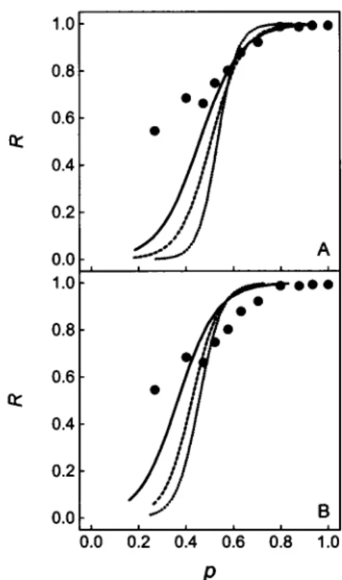
FIGURE 4 Simulation of the fluorescence fractional recovery plots ob-tained for the fixed-ellipse model for different geometries of the solid

ellipticaldomains, demonstrating the sensitivity of the result on the values of theparameters. (A)Threeoutputsfrom the fractional recovery

simula-tions,where theellipse's bla is equal to 0.2 and the semi-major axisa

equals 0.25,um(dotted line), 0.5 ,um (dashed line), and 1.0

,Am

(solidline). (B) SameasA, but with bla equalto0.3. Simulation conditions: FRAP spot radius of 3 ,um, matrix resolution r= 16points/,lm, and bilayer plane dimension6 times the spot diameter. The circles represent the experimental values.

Time-dependent recovery simulations

We shall now consider our Monte Carlo simulations of experimental FRAP curves in the timeregime for the sys-tem under examination. For these simulations we have

assumed the solid-domain topology inferred from the

former collection of simulations as apoint ofdeparture.

Thefitstothefractionalrecovery,made in theconditions

asdescribedin theMethods section,forellipseswitha = 1 ,um andbla = 0.2, aredefinitely not acceptable, as shown on Fig. 6 (series of curves numbered 2). Poor fits are

observed forfluid areafractions bothaboveand below the systempercolation threshold, which, according to Xia and

Thorpe (1988) for anaspect ratio of0.2, is 0.54. Keeping

the semi-major axis size unchanged but increasing the

as-pectratio to0.3 results inamuchbetter fit. As canalso be seeninFig. 6 (series of curves numbered 1),the model fits to the experimental dataarereasonably good for the

inter-mediate range of fluid fractions (p = 0.80-0.47). The

correspondence between the experimental and simulated

curvesbecomesquiteunacceptablefor smallfluidfractions, particularlybelow thepercolationthreshold.Therefore,

ac-cording to thesetime-resolved simulations, the best model fit leads toellipseswith an aspectratio of 0.3 andnot0.2,

asdeducedfrom the fractional recoveryatinfinitetime(see Fig. 4), for the same semi-major axis size of 1

,Am.

We shouldpointout,however,thatevenwith anaspectratioof

0.3, comparison of the simulated curves with the

experi-mental ones shows significant mismatches, particularly in theinitial phase (see, forexample, Fig. 6, C and D).

Simulations werealsoperformed forseveral other

geom-etries,witharangingfrom 0.5 to1.5 ,um, andbla from 0.2

to0.4(results notshown),but all valuesdifferentfroma = 1.0 ± 0.1

,tm

and alb = 0.3 ± 0.02 led to a worst

description ofthe experimental data.

An attempt was made to make the model morerealistic,

being fully aware that several scenarios are possible, to obtainanevenbettercorrespondencebetween the simulated andexperimentalcurves. Onesuch scenariocouldstartwith

randomly dispersed and oriented crystallization seeds and allow thesolid domainstogrow inthedirection ofboth axes

at arateinversely proportionaltothelineardimension ofthe axisperpendiculartothegrowing direction. Although more

complicated, this new growing ellipses model complies with thecrystal growththeories(Markov, 1995) and is more consistent with what is observed in macroscopic systems. Moreover, because we allow the ellipses to superpose each

other, from the diffusion point of view a dendritic-like

structure will be obtained.

Two unknownvariables are associated with the growing

ellipses model: the number of ellipses that should be

con-sidered, andtheir initial geometry. Taking into account the

fixed-ellipse geometry model fits, we postulated that at a

fluidareafraction of p = 0.52weshould have the ellipses' number and geometry given by that model, i.e., ellipses with

a = 1

,um

and bla = 0.3, ellipse density of 0.68 ellipses/ 2

_Lam,

and

positioning

in the

bilayer plane given by

the

,e 0 . A -000 , 0 0 B 1507 Coelhoetal.

A

B

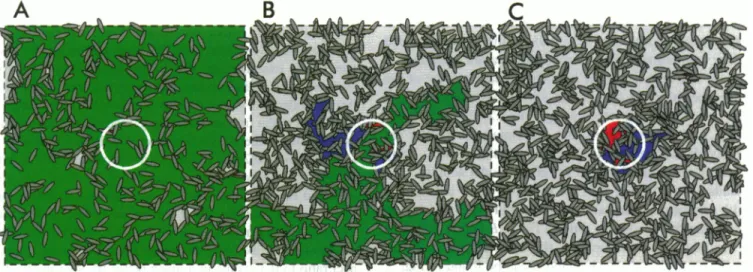
FIGURE 5 Single bilayer plane according to the fixed-ellipse geometry model for three different fluid area fractions: above (A), at (B), and below (C) the theoreticalpercolation threshold for the system, p =0.63, 0.47, and 0.40, respectively. The solid domain units are represented by ellipses with a=

1.0 ,um andb/a=0.3;the spot radius, represented by the centered circle, is 3 ,um; the matrix resolution r= 16points/,um; and the side of the bilayer plane represented is 5 times the spot diameter. In all three figures the green area represents an "infinite" fluid domain that expands outside the simulation plane, theblueareasrepresent partiallyrecoverable domains, and those painted red are totally unrecoverable domains that are inside the bleached circle. In this specific plane the fractional fluorescence recovery at equilibrium is 0.97 for A, 0.80 for B, and 0.40 for C.

simulation performed for that fluid area fraction. Although anyotherfluid area fraction could be chosen, we opted for p =0.52, becausewithin allfractions studiedit was the one

that led to the best fixed-ellipse model fit.

Afterfixing the gel characteristics for a given fluid area

fraction, we attempted by trial and error to find out the constantratio between the twoellipse axial growthratesthat would lead to the best fit through the whole set of fluid

fractions for which experimental data were available. The best result was obtained when the rate of growth in the

direction of the ellipseminor axis was90% of that for the

major axis. Under this condition the growing ellipses be-come progressively thinner, beginning with a = 0.42 and

bla=0.43, forp =0.80,andending,forp=0.40,witha= 1.29 and b/a = 0.25.

Thesimulation outputs from the ellipse growing model, together with the correlated experimental results, are pre-sented in Fig. 7. We nowobserve that the initial recovery,

dominatedby the diffusion ofprobes inthe vicinity ofthe spot,isbettersimulated, but forlongtimes there isnoreal improvement. For low fluidareafractions thedisagreement

betweenexperimentand modelcontinuestobe significant.

Fluid-domain characterization

As a result of the random placementof the elliptical solid

domains,theresultingfluid domains willobviouslyhavean

undefinedgeometry. Eventhoughwecouldnotcharacterize the fluid domains in terms of their geometry, we tried to

describe them with respect to their mean size and size

distribution. Using thesame fractional recovery simulation

applied to the fluid fractions of interest, it is possible to

make therequired calculations. Itonlymakessense tothink about finitefluid-domainsizes if the system fluidfractionis

below thepercolation threshold(p <p),because above it there will always be at least one infinite fluid cluster.

Consideringthefixed-ellipsegeometrymodel anditsbest fit to theDMPC/DSPC (1:1) system, a = 1 ,um and bla = 0.3, we present in Fig. 8 the fluid domain histograms for four different fluidfractions,oneabove and three below the system percolation threshold

(p,

= 0.46). In each plotwe

present ahistogram ofthefractional total fluid area occu-pied by domainsas afunction of their size. The histograms include all domains found.

Above, but near, the percolation threshold, atp = 0.50, althoughthemajority ofthedomainsarealreadyverysmall

(datanotshown),thegreatestcontribution tothetotal fluid

area is from very large fluid domains, where at least one

should bea"infinite" cluster.Inthiscaseperhapsit doesnot

makesense toretrievea meanfluid domain area, because it will be strongly affected by domains that arenotfinite (in realitythey are, but this is due, of course, tothe finite size

ofthe simulationplane).

Below, but still near, thepercolation threshold, thefluid domain population is now more evenly distributed, and

although infinite domains do not exist, we still have very

largefinite domains. Forafluidareafraction

equal

to

0.40,

the meanfluid domain area obtainedwas 76

,um2.

As the fluid area fraction isdecreased, the size distribu-tions of the fluid domains are

progressively

compressed

toward smaller domainareas. Themeanfluiddomain areas calculated for the fluid fractions of0.30 and 0.20were 10

,um2

and 2.5

gMm2,

respectively.

DISCUSSION

As shown in the last section, the Monte Carlo simulations

Topology ofPhase-Separated Bilayers

time

(s)

_time

_(s)

FIGURE 6 Time-dependent experimental fluorescence recovery curves obtained for theDMPC/DSPC(50/50)system (Vaz et al., 1989) for fluid

areafractions, p= 1.00, 0.80, 0.70, 0.63, 0.58, 0.52, 0.47, and 0.40. The correlative recoverycurves werecalculated fromMonteCarlo simulations considering the gel phase modeled by the fixed-ellipse model with a equal

to 1.0 ,um and two different values ofbla, 0.3 (solid line, 1) and 0.2 (dashed line, 2),correspondingtopc =0.54 andpc= 0.46, respectively.

All simulations werecarried outforaspot radius of 3 ,um, and with a

matrixresolution ofr= 16points/,um,abilayer plane dimension of 6 times the spotdiameter, and average for 1000tracermolecules perlayer in 30 simulationlayers.

different ellipse geometries, although the same topological gelmodel is used in both simulations.Furthermore,

discrep-ancies with the results and methods of other authorsmustbe

analyzed.

If, according to the fixed-ellipse geometry model, the ellipse aspect ratio should effectively be 0.3, and not 0.2, why then the bad correlation between theory and

experi-ment shown for the fractional recovery versus fluid area

(Fig. 4 B)? Theanswer tothisquestionis twofold. First, the fractional recovery deduced from the experimental FRAP

curves in cases where a significant amount of solidphase

existsareprobablynotsimplydescribablebythe Axelrodet

al. (1976)/Soumpasis (1983) expressions. The analysis of these curves force-fitted the experimental fluorescence

re-coveryprocessto a

biphasic expression

thatassumeda

rapid

diffusional process

superimposed

upon a much slower

re-coveryprocess thatwas simulated

by

alinear ramp

(Vaz

et

FIGURE 7 Time-dependent experimental fluorescence recovery curves obtained for the DMPC/DSPC(50/50) system (Vaz et al., 1989)atdifferent fluidareafractions, and thecorrespondingones asaresult ofMonteCarlo simulations.Themodel usedassumesthat thegel phase isconstitutedby

a fixed number of growing ellipses (see text for details). The ellipse geometry,indicatedbelow,wascomputed taking intoaccount a constant

ratio of axis growth rates, Vb/Va, of 0.9. The fluid area fractions and solid-ellipsegeometries represented are:p= 1.00; p = 0.80 wherea =

0.42 andbla= 0.43; p = 0.70 wherea=0.65 andb/a=0.39; p = 0.63 wherea=0.77 and bla = 0.36; p=0.58where a=0.88 and bla = 0.33;

p=0.52 wherea= 1.0andbla=0.3; p=0.47 wherea= 1.12 andbla=

0.27;andp=0.40 wherea= 1.29 andbla=0.25.Inall simulations the spotradius is 3 ,um, the matrix resolutionr= 16points/,um,and the side of theplane is 6 times the spot diameter, withanaverage of1000tracer

moleculesperlayer and 30 simulationlayers.

al., 1989).The slowregime is due in facttodiffusion with

percolationand diffusion of the tracerin gel-phasedefects,

and thereisnoway,fromasimplecurve-fittinganalysis,to

separate these two components. As shown by Saxton

(1994), the global diffusion coefficient for diffusion with

percolation is time dependent. In the limit of very short

times, the diffusion coefficient obtained tends to the

time-independent diffusion coefficient observed in a pure fluid

phase. Thus the experimental curves contain, in

fact,

two

types ofdiffusion processes thatare

physically

distinct from eachother,namely,diffusion with

percolation

anddiffusion

in gel-phase defects. The analysis of the experimental

curves, therefore, produces an artificiallyreduced value of

T

I

01) L-(a 0 0 c 0 C.) (a A B 0.8- /I. 0.6/ 0.4-0.2 -/7/ 0 0.8 C D 0.6- 0.4-0.2 ,,~

0.c1

l. r --p9. O CN 0 CN 0 0 0 0 N4 0 C') 0 C'J 04 ON 0 ) 6 A c')N d 0 -cu 0 0rea m

Fluid domainarea(tiM2)

CE) 0 CN C. '- C') C' C| CO A

N O A C'

FIGURE 8 Fluid domainhistogramscharacterizing the fixed-ellipse ge-ometry modelwithaequalto 1.0,um, blaequalto0.3 for fourdifferent fluidfractions, p=0.50(plot A), p=0.40(plot B), p=0.30(plot C),and p = 0.20(plot D).Thehistogramsrepresent thefraction ofthe total area

ofthe simulatedplaneoccupied by fluid domainsas afunction ofthe area

ofthe individual fluid domains. The labels of thexaxis, presented ina

logaritmicprogression,representtherangeof domainareascorresponding

toeachcolumn. HistogramA shows thatpractically all of the fluid in a

membranewith p = 0.50 isin continuousdomainslarger than 320 jim2 (domainscannotbelarger than the fluidareaof the simulatedplane, 648

jim2),whereasatp=0.20(histogram D),mostof the fluid isdispersed in

domains smallerthan 10jim2(totalfluidareaperlayeris259jim2).For thecalculations, squareplaneswith sides of36,um and a matrix resolution r= 16points/jumwereused. Themeanfluiddomainareasretrieved from thedistributions shownwere577jum2forp =0.50, 76jim2 forp =0.40, 10j.m2for p= 0.30,and2.5jum2forp = 0.20.

F(oo). Second, in the Monte-Carlo simulations in the time

regime we are simulating real experimental data and not conclusions derived from them. In this process the Monte Carlo methodexclusively simulates the diffusion with per-colation, no other assumptions being made.

Neither the fixed-ellipse geometry nor the

growing-ellipsemodelgivesgoodfitstothetime-dependentrecovery datafor low fluid area fractions. The initial recovery is well simulated, but for longer times, the experimentally observed recovery is much larger than the simulated one. Because DMPC (and, in particular, DMPC/DSPC (1:1)) mixtures show alargerecovery in the pure gel phase, one can be led

to thinkthat the channels in the gel, because of crystalline structural mismatch (grain boundary defects), are so large that some of therecoveries seen in cases with low fluid area fractions are due to gel-phase diffusion. This fact would

explainthelarge recoveries experimentally verified at long times. However, that cannot be the case, because the fluo-rescent probe used in the FRAP experiments partitions almost exclusively in the fluid phase, as demonstrated by fluorescence polarization (Vaz et al., 1989), and,

conse-quently,evenforvery small fluid fractions, practically all of the observed probe is actually in a fluid environment. Thus

we should seek another interpretation for the results ob-tained. Initially the fluorescence is recovered because of the diffusion of the probes present in fluid domains that are only

partially bleached. Obviously our model accounts for this phenomenon, and the initial part of thecurveis well simu-lated. Because the area of these domains is relativelysmall, their depletion is fast and the probe concentration rapidly becomes uniform. Afterward, probes from adjacent fluid pools aredrained through the channels existing in the lines ofconnection between crystals. As we have already seen, there is a significant mismatch at the grain boundaries of these crystals, and very short channels created by tangent crystals, nonpermeable to the probe in the computation, may be quite easily bridged in the real membrane. The charac-teristic time constant for thisprocess must be on the orderof magnitude of those obtained for the gel-phase diffusion. Obviously this could also be simulated, but given the

un-knowns involved, the parameters obtained would hardly have any physical meaning. The most effective way to corroborate this explanation is to make a similar Monte Carlo analysis in a experimental system in which defect diffusion between the solid domains is not significant. Pre-liminary results with the LigGalCer/DPPC (1:4) system (Almeida et al., 1992b), where diffusion in thegel phase is much less pronounced, gives support to this interpretation. To further confirm the legitimacy of our topological approach, the next obvious step would be toverify experi-mentally that the FRAP results for systems with phase coexistence are stronglydependent on the value of the spot radius, as our present results suggest. As an example, we

present in Fig. 9 two time-dependent recovery simulations brought about in the same system with the fixed-ellipse geometrymodel,but withdifferent spot radii. Asintuitively expected, the recovery obtained with a smaller area of observation (spot radius equal to 1.5 ,um) leads to a faster and more complete recovery. This evidence could be a valuable support of thephase models assumed, but again a systemhavingnegligible recovery in the gel phase would be more adequate.

In a recent paperSchram et al. (1994) studied the con-sequences of the presence ofnonoverlapping circular

obsta-0 I- U-I.U 0.86 0.4 0.2 nII 0.vO 10 time(s) 20 30

FIGURE 9 Comparisonof thetime-dependent recovery for two different FRAPspot radii. Thedashed line is obtained inthe sameconditionsas in

plot F ofFig. 6, that is, with a spot radius of 3 jum, whereas the

fluorescencerecoveryrepresented bythe solid linewassimulated forthe samebilayer topology, but withaspotof 1.5 ,um.

Coelho etal. Topology ofPhase-Separated Bilayers 1511

cles in the membrane byMonte Carlo simulation of FRAP

experiments. Their results clash with ours, because in our

case we confirm both from experiment and simulation the predictionsof the percolationtheory (StaufferandAharony,

1994; Saxton, 1994), namely, that the diffusion coefficient in a percolatingtwo-dimensional system is timedependent,

and we are led to conclude that either because of lack of resolution of the simulations performed or because the obstacles in their experimental systems are not allowed to

overlap, theywere notstudying apercolating system in the sense that we use the term here.

Using IR spectroscopy, Mendelson et al.(1995) detected domains of one to 100 molecules, the maximum domain size detectable with the techniqueused.

The dimensions of the fluid clusters estimated by San-karam et al. (1992) are much smaller (-5 orders of mag-nitude smaller) than those obtained from FRAP simulations and seeminconsistent with these. We suggest that the size of fluid domains proposed by these authors is somehow limited by the technique used. Infact, if the fluid domains in the DMPC/DSPC (1:1) system studied by these authors indeed had dimensions ofjust 100

nm2,

the fluorescence

recovery in the FRAP curves should havedroppedabruptly

at the percolation threshold (Almeida, 1992), which was

clearly not the case (Vaz et al., 1989; Vaz et al., 1990;

Bultmann et al., 1991; Almeidaetal., 1992a,b, 1993).

Thisworkwassupportedby JNICTcontractPBIC/CEN/1088/92. FPC is indebtedtoJNICT-Portugal forgrantBD/349/93.

REFERENCES

Almeida,P. F. F.1992. Lateral diffusion andpercolation in two-phaselipid bilayers. Ph.D. thesis. UniversityofVirginia. 54-71.

Almeida, P. F. F., W. L. C. Vaz, and T. E. Thompson. 1992a. Lateral

diffusion intheliquid phases of DMPC/cholesterollipid bilayers:afree volume analysis.Biochemistry. 31:6739-6747.

Almeida, P. F. F.,W. L. C. Vaz, and T. E. Thompson. 1992b. Lateral

diffusion and percolationin two-phase two-component lipid bilayers. Topology ofthe solid phase domains in plane and across the lipid bilayer. Biochemistry. 31:7198-7210.

Almeida, P. F.F., W.L. C.Vaz, and T. E.Thompson. 1993. Percolation

anddiffusioninthree-component lipid bilayers: effect ofcholesterol on anequimolar mixture oftwophosphocholines.Biophys. J.64:399-412. Axelrod, D.,D. E.Koppel,J.Schlessinger,E.Elson,W.W. Webb.1976. Mobility measurement by analysis offluorescencephotobleaching re-coverykinetics.Biophys.J. 16:1055-1069.

Bultmann, T., W. L. C. Vaz, E. C. C. Melo, R. B. Sisk, and T. E.

Thompson. 1991.Fluidphase connectivityandtranslationaldiffusionin a eutetic two-comonent, two-phase phosphatidylcholine bilayer.

Bio-chemistry. 30:5573-5579.

Derzko, Z., and K. Jacobson. 1980. Comparative lateral diffusion of

fluorescentlipid analogues inphospholipid multilayers. Biochemistry.

19:6050-6057.

Hui, S. W. 1981.Geometryofphase-separateddomains in phospholipid

bilayers by diffraction-contrast electron microscopy. Biophys. J. 34:

383-395.

Hwang, J.,L. K.Tamm, C. Bohm, T. S. Ramalingam, E. Betzig, and M. Edidin. 1995. Nanoscalecomplexity of phospholipid monolayers inves-tigated by near-field scanning optical microscopy. Science. 270:

610-614.

Keller, D.J., J. P. Korb, and H. M. McConnell. 1987. Theory of shape transitions in two-dimensional phospholipid domains. J. Phys. Chem. 91:6417-6422.

Knoll, W.,K.Ibel,and E.Sackmann. 1981.Small-angleneutronscattering study of lipid phase diagrams by the contrast variation method. Bio-chemistry. 20:6379-6383.

Luna, E.J., andH. M.McConnell. 1978.Multiple phaseequilibria in binary

mixtures ofphospholipids. Biochim.Biophys.Acta. 509:462-473. Mabrey, S., and J. M. Sturtevant. 1976.Investigationofphasetransitions

of lipids and lipid mixtures by high sensitivity differential scanning

calorimetry. Proc. Natl.Acad. Sci. USA.73:3862-3866.

Markov, I. V. 1995. Crystal growth for beginners. In Fundamentals of

Nucleation, CrystalGrowth, andEpitaxy. WorldScientific Publishing Co. Pte.,Singapore. 192.

Melo,E.C.C.,I.M.G.Lourtie,M. B.Sankaram,T. E.Thompson,and W. L.C. Vaz. 1992.Effects ofdomain connection and disconnectiononthe

yields of in-plane bimolecular reactions in membranes. Biophys. J.

63:1506-1512.

Mendelsohn, R., G.L. Liang, H. L. Strauss, andR.G.Snyder. 1995.IR

spectroscopic determination of gelstatemiscibilityinlong-chain phos-phatidylcholinemixtures.Biophys. J.69:1987-1998.

Mouritsen,0. G.,andK.J0rgensen. 1994. Dynamical orderand disorder inlipidbilayers. Chem.Phys. Lipids. 73:3-25.

Press, W.H.,B. P.Flannery, S.A.Teukolsky,and W. T.Vetterling.1989. Numerical Recipes (Fortran Version). Cambridge University Press, Cambridge.

Radmacher, M.,R. W.Tillmann, M.Fritz, and H. E. Gaub. 1992.From

moleculestocells: imaging soft sampleswith the atomic force micro-scope.Science. 257:1900-1905.

Sankaram,M.B.,D.Marsh,and T. E.Thompson. 1992.Determination of

fluidandgeldomain sizes intwo-component,two-phase bipid bilayers.

An electronspin resonance spin labelstudy. Biophys.J. 63:340-349.

Saxton, M. J. 1987. Lateral diffusion in an archipelago. The effect of

mobileobstacles.Biophys. J. 52:989-997.

Saxton, M. J. 1989. Lateraldiffusion in anarchipelago. Biophys. J. 56: 615-622.

Saxton,M. J. 1994. Anomalous diffusion duetoobstacles:aMonteCarlo study. Biophys. J. 66:394-401.

Schram, V., J.F.Tocanne, andA.Lopez. 1994. Influence ofobstacles on

lipid lateral diffusion: computersimulation ofFRAPexperiments and aplicationtoproteoliposomesandbiomembranes. Eur.Biophys.J. 23:

337-348.

Shimshick,E.J.,andH. M. McConnell. 1973.Lateralphase separationin

phospholipidmembranes. Biochemistry. 12:2351-2360.

Snyder, R. G., H. L. Strauss, and D. A. Cates. 1995. Detection and measurement ofmicroaggregation inbinary mixtures ofesters and of phospholipid dispersions.J. Phys. Chem. 99:8432-8439.

Soumpasis,D. M. 1983.Theoreticalanalysisoffluorescence photobleach-ingrecoveryexperiments.Biophys. J. 41:95-97.

Stauffer, D., and A.Aharony. 1994. Introduction to PercolationTheory. TaylorandFrancis,London.

Vaz,W.L.C. 1992.Translationaldiffusioninphase separated lipid bilayer

membranes. Comm.Mol. Cell. Biophys. 8:17-36.

Vaz,W. L.C. 1996. Consequencesof phase separations in membranes. In

Handbook of Non-Medical Applications of Liposomes, Vol. 2. Y.

Barenholz andD. D.Lasic,editors. CRCPress,Boca Raton, FL. 51-60.

Vaz,W. L.C.,and P. F. F.Almeida. 1993.Phasetopology and percolation in multi-phase lipid bilayer membranes:is thebiological membrane a domainmosaic?Curr.Opin. Struct. Biol. 3:482-488.

Vaz, W. L. C.,E. C. C.Melo, and T. E. Thompson. 1989. Translational

diffusionandfluiddomainconnectivity in a two component, two-phase

phospholipid bilayer. Biophys. J. 56:869-876.

Vaz, W. L. C., E. C. C. Melo, and T. E. Thompson. 1990. Fluid phase

connectivityin anisomorphous, two-component, two-phase

phosphati-dylcholine bilayer.Biophys. J. 58:273-275.

Wiener, M. C., R. M. Suter, and J. Nagle. 1989. Structure of the fully

hydratedgel phase ofdipalmitoylphosphatidylcholine. Biophys. J. 55:

315-325.

Wu,S.H.,and H. M.McConnell. 1975.Phase separation inphospholipid

membranes.Biochemistry. 14:847-854.

Xia, W., and M. F. Thorpe. 1988. Percolation properties of random ellipses. Phys. Rev. A. 38:2650-2656.