Unusual Domain Growth Behavior in the Compressible Ising Model
S. J. Mitchell,∗ Luiz F. C. Pereira,† and D. P. Landau‡ The Center for Simulational Physics, and the Department of Physics,
University of Georgia, Athens, GA 30602-2451, USA
Received on 28 August, 2007
Large scale Monte Carlo simulations have been used to study long-time domain growth behavior in a com-pressible, two-dimensional Ising model undergoing phase separation. The system is quenched below the transition temperature from a random spin state, and we investigated the late-time domain size growth law, R(t) =A+Btn. For “lattice mismatched” systems, we foundn=0.224±0.004 which deviates significantly from the Lifshitz-Slyozov value ofn=1/3 for late-time growth . For a compressible model with no mismatch, we find only a slight deviation fromn=1/3. These results strongly suggest that we do not yet fully understand domain growth.
Keywords: Ising Model; Compressible Model; Phase Separation; Domain Growth
I. INTRODUCTION
The phenomenon of phase separation is extremely common in diverse condensed matter systems including magnets [1, 2], alloys [3–14], fluids [15–20], and polymers [21]. Phase sepa-ration may be observed whenever a system is quenched from a homogeneous disordered phase into an ordered phase where multiple domains coexist. During phase separation, diffusion and surface tension cause the domain size to increase with time. For an infinite system, the domain size is predicted to grow as a power law [22],
R(t) =A+Btn, (1)
whereRis the domain size,tis the time after the quench oc-curs,AandBare constants which depend upon system spe-cific details, and nis the domain growth exponent [1]. Sto-chastic domain growth with a conserved order parameter in the absence of hydrodynamic modes (Model B [23]) is be-lieved to be in a class of domain growth with n=1/3, in-dependent of the dimensionality of the system. This value for the growth exponent, first predicted by Lifshitz and Sly-ozov [24], has since been observed in numerous simulation results of lattice models, most notably Ref. [1]. For reviews, see Refs. [25–27]. Thus, it would seem as though domain growth under these conditions would not show the rich diver-sity of behavior that is seen near critical points in different systems.
Monte Carlo simulations are well suited for the study of do-main growth under these conditions, but because large system sizes are required to access the asymptotic growth limit region and multiple long runs are needed to measuren, few high pre-cision computational studies exist that could verify the univer-sality of then=1/3 growth law. Furthermore, until recently, high precision studies of compressible systems were outside the limits of available computational resources. Studies of
∗Electronic address:steven.mitchell2@bp.com †Electronic address:pereira@physast.uga.edu ‡Electronic address:dlandau@hal.physast.uga.edu
Ising binary alloys [28–32] have now shown that compress-ibility can affect static critical phenomena and can have a non-trivial effect on the interfaces between domains [17]. There is reason to believe that domain growth may also be affected by compressibility [4, 6]; however, we are unaware of any high precision computational study that has confirmed any signifi-cant deviation from the theoretical prediction ofn=1/3.
II. MODEL AND METHOD
In order to investigate the universality of the n =1/3 growth law, we have considered the simplest possible com-pressible model with coherent interfaces, a two-dimensional Ising model in which L2 Ising spins have continuous posi-tions within a periodic box of sizeLx×Ly. Although the Ising model is most often used to describe magnetic systems, it is equivalent to a binary alloy in which the two spin values rep-resent the two different species. The Ising model Hamiltonian is
H
=∑
i j
f(ri j,si,sj) +Jθ
∑
i jkcos2(θi jk), (2)
where∑i jis a sum over nearest-neighbor pairs of particles, ri j is the distance in dimensionless units between nearest-neighbor particles, si is the spin value of the ith spin with possible values of ±1, f(r,a,b) is the nearest-neighbor in-teraction potential (given below),Jθ=50 is the bond angle stiffness in dimensionless units, and ∑i jk is the sum over bond anglesθi jk(four per particle), whereiandkare nearest-neighbors of j. The second term stabilizes an ordered square lattice structure.
In this model the nearest-neighbor interaction is given by a Lennard-Jones-like potential:
f(r,a,b) =Jab
lab r
12
−2
l
ab r
6
, (3)
10 MCS
4
10 MCS
5
10 MCS
6
rigid 0% mismatch 4% mismatch
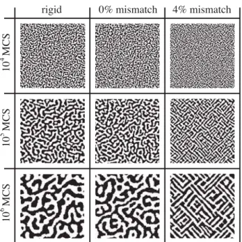
FIG. 1: Configurations at different times for each model. L=512. Down spins (−1) are white, and up spins (+1) are black. The tem-perature is 0.59Tcfor the rigid model, and is close to 0.6Tc(T=1.5) for the compressible models.
With these interactions, when lab=1 and J++ andJθ→∞, the Hamiltonian reduces to that of the common ferromagnetic, rigid (lattice) Ising model, allowing comparison with previous studies [1]. We will give all spatial units in terms of thel+− bond length, and all energies and temperatures in units where J++−J+−=2. The well-known Onsager critical temperature for the rigid (lattice) model is thusTc=2.269.
The model was investigated using Monte Carlo simulations with the standard Metropolis acceptance criterion within the canonical constant pressure ensemble [33]. Three types of Monte Carlo moves were used: a spin exchange (Kawasaki dynamic), in which a nearest neighbor pair of spins were ran-domly chosen and their spin values exchanged, lateral dis-placement, in which a particle was randomly selected and its position displaced by a small, random amount, and a global volume rescale (expansion or contraction), which was needed to maintain a constant pressure. The energy change for the global rescale had an additional effective term not shown in Eq. 2, which was needed to correctly reproduce a constant pressure ensemble [28]. Monte Carlo time was measured in units of Monte Carlo steps per site (MCS), where one MCS consisted of one attempted volume change followed byL2 ex-change or lateral displacement attempts, where the probability to choose exchange or displacement was 50%. For the rigid (lattice) model, only spin exchange moves could be imple-mented, and then one MCS consisted ofL2exchange attempts. Each simulation began with a state in which the value of each spin was randomly chosen to be +1 or−1 with 50% probability, and our Monte Carlo algorithm conserved the to-tal magnetization at this initial value. The system was then equilibrated at a temperature (T =7.0) which was well above
0 20 40 60
r -0.2
0 0.5 0.5 1
C(r)
103 MCS
106 MCS
0% mismatch
FIG. 2:C(r)for the 0% mismatch model at various times.L=512, averaged over the lattice and lattice diagonal directions for 56 runs. (For the rigid and 0% mismatch models,C(r)is isotropic.) Error bars are less than the line thickness.
the critical temperature (Tc). Following equilibration the tem-perature was quenched to 0.6Tc, and the configurations were recorded and analyzed every 103MCS.
III. RESULTS
We investigated three specific variations of the model, the rigid two-dimensional Ising model (i.e. the traditional Ising square lattice), a symmetric elastic net, where lab=1, re-ferred to as the 0% mismatch model, and a 4% lattice mis-match model, where l++=1.02 and l−−=0.98. The 4% mismatch value was chosen to give insight into phase separa-tion in SiGe alloys [28–30]. To decrease the computasepara-tional ef-fort of the simulations, the compressible systems were treated as distortable square nets, a reasonable approach for the low temperatures and relatively stiff models considered here.
All simulations were performed in the spinodal decompo-sition regime, as the configurations in Fig. 1 indicate, and all three variations of the model clearly show phase separation behavior [34]. No noticeable qualitative differences in the overall structure can be seen in the “snapshots” of the rigid and 0% mismatch models; however, the 4% mismatch model shows clear, diagonally oriented domains. Anisotropic con-figurations are often observed for systems containing a lattice mismatch [10]. A system with coherent interfaces, such as the one studied here, might be expected to stop phase separating at very late times (not reached in these simulations) [14], where the domain size would be finite due to interfacial energy.
Simulations were performed for various system sizes be-tweenL=64 andL=512. These showed that system sizes ofL=512 (5122 particles)and time scales of 106MCS are
0 1 2 3 4
r/
ξ
-0.2 0 0.5 0.5 1
C(r/
ξ
)
103 MCS 104 MCS
105 MCS
106 MCS 0% mismatch
FIG. 3:C(r/ξ)vs “scaled distance”r/ξfor the 0% mismatch model at various times. The data are forL=512, from Fig. 2.
0 20 40 60
r -0.5
0 0.5 1
C(r)
103 MCS 106
MCS 3x10⁴ MCS
4% mismatch
FIG. 4:C(r)for the 4% mismatch model at various times.L=512, averaged over the lattice directions for 69 runs. (For the 4% mis-match model,C(r)is anisotropic, with no zero crossing in the diag-onal directions at late times.) Error bars are less than the line thick-ness.
time series. The rigid model (lattice) simulations accounted for less than 5% of the total computational effort and are in-cluded for comparison to earlier work [1] that used a vector-ized, multispin coding algorithm. Although we would not ex-pect any difference inn, the vectorizing algorithm examined the spins in a different order and could yield different values ofAandB. Note that larger system sizes and longer runs are not feasible for the compressible models with currently avail-able resources, sinceL=1024 only reaches 105 MCS after two weeks of run time. On the other hand, simulations for L=256 show finite size effects fort∼107 MCS so longer simulations would not help for this size system.
Quantitative information about the phase separation behav-ior can be extracted by analyzing the spin-spin spatial cor-relation function; however, because the compressible mod-els have continuous particle positions, methods developed for regularly spaced particles were not applicable. Therefore, the correlation function was calculated by direct summation over
0 1 2 3 4 5 6 7
r/
ξ
-0.5 0 0.5 1
C(r/
ξ
)
3x10⁴ MCS 103 MCS
104 MCS
105 MCS
3x10⁵ MCS
106 MCS 3x10³ MCS
4% mismatch
FIG. 5:C(r/ξ)for the 4% mismatch model at various times. Data are forL=512, from Fig. 4.
the “lattice” in only four “high symmetry” directions,
C(r) =C(p,q)(r) =sisj, (4) where(p,q)denotes one of the four displacement directions, i.e. the “lattice” directions,(1,0)and(0,1), and the “lattice” diagonal directions, (1,1) and(−1,1). Furthermore, si and sj are the spin values of two particles with a displacementr in the(p,q)direction, andsisjdenotes an average over all such pairs of particles. For brevity,ris used here to denote an average over the actual interparticle displacements. The correlation length,ξ, is then defined as the first zero crossing ofC(r)and is found by fitting a second order polynomial to the three points closest to the crossing.
The correlation functions were isotropic for both the rigid (lattice) model and the 0% mismatch model, and Fig. 2 shows C(r)averaged over all four directions for 0% mismatch. Both the rigid and 0% mismatch models show well-defined first zero crossings for all directions, and the zero crossing moves to greater distances as the time increases. When the correla-tion funccorrela-tion is plotted against the “scaled” correlacorrela-tion length, see Fig. 3, the curves almost collapse onto each other. In contrast, with 4% mismatch we find quite anisotropic results, as one might expect from Fig. 1. For the (1,0)and (0,1)
directions, see Fig. 4 the first zero crossings again move to greater distances with increasing time, moreover, additional zero crossings are visible on this scale. Fort>104MCS, no first zero crossing is observed in the diagonal directions, but we can perform alternative scaling analyses using the loca-tion of the first local minimum or the perimeter density (i.e. fraction of mixed bonds). These additional analyses yielded the same growth exponents as those obtained from the first-zero crossings presented below. When the correlation function is plotted against the “scaled” correlation length, see Fig. 5, the curves do not collapse onto each other, although the zero crossings occur quite close to each other.
non-103 104 105 106
t [MCS]
1 3 10 30
ξ
-A
ξ=A+Btn, fit for t>104 MCS rigid, 256 runs
0% mismatch, 56 runs 4% mismatch, 69 runs
FIG. 6: Time dependence ofξ(t)−AforL=512. Lines are least squares fits to A+Btn, wheren is the domain growth exponent. Data were averaged over multiple runs and directions. Error bars are smaller than the symbol sizes.
104 105 106
t [MCS]
0.20 0.25 0.30 0.35
n
n=0.224 n=1/3
rigid
0% mismatch
4% mismatch
FIG. 7: Results of the ratio analysis forL=512,∆=4×10³MCS, bin averaged over eight points (original point separation 103MCS). While error bars are not shown, statistical errors can be estimated from the fluctuations of the results.
linear fits to the data shown in Fig. 6 fort >104, we find
thatn=0.332±0.003 for the rigid model,n=0.318±0.005 for the 0% mismatch model, and n=0.224±0.004 for the 4% mismatch model. The error bars include small systematic uncertainties arising from the fitting procedure, such as the number of points, weighting of the data, and fitting range.
In addition to performing least squares fits of the long time behavior of the domain size, shown in Fig. 6, we also per-formed a ratio analysis [33], which is a more sensitive tech-nique giving a “local” estimate of the growth exponent, i.e. over a relatively short time interval. The ratio estimate for n(t)is defined by
n(t) =log
ξ′(t+∆)
ξ′(t−∆)
logt+∆ t−∆
, (5)
whereξ′(t) =ξ(t)−A,Ais obtained from fits shown in Fig. 6,
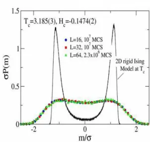
FIG. 8: Plot of the scaled magnetization distribution vs scaled mag-netization for 4% mismatch compressible systems at the estimated location of the critical point (see the top of the figure). Errors are smaller than the size of the symbols.
andt and ∆ are multiples of 103 MCS. Because the ratio method is very sensitive to small statistical errors inξ(t), bin averaging of the final sequence was necessary. Therefore, the calculation was repeated for different bin widths and different values of∆andA, but such differences did not noticeably af-fect the estimate ofn. The results from the ratio analysis are shown in Fig. 7.
The growth exponent estimates for the lattice (the rigid model) are in excellent agreement with the theoretical pre-diction ofn=1/3 [1, 23–25, 33]. The small deviation from n=1/3 for 0% mismatch is within the fluctuation in the “lo-cal estimates” forn; hence we cannot firmly conclude that it is inconsistent withn=1/3 at long times. Longer runs and larger systems would be needed to determine if this deviation is a real effect, but such simulations are beyond our current computational capabilities. However, for the 4% mismatch model the results clearly show a smaller growth exponent and anisotropic correlations. (Deviations fromn=1/3 have been seen before in systems with mismatch [4], but it was unclear if the asymptotic growth regime had been reached, and more recent studies [9] indicatedn=1/3.)
which is included in the figure for comparison. Note that field mixing was not employed, and it is possible that an even bet-ter scaling could be obtained if it were implemented; but even without field scaling the data scale extremely well.
The “universal” curve expected for systems in the same uni-versality class as the two dimensional Ising model is dramat-ically different and strongly suggests that the compressible, Ising net is not in the same static universality class as the Ising lattice model.
IV. CONCLUSION
The inclusion of compressibility and lattice mismatch in the Ising model Hamiltonian can alter the domain growth
ex-ponent, and our results can be readily generalized to systems with differing sizes or differing bond lengths. We do not know if the deviations fromn=1/3 indicate a breakdown of univer-sality or if they indicate new classes of domain growth. Obvi-ously our current understanding of domain growth is incom-plete, and further theoretical and computational consideration is needed.
Acknowledgments
The authors thank S. H. Tsai and K. Binder for helpful com-ments and discussions. This work was funded by NSF grants #DMR-0341874 and #DMR-0307082.
[1] J. G. Amar, F. E. Sullivan, and R. D. Mountain, Phys. Rev. B 37, 196 (1988).
[2] P. Fratzl, J. L. Lebowitz, O. Penrose, and J. Amar, Phys. Rev. B 44, 4794 (1991).
[3] A. Sadiq and K. Binder, J. Stat. Phys.35, 517 (1984). [4] H. Nishimori and A. Onuki, Phys. Rev. B42, 980 (1990). [5] A. Maheshwari and A. J. Ardell, Phys. Rev. Lett. 70, 2305
(1993).
[6] C. Sagui and R. C. Desai, Phys. Rev. Lett.74, 1119 (1995). [7] C. A. Laberge, P. Fratzl, and J. L. Lebowitz, Phys. Rev. Lett.
75, 4448 (1995).
[8] V. I. Gorentsveig, P. Fratzl, and J. L. Lebowitz, Phys. Rev. B 55, 2912 (1997).
[9] P. Nielaba, P. Fratzl, and J. L. Lebowitz, J. Stat. Phys.95, 23 (1999).
[10] D. Orlikowski, C. Sagui, A. M. Somoza, and C. Roland, Phys. Rev. B62, 3160 (2000).
[11] R. Weinkamer, P. Fratzl, H. S. Gupta, O. Penrose, and J. L. Lebowitz, Phase Transitions77, 433 (2004).
[12] K. Binder and D. Stauffer, Phys. Rev. Lett.33, 1006 (1974). [13] P. Fraztl, O. Penrose, and J. L. Lebowitz, J. Stat. Phys.95, 1429
(1999).
[14] B. J. Schulz, B. D¨unweg, K. Binder, and M. M¨uller, Phys. Rev. Lett.95, 096101 (2005).
[15] T. Koga and K. Kawasaki, Physica A196, 389 (1993). [16] A. T. Bernardes, T. B. Liverpool, and D. Stauffer, Phys. Rev. E
54, R2220 (1996).
[17] S. K. Das, S. Puri, J. Horbach, and K. Binder, Phys. Rev. Lett. 96, 016107 (2006).
[18] M. Grant and K. R. Elder, Phys. Rev. Lett.82, 14 (1998). [19] V. M. Kendon, J. C. Desplat, P. Bladon, and M. E. Cates, Phys.
Rev. Lett.83, 576 (1999).
[20] P. B. Warren, Phys. Rev. Lett.87, 225702 (2001).
[21] T. Hashimoto, M. Itakura, and H. Hasegawa, J. Comp. Phys. 85, 6118 (1986).
[22] D. A. Huse, Phys. Rev. B34, 7845 (1986).
[23] P. C. Hohenberg and B. Halperin, Rev. Mod. Phys.49, 435 (1977).
[24] I. M. Lifshitz and V. V. Slyozov, J. Phys. Chem. Solids19, 35 (1961).
[25] A. J. Bray, Adv. Phys.43, 357 (1994).
[26] A. Onuki, Phase Trasition Dynamics(Cambridge University Press, Cambridge, 2002).
[27] J. D. Gunton, M. S. Miguel, and P. S. Sahni, inPhase Transi-tions and Critical Phenomena, Vol. 8, edited by C. Domb and J. L. Lebowitz (Academic Press, New York, 1983).
[28] B. D¨unweg and D. P. Landau, Phys. Rev. B48, 14182 (1993). [29] M. Laradji, D. P. Landau, and B. D ¨unweg, Phys. Rev. B51,
4894 (1995).
[30] F. Tavazza, D. P. Landau, and J. Adler, Phys. Rev. B70, 184103 (2004).
[31] D. P. Landau, F. Tavazza, and J. Adler, Comp. Phys. Commun. 169, 149 (2005).
[32] E. M. Vandeworp and K. E. Newman, Phys. Rev. B55, 14222 (1997).
[33] D. P. Landau and K. Binder,A Guide to Monte Carlo Simu-lations in Statistical Physics, 2nd ed. (Cambridge University Press, New York, 2005).