1
A Project carried out on the Macroeconomics of Financial Markets and Theory of Finance course (LUISS Guido Carli) courses (NOVA SBE), and
under the supervision of: Prof. André C. Silva (NOVA SBE) Prof. Nicola Borri (LUISS Guido Carli)
A Work Project, presented as part of the requirements for the Award of a Double Degree of Masters Degree in Financial Economics from the LUISS Guido Carli and of Masters
Degree in Finance from the NOVA – School of Business and Economics
Vasco Polónia Marques Laranjo, nº 761
June 2015
2
Abstract
This Working Project studies five portfolios of currency carry trades formed with the
G10 currencies. Performance varies among strategies and the most basic one presents
the worst results. I also study the equity and Pure FX risk factors which can explain the
portfolios’ returns. Equity factors do not explain these returns while the Pure FX do for
some of the strategies. Downside risk measures indicate the importance of using regime
indicators to avoid losses. I conclude that although using VAR and threshold regression
models with a variety of regime indicators do not allow the perception of different
regimes, with a defined exogenous threshold on real exchange rates, an indicator of
liquidity and the volatilities of the spot exchange rates it is possible to increase the
average returns and reduce drawdowns of the carry trades.
3
I. Introduction
This Working Project explores several questions related to the currency carry trade
arbitrage strategy. Firstly, it is studied whether the strategy is profitable or not,
especially, after the event of the 2008’s global financial crisis. In order to do this, five
portfolios of the G10 currencies with different weighting strategies used among
literature and by practitioners are investigated. Secondly, the latest literature emphasizes
the tail and downside risks intrinsic to the strategy and, thus, several measures of
downside risk and, specifically, a drawdown analysis is performed. At last, the final
purpose of this work is answering to the following two questions: are there any regime
indicator variables that allow to consistently predict a drawdown on the strategy? How
can an investor use these regime indicators to improve his final payoff?
To begin with, in financial terms an asset’s “carry” is equal to the returns (positive
carry) or the costs (negative) of holding such asset, assuming its price does not change.
In that sense, it is possible to break down a security’s return into three components: the
carry, its expected and unexpected price appreciation.1 Moreover, when “carry trade” is
mentioned one is referring to a strategy composed by two or more offsetting positions
on an asset’s class, where some securities are returning a positive cash-flow while
others constitute a liability. This strategy can be exploited over a variety of classes such
as global equities and bonds, Treasuries, index options, currencies and commodities.
Nevertheless, its most widespread application is on currencies, which is known as the
“currency carry trade” and it is argued to date back to the 80’s.
In the currency carry trade an investor borrows in a country with a low interest rate and
invests in another with high interest rate, gaining the carry this way. Therefore, such
1
4
strategy has been presenting high returns and long-run Sharp ratios over time, despite
recent losses. Additionally, the most puzzling question is that it is based on an
international economics’ hypothesis known as the uncovered interest rate parity (UIP)
which states that nominal interest rate differentials between countries have a direct
relationship with market’s expectations of exchange rates’ changes. That is, in
accordance with the UIP a high-yield currency should depreciate by the size of the
interest rates’ differential, thus, leading to capital losses that would fully offset the gains
from the yield advantage. In that sense, consider for instance the most popular pair for
the carry trade in recent years: the Japanese yen as funding currency and the Australian
dollar as investment currency. Let us consider that the yield in Australia was 6% higher
than in Japan in 2007, then the AUD/JPY spot exchange was expected to depreciate 6%
over the next year. However, empirical studies starting from 1980 have consistently
proven this wrong as on average the subsequent currency depreciation did not
completely offset the carry from the interest rate differential. Finally, this finding is
known as the “forward rate bias” as a result of the rejection of the expectations theory
hypothesis.
Furthermore, when undergoing a currency carry trade it is preferable to analyze
currencies exposed to a low probability of default which is a risk that an investor is
usually not willing to take in this strategy, since the only risk he accepts to face is the
exchange rate risk. Thus, since the returns for the strategies using the G10 countries
remained high until the beginning of the 2008’s global financial crisis and the default
risk is much lower than in emerging markets the general approach when studying the
currency carry trade it is preferred to use a basket of these G10 currencies. In addition,
most of the studies use a timespan starting after 1973 due to the collapse of the Bretton
5
studies have shown that by investing in this strategy an investor can obtain high average
returns ranging from 3,96% in basic strategies to 6,6% in more complex ones, when
considering a time range of 1976-2013.2 In that sense, in this Working Project it is
intended to investigate the results of several carry trade strategies and the evolution of
their performance. Additionally, it is commonly stated that the carry trade strategy was
not profitable after the 2008 financial crisis or that the strategy “is not dead but
resting”3. Taking this into consideration, attention is devoted to a comparison of the
results between the pre- and post-crisis periods.
Furthermore, after finding that UIP did not hold on average, researchers focused their
attention on the risk factors explaining the currency carry trade returns. Nevertheless,
returns from different carry trade strategies have hardly been explained by traditional
risk factors, thus, leaving the currency carry trade as a puzzle. Hence, due to the long
list of studies on these risk factors in the literature, it was preferred not to emphasize
this aspect of the carry trade presenting merely a short analysis of the latter.
Lately, recent studies have focused on an apparent downside of the strategy which is the
negative skewness inducing large drawdowns. This pattern has been named as “up by
the stairs, down by the elevator” or “picking up nickels in front of a steam roller”.4
Aiming at understanding this component of the carry trade, it was decided to dedicate
one chapter of this Working Project to the analysis of four indicators of downside risk.
In conclusion, as these large drawdowns are related to the carry crashes, its timing is
known to be the “jackpot question of the carry trade”.5 Contrary to the investigation of
2 These are the results of both the EQ and SPD weighting strategies presented in Daniel et al. (2014) 3
On the 15th of January of 2013, Jame Mackintosh wrote on Financial Times and article with the time: “Carry trade strategy not dead but resting”.
4
Expression used by Breedon (2001) and the economist in 2007, respectively. 5
6
risk factors explaining the carry trade returns, only a few studies explore the hypothesis
of using regime indicators to improve the returns of the strategy. Thus, the present
Working Project’s final purpose is to find the regime indicator variables which can used
to forecast and avoid the carry crashes and, therefore, improve the strategy’s
profitability.
The following text is organized as it follows: in chapter II a brief Literature Review is
presented, while in chapter III an explanation on the construction of the carry trade
strategies is presented. Chapter IV presents all the sources for the data used in this
Working Project and leads to chapter V where the results of the strategies are
commented. Successively, chapters VI and VII show the study of the traditional and the
downside risk factors, respectively. Finally, in chapter VIII the regime indicator
analysis is studied and in chapter IX the conclusions are displayed.
II. Literature Review
The studies on the failure of the interest rate parity hypothesis are agreed to have started
in the late 70’s ormore specifically in the 80’s with papers such as Hansen and Hodrick
(1980) where the market efficiency hypothesis for exchange rates is rejected for a
period of 50 years before the 1970’s. Also, Fama (1984) presents results where the
reverse effect expressed by the UIP is verified. Moreover, Daniel et al. (2014) explores
four different approaches on the rejection of the unbiasedness of forward rates.
Nevertheless, recent literature has focused on two of these explanations: the equilibrium
risk premium in the forecastability of the difference between forward rates and future
spot rates (e.g. Hansen and Hodrick (1983)); and in the presence of peso problems
7
Simple carry trade strategies have historically presented high average returns and
Sharpe ratios as shown in Burnside (2012). Furthermore, more complex strategies
determining the weights on a basket of currencies as studied in Daniel et al. (2014)
improve the carry trade’s performance. Other common strategy is known as
High-minus-Low where the investor holds a long position in a number of high-yield
currencies while shorting the same number of low-yield.6 Another way of applying the
latter strategy is by using portfolios of currencies instead of a single currency as it was
firstly explained in Lustig and Verdelhan (2007).
Risk explanations to the high returns fall into many categories from traditional risk
factors to the mentioned “peso problems”. The traditional risk factors usually include
the Fama and French 3-factor model (1993) as it was used in Burnside (2012) and
Daniel et al. (2014). Additionally, Lustig, Roussanov and Verdelhan (2011) use the
return on the highest minus the return on the lowest interest rate currency portfolios to
explain the cross-sectional variation in average currency excess returns from low to high
interest rate currencies. Exchange rate volatility, likewise, seems to be one of the most
important factors explaining the risk of carry trade strategies as it is argued that the
global FX volatility risk captures more than 90% of the cross-sectional excess returns in
five carry trade portfolios in Menkhoff et al. (2012). Also Christiansen, Ranaldo and
Söderlind (2011) use FX volatility to explain carry trade abnormal returns. Moreover,
another suggested risk indicator in the literature is consumption growth proposed in
Lustig and Verdelhan (2007) while using a CCAPM model. More recently Jurek and Xu
(2013) use options in the currency market to show that option-implied currency risk
premia provide an unbiased forecast of monthly currency excess returns.
8
In addition, a common global risk indicator is also popular among researchers having
been proposed by Dahlquist and Hasseltoft (2013) who used the US bond risk premia
and demonstrated it to be related to international business cycles. On the other hand,
Lustig, Roussanov and Verdelhan (2011) construct a slope “factor” in a model with a
country specific and global factors which is related to changes in the global equity
market volatility and which identifies common shocks. The equity market returns are
also a competitive risk explanation as Campbell et al. (2010) found that many
currencies in particular the Australian dollar, Canadian dollar, Japanese yen, and British
pound are positively correlated with world stock markets while the euro, the Swiss
franc, and the bilateral US-Canadian exchange rate are negatively correlated with the
world equity market. Alternatively, Corcoran (2009) demonstrate a correlation between
carry trades and target-country equity markets’ returns which is negative for high
interest rate currencies and positive for low interest rate currencies.
Finally, recent studies have focused on the “peso problems” and more specifically in the
downside risks of the carry trade. Farhi et al. (2015) argue that the carry trade is
exposed to rare crash states in which high interest rate currencies depreciate. Adding to
this, Brunnermeier et al. (2009) claim that carry traders are subject to crash risk where
exchange rate movements between high-interest-rate and low-interest-rate currencies
are negatively skewed while pointing out that this is due to sudden unwinding of carry
trades, which tend to occur in periods where risk appetite and funding liquidity
decrease. Also, Gyntelberg and Schrimpf (2011) while studying short-term
multicurrency strategies such as the carry trade demonstrate that these strategies exhibit
substantial tail risks and that they do not perform regularly during periods of financial
distress in global markets. Still, the authors find that there is an even greater downside
9
Lastly, recent work has been developed on the hedged carry trade using exchange rate
options. Burnside et al. (2011) shows in a clear way how to construct such portfolios,
however, despite obtaining a positive skew it yields much lower average returns and
Sharpe ratio. Other examples of the hedged carry trade strategy are Caballero and Doyle
(2012) who affirm that hedge carry trades with exchange rate options present large
return which are not explained by incurring in systemic risk; as well as, Jurek (2013)
where by constructing crash-hedged portfolios he shows that peso problems do not
explain carry trades’ high returns.
III. The Carry Trade portfolios implementation
In this section, the notation and theoretical background that is necessary to proceed to
the empirical analysis of the carry trades will be presented. Thereafter, it is shown the
procedures to construct the different strategies to be discussed. Let St be the level of the
exchange rate of dollars per unit of a foreign currency, while Ft. is the forward
exchange rate known today for the exchange of currencies one period-ahead. At the
same time, the one-period dollar interest rate is represented by it$ and let the one-period
foreign currency interest rate be it∗.
The carry trade involves the lending of a high-interest rate currency by borrowing a
low-interest rate currency. It follows the failure of the UIP in the sense that if the
exchange rate between two countries does not evaluate or depreciate in order to offset
the interest rate differential between the latter there will be an arbitrage opportunity.
Consider below the UIP:
UIP: (1 + it$) =E(SSt+1)
t (1 + it
10
Therefore, the typical studied strategy in the literature is the one where an investor takes
a long (short) position in each currency for which the interest rate is higher (lower) than
the interest rate in the United States. This strategy is applied when the investor borrows
or lends in the money market and, thus, the dollar payoff to the carry trade in the
absence of transaction costs is written as such:
zt+1 = [(1 + it∗)St+1
St − (1 + it$)] yt
where the position the investor takes in each currency (yt) is:
yt = {+1 if it∗ > it$ −1 if it∗ < it$
Alternatively, an investor can enter in a carry trade strategy by borrowing or investing
one dollar in the foreign currency money market. Consider that when the covered
interest rate parity holds, if it∗ > i t
$ then Ft < St, that is, the foreign currency is at a
discount in the forward market. On the other hand, if it∗ < it$ then Ft > St and, thus, the
foreign currency is at a premium in the forward market. Therefore, it is also possible to
develop a carry trade strategy by entering in a long (short) position in the forward
currency’s market when the foreign currency is at a discount (premium) in comparison
to the dollar. Finally, the dollar payoff to this strategy is as it follows:
zt+1 = [(St+1F− Ft)
t × (1 + it $)] y
t
where the position the investor takes (yt) is:
yt = {+1 if F−1 if Ftt < St> St
(4)
(5) (2)
11
It is worth to notice that when the covered interest parity holds and without transaction
costs, both strategies for the implementation of the carry trade are exactly equivalent.
The former seems to have been realized until the onset of the financial crisis in August
2007, according to Coffey et al. (2009). Although, different liquidity conditions in the
interest rates and forward exchange markets might dictate higher transaction costs. If
the uncovered interest rate parity holds and the forward rates are unbiased, the carry
trade profits should average to zero. Still, recall that the definition of the uncovered
interest rate parity ignores that the changes in the values of currencies may be exposed
to risk factors and, therefore, in this situation a risk premium is observed. Thus, the
general procedure to incorporate risk aversion in arbitrage models is to examine the
stochastic discount factor (SDF) or pricing kernels.
3.1 Stochastic Discount Factors (SDF) and the Arbitrage Asset Pricing
In order to confirm the fundamentals of no-arbitrage pricing it must be verified that
there is a dollar stochastic discount factor, Mt+1, that prices the nominal USD
denominated excess returns, Zt+1. Furthermore, since the carry trades under study are
zero-investment strategies, the no-arbitrage condition is:
Et(Mt+1× Zt+1) = 0
Recalling the covariance composition and applying it to the previous equation it is
derived:
Et(Zt+1) = −Cov(Mt+1, Zt+1)Et(Mt+1)
The analysis of the previous equation is highly important in order to study whether there
are risk factors capable of explaining the carry trades returns and, thus, producing a
12
specified. In section VI, I will present some candidate risk factors. For a longer
explanation on the SDF methodology refer to Burnside (2012), while Menkhoff et al.
(2012) develops an explanation on the econometric procedures to follow in the risk
factors’ regression.
3.2. Constructing the carry trade strategies
In this part of this study it will be presented the five carry trade portfolios with different
weighting strategies. Carry trades have been popular for a long time, which led
investors to develop different strategies on how to be exposed to each currency. This
exposition to each currency is defined by the weight that is allocated to the currency and
the most popular is the equally weighted (EW) in that the weights are equal for every
currency, where N is the number of available currencies at the period t:
wj,tEW =sign(it j − i
t $) N
However, it may be that an investor wants to take more speculative positions in each
currency at a time since the positions of the previous strategy tend to be much lower. In
order to do it he can use one carry trade strategy suggested in Daniel et al. (2014) which
the authors name as speed-weighting (SPW). The idea is that “the fraction of a dollar
invested in a particular currency is determined by the interest differential divided by the
sum of the absolute values of the interest differentials”. Therefore, this strategy
privileges currencies with larger interest rates’ differentials while at the same time
allowing the investment to be scaled such that there is one dollar spread across the long
and short positons. Therefore, the weights are as it follows:
wj,tSPW = itj − it$ ∑ |iNt tj − it$|
j=1
(8)
13
Additionally, another common strategy comes by hedging the exchange risk on the EW
strategy by acquiring (selling) forward exchange rate contracts on a currency when
entering a long (short) position on that currency, accordingly. In that sense, at t+1 the
investor is still exposed to the currency value (St+1) but now the value he holds of the
same currency is not the investment in terms of St but in Ft. Finally, it is important to
keep in mind that for the previous three strategies in a situation where the sum of the
currency weights is not equal to 0, the dollar is used to made this correction. In order to
perform such strategy I consider the same weights of EW but now the payoffs are as it
follows:
zt+1 = [(1 + it∗)SFt+1
t − (1 + it $)] y
t
A different approach which also proved to be highly profitable is suggested by Lustig,
Roussanov and Verdelhan (2014) and is called the “dollar care trade” since “investors
go long all foreign currencies when the average foreign currency trades at a forward
discount and short all foreign currencies when the average foreign currency trades is at a
forward premium.” Then, this position is balanced by the investment in the dollar by
investing in the US interest rate. Moreover and contrarily to the remaining strategies
with the intention of preserving the authors’ results equation (4) is used instead of
equation (2).
At last, Antti Ilmanen in his book “Expected Returns: An Investor's Guide to Harvesting
Market Rewards” of 2011 presents a strategy which here will name as ranking once an
investor should weight differently his positions on each currency depending on their
ranking. That is, the three currencies with highest interest rate differential will weight
50%, 30% and 20% respectively, while the three currencies with the lowest will have
14
for the periods when there is no data for 6 currencies the weights used were 50%, 30%,
and their opposites.
3.3. Final strategy payoffs using the transaction costs
In the financial world many arbitrage strategies are known for presenting high returns,
however, after accounting for the costs of implementing such strategies an investor
perceives that there’s no arbitrage opportunity after all. Hence, the consideration of the
transaction costs when analyzing the carry trades is ultimately important. However, the
discussion is broad in the literature and it is not trivial to choose a reasonable method of
accounting the costs an investor is facing when entering his investment’s positions.
A popular way to account for these costs and used by Lustig, Roussanov, Verdelhan
(2011), as well as by Menkhoff et al. (2012) and by Barroso and Santa-Clara (2013) is
to use the bid-ask spreads of the spot and forward exchange rates’ prices. Nevertheless,
Barroso and Santa-Clara (2013) offer a different costs’ construction. This way possesses
a problem in that it considers that the investor will be subject to the same costs when he
rolls his position on the currencies as when he changes this position. Darvas (2009)
offers a method that consider these differences in the transaction costs.
Finally, Mancini et al. (2009) documented that frequent trades transact at better prices
since they are not always executed at the posted bid or ask quotes. At last, Frazzini et al.
(2012) when studying the trading costs of asset pricing anomalies concludes that actual
trading costs are less than a tenth as large as previously studies suggest for many
arbitrage strategies.
In order to follow the literature and to obtain the most comparable results it was decided
to follow the approach suggested by Lustig, Roussanov, Verdelhan (2011), which is
15
this construction in logarithm values. For a more formal procedure we used the values
in logarithms, where ft corresponds to the natural logarithm of the forward exchange
rate at time t and st+1 represents the natural logarithm of the spot exchange rate at time
t+1:
zt+1 = (ft− st+1)wt
When including the transaction costs, the net log currency excess return for an investor
who goes long in the foreign currency j is:
zj,t+1 = (ftjb− st+1j a
) × wj,t, for wj,t> 0
Under this situation the investor either buys the foreign currency or sells the dollar
forward for the bid price in period t, while he sells the foreign currency or buys the
dollars at the ask price at t+1 in the spot market. Conversely, if the signal for the
strategy orders a different investment:
zj,t+1 = (ftja− st+1j b) × wj,t, for wj,t< 0
Here the investor can either sell the foreign currency or buy the dollar forward for the
bid price in period t, while he buys the foreign currency or sells the dollars at the ask
price at t+1 in the spot market.
Notice that one can easily transpose this result for the portfolios using interest rates
since the investor when going long on an interest rate must pay the bid price, which is
the maximum a buyer is willing to pay; while when shorting an interest rate j one
receives the asked price, which is the minimum price a seller is willing to receive. For
illustration, below I present the equation for when going long on a currency in the
hedged EW strategy:
(11)
(12)
16
zj,t+1 = ln (1 + itj b) + st+1j − ln (ftjb) − ln (1 + it$a) wj,t, for wj,t > 0
IV. Data
All the data used to construct the carry trade strategies was obtained using Datastream.
For the interest rates, exchange rates and forward exchange rates I used the
Eurocurrency data. The analysis starts in February of 1976 but this data is not available
for all the currencies from this moment. Due to data availability on the 1-month interest
rates bid-ask spreads the use of each currency in the portfolios using interest rates’
differentials started from the beginning of the period for Canada, the Euro, Switzerland,
UK and US; from 07/1978 for Japan; for Australia and New Zealand this period starts in
12/1989; and, finally, for Norway and Sweden in 02/1992. However, the dollar carry
trade as it uses the 1-month forward rates had different starting dates for each currency:
Canada, Norway, Sweden, Switzerland, UK and US are included from the beginning of
the analysis; Japan is included from 08/1978; New Zealand from 07/1990 while
Australia was from 01/1991 and, lastly, the Euro from its start in 01/1999.
Furthermore, as mostly read in the literature presented before I extend the values for the
exchange rate based in dollars using the previous data available which was of a foreign
currency unit based in GB’s pounsd. Note that until 2007 the 1 month forward exchange
rates used were the ones available from Thomson Reuters and similarly to the spot
exchange rates they had to be converted from GB’s pound to US dollars. From the
period onwards the data obtained is delivered by Barclays, unless for the Euro which
uses Barclays’ values for its whole available period. In addition, when of constructing
the EW-HF strategy the forward exchange rates are used to hedge the exchange rate risk
as they become available. When using the interest rates and exchange rates I could find
17
data was only obtained from its inception for strategies using forward exchange rates. It
was decided not to include other currencies apart from the Euro (or the Deutsche mark
from the period before its creation) due to the reasons explained in Daniel et al. (2014).
Additionally, for the risk factor analysis the data used is explained in the due section.
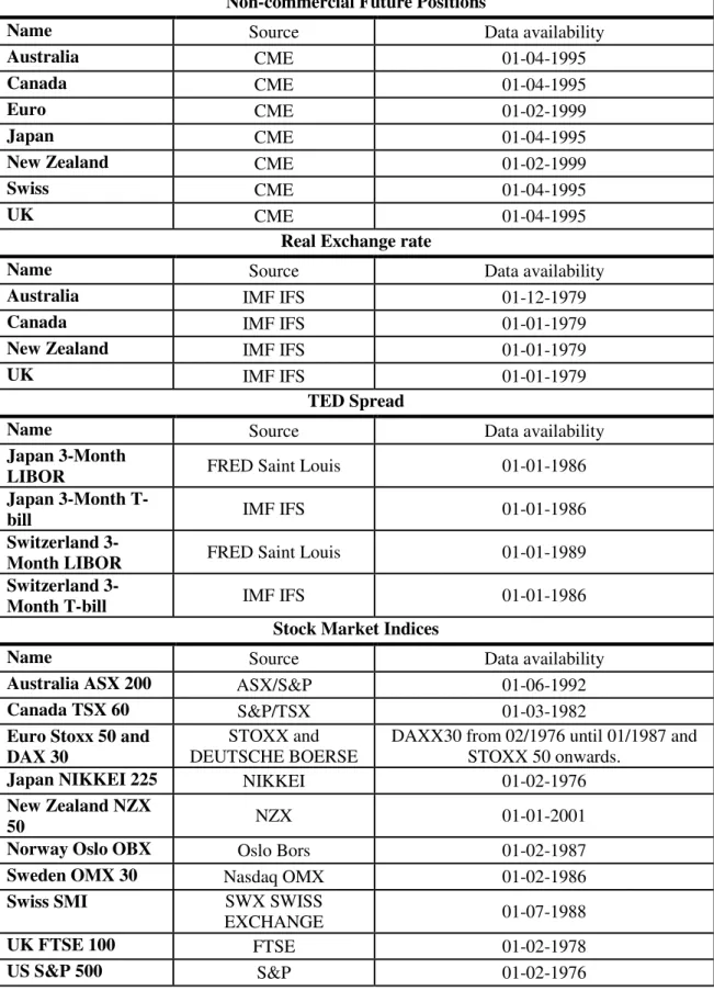
Lastly, refer to Table 1 for a description of the data used for the regime indicators’
analysis including the indicators used, the sources and dates.
V. Results of the Carry Trades
From the broad number of weighting strategies used in the carry trades it was chosen to
analyze the results of five, which are explained in section 3.2: the equally weighted
(EW), the speed weighting (SPW), the equally weighted hedged by the forward
exchange rate (EW-HF), the dollar carry trade and the rankings weighting strategy.
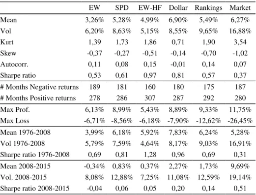
Refer to Table 2 for the observation of the correspondent results.
Firstly, it is interesting to analyze how the different strategies yield so different results
with average returns ranging from 6,90% to 3,26%, which show a similar dispersion
when accounting for the transaction costs. with a range between 5,48% to 3,19% One
can perceive that with and without transaction costs for the period under consideration
the dollar carry-trade was the strategy with the best performance in terms of average
return (6,9%) which after transaction costs decreases by 1,4%. Nevertheless,
considering the Sharpe ratio which is usually preferred due to taking into consideration
the systemic risk before transaction costs the EW-HF strategy would be preferable since
it has a Sharpe ratio of 0,97 while the dollar carry trade shows one of 0,81. When
accounting for the transaction costs the same situation persists as the former has a
18
Additionally, it is interesting also to notice that after transaction costs the dollar carry
trade does not show such a big gap in performance when related to the SPD since the
latter now has simply 0,3% lower average returns (5,17%) than the dollar carry trade
and a lower Sharpe ratio by simply 0,04 (0,60). Moreover, the rankings strategy which
presents the second highest average returns before and after transaction costs of 5,49%
and 5,33% shows at the same time the second lowest Shape ratios of 0,57 and 0,55,
respectively. The last situation is due to the high volatility of the strategy since it only
invests in a maximum of 6 currencies while from February of 1999 onwards all the
others invest in 10, the date when the Euro is first used in the strategies using forward
exchange rates.
Adding to this, it is possible to observe that all the strategies with and without
transaction costs seem to have a positive autocorrelation of one lag of 0,11 for the EW
strategy, 0,08 for the SPW, 0,15 for the EW-HF and 0,14 for the rankings’ one unless
for the dollar carry trade. The latter shows a negative but rather small autocorrelation of
-0,01 both with and without transaction costs. This may suggest that these four carry
trade strategies’ returns may be forecastable one-period-ahead which comes as utterly
important on the last section VIII when of studying the carry trade regime indicators.
Another interesting discussion is that of the portfolios’ profitability after the 2008
financial crisis and for this I calculated the returns of all the strategies for the period
after September 20087. It can be observed now that the EW portfolio is no longer
profitable even before the transaction costs with a negative average return of -0,34%.
Also when considering the EW-HF it was no longer profitable after transaction costs for
the post-crisis period with a negative average return of -0,25%. It is also interesting to
7
19
notice how does the dollar carry trade perform much better in comparison to the other
strategies as it gets an average return of 2,27% with a Sharpe ratio of 0,20 while the
rankings and SPW strategies got averages returns of 1,73% and 0,83% and Sharpe ratios
of 0,14 and 0,06, respectively, before transaction costs. In conclusion, accounting for
the transaction costs does not lead to any change on the previous pattern of te results.
Finally, when analyzing each strategy it is always interesting to compare it with the US
market excess returns. In order to do this I took the previous values from Kenneth’s
French website with monthly frequency. The statistics for the US market excess returns
are presented in Table 2 alongside the previous statistics. When considering the entire
period the market showed excess average returns of 6,27% which is higher than the
returns of all other strategies but the dollar carry trade. Alternatively, the volatility of
these returns was also almost the double of the highest volatility among strategies:
16,88% against 9,65% of the rankings portfolio. Hence, if one considers the Sharpe
ratios on the moment of taking an investment decision, the US market will rank last
with a Sharpe of 0,37. Again this situation changes after the 2008’s financial crisis since
the US average excess returns are of 9,65% and volatility is equal to 19,14% yielding a
Sharpe ratio of 0,51 which is relatively higher than the highest of the carry trade
strategies’ (0,2), the one of the dollar carry trade strategy. These results do in fact
explain the wide gap between the performance of all the carry trade strategies and the
dollar carry trade for the period after the 2008’s financial crisis since the latter has a
much stronger dependence on the dollar and, thus, it was probably this dependence
joined with the good performance of the US’ market which lead to its higher returns.
20
5.1. Evolution of the strategies over time
The high dispersion between the carry trade statistics alongside such a different
performance after the financial crisis suggests they have much different dynamics. In
order to observe this it is possible to investigate the evolution of the cumulative returns
over time assuming an investor would have 100 dollars at risk in the strategy, which is
presented in Graph 1.
The first conclusion is that in the end the dollar carry trade performed much better than
the other four strategies, which show a more similar pattern. In the beginning of the
period we observe that their evolution is pegged, however, from 1984 until mid-1993
the dollar carry trade feels an increased in value which the others did not. This is
probably explained by its high dependence on the dollar which on the other strategies
apart from the ranking’s is used just to level the investments to 0. Still, in the rankings
strategy the maximum weight it would be exposed to the dollar is equal to 50% while
for the dollar carry trade this value is 100%. Moreover, it is possible to state that the
drawdowns among strategies definitely do not follow the same patters. The dollar carry
trade strategy has much deeper drawdowns, but also one must notice that the values for
its cumulative returns are much higher. Therefore, in order to make a correct analysis it
should be pursued a relative drawdown analysis which will be taken in the chapter VII.
Additionally, while the dollar carry trade has been smoothly increased in value until
mid-2005, the other strategies have had several drawdowns without the upside trends
felt by the former, which made them less profitable.
On the other hand, the dollar carry trades felt a strong decrease in value from mid-2005
until the beginning of 2008 which was not felt by its peer strategies despite for a loss in
21
what drove returns down was the dependence on the US’s performance. Additionally,
from the SPW, EW-HF and rankings strategies it was the latter the one which suffered
the most with the 2008 financial crisis since before this event it held the highest
cumulative returns among the three and in the moment exactly after it, the previous
portfolio ranked last.
Finally, it is important to notice that in 2010 and 2012 the dollar carry trade strategy
suffered sharp drawdowns that were still not recovered by the beginning of 2015. This
result is shared by the SPW and rankings strategies due to having loss a huge share of
their cumulative returns with a drawdown in 2012. Nevertheless, the first is currently in
a downward trend while the second is on an upward one. As far as the EW and EW-HF
are concerned it seems that from a graphical analysis the EW strategy never reached
higher values than the ones of 2004 while its hedged version by 2012 had roughly
reached the pre-crisis level but due to further drawdowns it could not achieve a higher
level of cumulative returns.
In order to have a complete analysis of what lead these strategies’ returns to decrease so
sharply and to deliver a proper view on risks the strategies face, the next chapter will
comprise a brief analysis of common risk factors used in the literature to describe the
carry trade. Consecutively, in chapter VII, I develop a drawdown analysis of the five
strategies and the market’s returns.
VI. Traditional risk factors and Drawdown analysis
In this section it will be discussed whether the average returns of the carry trade
strategies previously described are explained by the exposure to the traditional risk
factors or not. In opposition to many studies in the literature here it is not intended to
22
risk factors to two: the Fama-French (1993) 3-factor model and the pure FX risk factor
as proposed by Lustig, Roussanov and Verdelhan (2011). Finally, to model this
exposition to the risk factors it was run a regression of the carry trade return for each
strategy, Zt over the source of risk, Ft, as it follows:
Zt= α + B′Ft+ εt
Furthermore, since the risk factors are explaining the returns, the α component of the
regression represents the abnormal return of the strategy, that is, the measure of the
average performance of the carry trades that cannot be explained by the unconditional
exposure to the risk factors included on the regression.
6.1. Equity Market Risk
In order to analyze if the returns from the carry trade strategies are explained by the
equity market risk it was decided to use the three Fama-French (1993) equity market
risk factors: (1) excess market return, RMRP,t, proxied by the excess return on the
market, value-weight return of all CRSP firms incorporated in the US and listed on the
NYSE, AMEX, or NASDAQ over the 1-month treasury bill rate; (2) the
Small-Minus-Big factorRSMB,t, calculated by the average return on the three small market
capitalization stock portfolios minus the average return on the three big portfolios; and
(3) the High-Minus-Low factor, RHML,t, which is developed by the average return on the
two portfolios with high book-to-market value stocks minus the average return on the
two low book-to-market value stock portfolios. Refer to Table 5.1. in order to access the
regression results.
It can be seen that as it is mostly common in the literature, the 3 Fama and French
23
strategy the t-statistic values of the factors coefficients’ range from |0,01| to |0,67| and,
thus, by not rejecting that these values are statistically different from zero it cannot be
proved that they explain the carry trade’s returns. Furthermore, the largest R2 is equal to
0, 004. Hence, the equity risk factors do not explain the carry trade returns.
6.2. Pure FX risk factors
The two pure foreign exchange market risk factors used are proposed by Lustig,
Roussanov and Verdelhan (2011) and were further used in Daniel et al. (2014) as
explanations for carry trade risk. In their study, 35 currencies are sorted in six portfolio
considering the interest rate differential and, after ranking those differentials, the
currencies were organized such that the ones with the highest rankings belong to the
same portfolio while the ones with the lowest rankings are also joined in a
correspondent portfolio. Hence, from this construction they obtained two risk factors:
(1) the average returns on all six currency portfolios, RFX−Mean,t; and the difference
between the returns of the portfolios 6 and 1, RHML−FX,t. Additionally, the authors add
that the correlation of the first principal component with FX-Mean is 0,99; while the
correlation of the second principal component with HML-FX is 0,94. Refer to Table
5.2. in order to access the regression results.
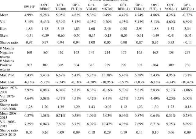
Here the results obtained from the regression are far different among strategies and,
including the transaction costs has a very weak impact in the regressions. To begin with,
for all strategies but the dollar carry trade I obtained relatively similar results to Daniel
et al. (2014) as they obtain a stronger statistical relation with the HML-FX component,
with high t-statistics.
Nevertheless, the most important result obtained from these regressions is to notice that
24
rankings both with and without transaction costs, as well as, for the SPW after
transaction costs. This suggests that the returns of these portfolios are fully driven by
the HML-FX risk factor. Yet, this result is not surprising given that the construction of
these strategies is similar to the carry trade strategy developed in Lustig, Roussanov,
and Verdelhan (2014) while the SPW, EW-HF and dollar carry trade are not. The latter
explanation is also supported in Daniel et al. (2014) while explaining the strong
explanatory power of HML-FX factor. Adding to this, the regressions delivered
relatively high R2 values ranging from 0,06 for the dollar carry trade to 0,71 for the
rankings strategy. Hence, considering everything that was mentioned it is possible to
state that strategies such as the equally-weighted and the rankings carry trade can be
fully explained by the HML-FX factor similarly to the authors results.
VII. Downside risk analysis
The carry trades are known for their high returns but also for their main drawback: the
downside risk. In fact a quick observation of the strategies’ statistics would tell us that
all have a negative skewness of -0,37; -0,27; -0,51; -0,14 and -0,70 for the EW, the
SPW, the EW-HF, the dollar carry trade and ranking strategies, respectively. The
skewness of a distribution describes the asymmetry or lack of symmetry of the returns’
distribution around the mean and, thus, it means that if negative, the carry trade returns
have a negative fat tail, that is, high drawdowns. At last, one should consider that for the
same period the market’s returns had a much more negative skewness equal to -1,02
suggesting a much higher tail risk. It is puzzling, however, how the EW-HF strategy has
a more negative skewness than its unhedged version. In order to develop a deeper study
on the downside risk three different indicators will be explored: the Sortino ratio, the
25
7.1. The Sortino ratio
One of the most popular measures of downside risk of an investment is the Sortino ratio
which follows the Sharpe ratio in that the only difference is that the former uses solely
the volatility of the negative returns, while the latter uses the volatility of the entire
sample. Hence, the larger the Sortino ratio the lower the probability of a big loss. Refer
to Table 7 in order to observe the results for this indicator for the five portfolios.
Similarly to the previous Sharpe ratio analysis we observe that the market had the
lowest value for the Sortino ratio which is explained by a higher volatility of negative
returns which accounts for a little less than the double of the carry trade strategies since
it is of 3,6% while the one of the rankings strategy is of 2,05%. In that sense, the
EW-HF strategy ranks first with a ratio equals to 4,62 while the dollar carry trade follows it
with 4,53. The strategy with the lowest value for the Sortino ratio happens to be the EW
strategy which makes now more sense than the previous analysis on the skewness,
where the latter had a better performance than its hedged version. Alternatively, the
market’s Sortino ratio is equal to 1,75 suggesting a much larger downside risk than the
one of the carry trade strategies.
Ultimately, the values for the strategies after transaction costs change in a proportional
way since the volatility of the negative returns increases or remains unchanged for all
strategies while the returns decrease in the same manner previously stated. Still, it is
relevant to note that the Sortino ratio for all the carry trade strategies after transaction
costs remained above the one of the market’s before transaction costs denoting once
again the high exposure to large drawdowns by the markets’ returns.
Nonetheless, as it was previously observed this picture changes drastically if we
26
the strategies but still kept lower than the one of the market since the latter shows a
value of 5,06% while the highest downside volatility of the carry trade strategies is
3,50%, for the SPW strategy. However, given the poor results for the average returns
the highest Sortino ratio among carry trade strategies as it would be predictable by the
higher average returns is the one of the dollar carry trade equal to 0,75 and much lower
than the one of the market: 1,92.
To conclude the Sortino analysis it is surprising that for the post-crisis period and before
transaction costs the rankings strategy has a higher ratio than the SPW strategy of 0,32
against 0,24 considering its high volatility and skew. Conversely, after accounting for
these costs the SPW strategy performs slightly better with a higher Sortino ratio of 0,19
in comparison to 0,17 of the rankings strategy.
Hence, this indicates that for the period after the 2008’s, the carry trade strategies are
exposed to a higher probability of a large loss than the US market which is not true
when considering the entire period of analysis.
7.2. Drawdowns and Pure Drawdowns
The Sortino ratio is a generally examined ratio for the comparison of the downside risk
of the strategies. Although, it does not answer some of the important questions of a
drawdown analysis such as: which strategy suffered the highest drop in value, or which
strategy took more time to recover from a severe fall? In order to answer these questions
it was decided to use two indicators used in Daniel et al. (2014), the drawdown and pure
drawdown. The drawdown is a broadly used measure defined as the decline of an
investment from its historical peak to the lowest through. This is usually measured as a
percentage between the peak and through values. It can also be measured as the number
27
drawdown is defined as a percentage loss from consecutive negative returns. Again one
can measure the number of periods of successive losses. The results for the Drawdown
analysis are presented in Table 8 and for the Pure Drawdown in Table 9. Additionally,
refer to graphs 3 and 4 for a description of the periods when these Drawdowns and Pure
Drawdowns occurred.
In the mentioned tables, the results for the biggest 10 drawdowns and 10 pure
drawdowns are shown. Once again, the market registers the highest level of downside
risk with the drawdown of strongest magnitude reaching 49% which lasted for 40
months as it started in October of 2007 and finished in January of 2011 which
representing the late global financial crisis’ losses. Also interesting is to observe that the
second biggest drawdown finished not much time before the beginning of the first since
it was equal to 47%, started in March of 2000 with the dot com bubble and only
finished in April of 2007, lasting for a much longer period of 86 months. As far as pure
drawdowns are concerned the two largest for the market were equal to 34% and 33%,
both lasting 3 months and starting in September 2009 and November 1987, respectively.
When looking at the carry trade strategies, it is interesting to notice that the largest
drawdown among carry trade strategies is not the one of the EW strategy equal to 24%
which had the lowest value for the Sortino ratio, but the rankings carry trade’s one of
36%. However, despite these two drawdowns being the strongest among the 10 biggest
for all the strategies, the longest is in fact the one of the EW strategy lasting 110
months, given that it started in December of 2005 and it did not finish by January of
2015, against 68 months of the rankings strategy which started in July of 2007 and
28
Additionally, it is surprising to note that the strongest pure drawdown of the rankings
strategy is even stronger and longer than the market’s: 39% against 34% and lasting 8
months in comparison to 3 months for the market’s strategy. Moreover considering the
loss in dollars if both strategies were started with 100 dollars, they would feel the same
loss of 249$ which is a utter negative sign for the rankings strategy given the difference
on the final cumulative returns between the strategies.
Besides, before transaction costs the strategy with the smallest drawdown with the
maximal magnitude was the EW-HF with a drawdown of 19% which lasted 46 months
and, thus, also the shortest. In second place ranks the dollar carry trade with a
drawdown of 22% lasting 59 months. Both strategies felt this drawdown also in the late
global financial crisis. As far as the second strongest drawdown is concerned the
performance remains the same suggesting that the EW-HF and the dollar carry trade
have both a better resistance to the downside risk. Furthermore, adding the transaction
costs to this picture the drawdowns are stronger and longer, however, it does not make
any of the strategies to perform better than others at the first magnitude drawdown nor
second. Finally, the EW strategy is less exposed to the downside risk than the SPW as
far as drawdowns are concerned.
When looking at the results from the pure drawdowns to the carry trade strategy it is
surprising how now the dollar carry trade performs so much better than the EW-HF
strategy since their both pure drawdown with the maximum magnitude lasts 5 months
but the one of the latter accounts only for 9% compared to 17% of the EW-HF carry
trade. In addition to this, if we consider that both strategies were initially invested 100
dollars this continued lost would amount to 119$ for the dollar carry trade pure
29
had still a higher loss given that it showed a much higher return for almost the entire
period and, thus, it would still be expected that such difference in loss would be higher.
The most unexpected part is that while this pure drawdown was felt at the same time as
the maximum drawdown for the EW-HF strategy, the same cannot be said for the dollar
carry trade once it finished in March of 2006 while the maximum drawdown was felt
during the 2008’s financial crisis. Furthermore, even the second largest pure drawdown
for the latter strategy ended in March of 1985 and the second biggest drawdown was felt
from 11/2010 and still proceeds by 01/2015 which may indicate that there is no
relationship between the pure drawdowns and the drawdowns. The same conclusions
are later found in the EW-HF strategy since the period of the second biggest drawdown
(05/1985-12/1988) does not correspond to the period of the second strongest pure
drawdown (finishing in 02/1993).
Among the other strategies, when looking at the pure drawdowns of the SPW and the
EW there are no big surprises since the SPW continues to be more exposed to this form
of downside risk with the maximum pure drawdown equal to 26% while the one of EW
is equal to 19%. What can be odder in this situation is that both last the same number of
periods: 6 months, suggesting that despite smaller in magnitude, the EW is exposed to
long periods of negative returns.
At last I explore the periods at which the biggest drawdowns and pure drawdowns
happened so to observe if it is possible to find whether there is a relationship among
these indicators or not as previously seen in the dollar carry trade and EW-HF
strategies. On the one hand, in fact for all the strategies the biggest drawdown and pure
drawdown occurred during the late financial crisis. On the other hand, the second and
30
time of the pure drawdown: the second biggest drawdown for the SPW strategy was
during 07/1985 and 03/1990 while its second strongest pure drawdown finished in
02/1993; as far as the rankings strategy is concerned the second largest drawdown was
during the same period of the SPW’s strategy while the second largest pure drawdown
was in 03/1993 as it lasted one more period than the former strategy. Yet, the third
strongest drawdown was felt at different periods among the two strategies.
In conclusion, it is possible to affirm that the carry trade strategies are exposed to strong
and long drawdowns, as well as, pure drawdowns that are still lower than the market’s
one. Furthermore, different indicators suggest different results for the strategies in that
one cannot conclude which strategy is less exposed to the downside risk by using all the
indicators at the same time. Still, the EW-HF and the dollar carry trade seem to be the
best candidates as the carry trade strategies to be less exposed to tail risk and
drawdowns. This analysis motivates the relevance of answering to the question initially
asked: how can one get the timing and, therefore, hedge from these events which
strongly drive returns down? In order to answer this question in the following chapter it
will be developed a study on the possible regime indicators capable of informing an
investor of the time a drawdown will occur.
VIII. Regime Indicators
In his book “Expected Returns: An Investor's Guide to Harvesting Market Rewards” of
2011, Antti Ilmanen describes the problem of the carry trade as being the downside risk,
which is proved by the analysis on the previous section. Furthermore, once we are
studying an arbitrage strategy these drawdowns will lead to the unwind of the carry
trade positions. As far as these unwinds have been studied, historically they are known
31
indicators useful in the prediction of next week or next month carry trade performance.
Therefore, carry trade returns are known for exhibiting short-term persistence similarly
to what was suggested by their autocorrelation and, thus, a study of the rearview mirror
indicators and stop-loss discipline is highly valuable.
In that sense, the mentioned author presents the possibility of using some variables that
allow one investor to avoid such losses which he names as regime indicators or
conditioners. The variables he presents are: overcrowded carry positions, overvalued
exchange rates from high-yield currencies, rising volatility in exchange rates, tightening
liquidity conditions especially in low-yielding “funding currency” currencies and the
changes in the stock markets’ returns for each currency. All the last indicators have also
been used in other literature either by providing a signal for the carry trade positions or
as risk factors for the carry trade returns: overcrowded carry positions and tightening
liquidity are both used in Brunnermeier et al. (2009), overvalued exchange rates from
high-yield currencies as part of the PPP condition is used in Barroso and Santa-Clara
(2013), the stock market’s returns is used in Campbell et al. (2010); and, finally, the
volatility of exchange rates is used by Bhansali (2007). Additionally, I preferred not to
use global factors also suggested by Ilmanen and used in the literature, such as the
return of the MSCI World by Bakshia and Panayotov (2013) or the US Consumption
growth by Lusting and Verdelhan (2007). The motivation for this choice is that I want
to use indicators that can be directly related with the payoffs of each currency in the
portfolio of currencies, while usually global indicators are applied when relating the risk
factor to the return of the portfolio of currencies.
Consecutively, when determining to which strategy should this study be performed it
was chosen the EW-HF strategy. This decision took into consideration four main
32
exposure on the forward exchange rate, which is important when analyzing the
relationship with the future positions’ variable; (3) by being equally-weighted, the
positions are much more flexible to change in comparison, for instance, with the dollar
carry trade which has a much higher dependence on the dollar’s performance; and (4)
despite having the strongest Sharpe ratio when considering the entire period, it presents
negative returns after the 2008’s financial crisis.
Finally, in the next part of this chapter I describe the construction of the regime
indicators and how they provide the stop-loss sign when taking the investment decision
on each currency.
8.1. The regime indicators’ variables
To begin with, when developing the signal for the speculation on overcrowded carry
positions I used the variable created by Brunnermeier et al. (2009):
Overcrowded Positiont= Fut. longTot. Fut. Positionst− Fut. shortt t
The authors use the futures position of non-commercial traders’ data from the
Commodity Futures Trading Commission (CFTC) and the intuition is that when this
value gets too high (low) it means that the carry positions are overcrowded for the
investing (borrowing) currency and, thus, the probability of a carry crash to happen
increases. The authors use the forward exchange rate positions noting that many
speculators implement the carry trade by actually borrowing and trading in the spot
currency market.
Moreover, when considering whether a currency is overvalued or not the analysis was
limited for Australia, Canada, New Zealand and UK by following Ilmanen’s advice on
33
the currencies that were the most used for investing purposes. The indicator used was
the real exchange rate and, thus, we have that if the real exchange rate is higher than 1
the currency is overvalued and, undervalued if lower.
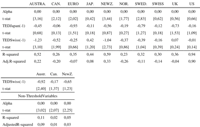
Analogously, the tightening liquidity conditions indicator should be used in
low-yielding “funding currencies” and, therefore, it was solely applied to Japan and
Switzerland since they were the most used for borrowing purposes as we can also
observe in Table 3. Here in the calculation of the liquidity conditions it was decided to
use the TED spread applied to these countries as suggested in Brunnermeier et al.
(2009), that is, the difference between the shortest term LIBOR rate available (3M) and
the risk-free rate, which is the shortest Treasury note, available for these countries. The
intuition given by the authors is that the LIBOR rate reflects uncollateralized lending in
the interbank market, which is subject to default risk, while the short term T-Bill rates
can generally be considered as risk-less since they are usually guaranteed by the
governments. Hence, when banks face liquidity problems the TED spread typically
increases, and the T-Bill yield often falls due to a flightliquidity" or flight
-to-quality".
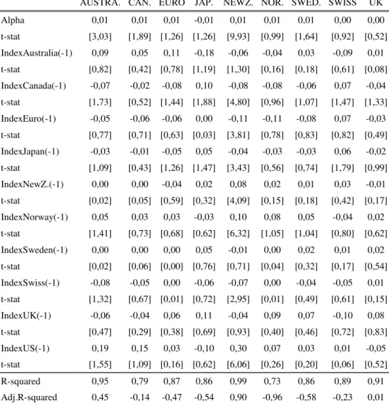
Finally, the stock market indices used were the country’s main index for a given
currency and it is available for all the currencies from a certain period described in
Table 1. Additionally, the monthly volatility of the exchange rates is also available for
all the currencies and it was calculated taking into consideration the daily values of the
exchange rates.
The next part of this chapter describes the econometric models used to find the correct
signaling provided by the regime indicators when of weighting each currency on the
34
8.2. Econometric model for the threshold signaling value
In order to use the previous indicators to provide us with the correct sign, that is, with
the prediction of a “carry crash”, what one must find is the threshold value that makes
those indicators to drive the carry trade returns down. The insight necessary for this
study is that for the different regime indicators there may be two regimes: one where the
values of these indicators have a positive relationship with the carry trade returns and
other where such relationship is negative. As an example one can consider that there is a
level for the Australian’sreal exchange rate that makes the payoffs of the Australian’s
component of the carry trade to be highly profitable; however, once passing this level,
that is, when the currency gets highly overvalued or undervalued an increase of the real
exchange rate has now a negative impact over these payoffs.
At the moment of deciding which model to use for this application, an investigation at
the literature on this topic did not show any promising result. This is due to the fact that
most of the papers on the carry trade are focused on determining the risk factors
affecting its payoffs and do not use different regimes. Nevertheless, Gubler (2014) uses
a multivariate threshold model when analyzing the carry trades based on the USD/CHF
and EUR/CHF currency pairs. However, here the author does not have a portfolio of
currencies like the one of the EW-HF strategies which requires a different analysis due
to the relationships between the currencies’ payoffs. Additionally, the author provides a
review of the most important papers using such models. Alternatively, Jordà and Taylor
(2012) use a nonlinear regime-dependent model in their approach but on the moment of
determining the threshold they do it exogenously. Finally, Clarida et al. (2009) also uses
a regime-switching model considering the exchange rate volatility as exogenous
variable. However, the latter defined these regimes in terms of the quartiles of the
35
Hence, by not having a common procedure defined among the literature a different
process was taken. This process accounts for two phases: firstly a series of VAR models
were obtained describing the relationship among each of the regime indicators and the
payoffs of every currency in the carry trade strategy under analysis; and secondly after
analyzing the results from the first phase, a threshold autoregressive model is run for the
currencies which had statistically and economically significant coefficients.
Additionally, it is important to note that due to fast market’s changes it is only
reasonable to consider values of the indicators lagged by one month. Also, from the
structural definition of the VAR model, it was necessary to include two autoregressive
components of the endogenous variables so it was decided to use the 1 and 2 months
lagged. Refer to Appendix A for a detailed description of these models.
Finally, it was decided to use the period from 03/1999-12/2003 for the regression since
it is a period when all the returns are available and which allows the thresholds to be
placed before the 2008’s financial crisis using the period when the strategies had a
regular good performance. Hence, such timespan leaves still time for using the
threshold during profitable years when making an out-of-sample analysis. In
conclusion, from this two-step approach one is able to obtain the threshold values which
give the stop-loss signal for each regime indicator for a given currency. Refer to Tables
6.1.-6.5. to observed the results of the mentioned regressions.
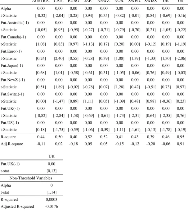
8.3. Results for the VAR and Threshold regression models
Starting this analysis with the VAR of the future positions (Table 6.1) it seems that the
only currency where the speculative positions and its carry trade returns have a
statistical significant relation is the UK with a coefficient of 0,00 and a t-stat of -2,36
36
small number of other relationships are found but these do not hold in fact any
theoretical ground given that either the statistical significance or the sign of the
coefficient do not suggest any further investigation. Therefore, it was proceeded the
Threshold regression model just for the UK’s future positions and payoffs. The results
for the previous regression indicate that there is no threshold value while having very
small and not statistically significant relation between the latter since the coefficient is
roughly equal to zero and has a t-statistic of 0,13. Hence, these regressions suggest that
there is no threshold value for the future positions on forward exchange rate that can
help one investor predicting future carry crashes in the EW-HF strategy for the period
under analysis.
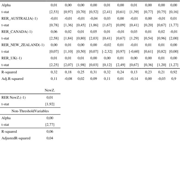
Sequentially, when studying the real exchange rate indicator, I obtain from the VAR
results (Table 6.2) that only the values for New Zealand seem to be statistically
significant with a t-statistic of -2,23 and a coefficient of -0,02, which is the expected
signal. Apart from this, the real exchange rates of Australia, Canada, New Zealand and
UK have statistically significant impact at a 95% confidence level on other currencies
but not on its own, which is not the expected result. In addition, some of these
coefficients are also positive which is not the suggested by the literature and, thus, the
threshold regression is only performed for the New Zealand dollar. Finally, when
running this regression the coefficient not only shows a positive signal (0,01) but it is
not statistically significant for a confidence level of 95%. Furthermore, no thresholds
are selected for the regression, suggesting there are no statistically significant different
regimes for this period and strategy.
When observing the results on the VAR of the TED Spread (Table 6.3) similar results
are obtained given that now, however, neither Japan nor Switzerland payoffs show a