Review
0103 - 5053 $6.00+0.00
*e-mail: [email protected]
Ultrafast Dynamics of Solvation: the Story so far
René A. Nome*
Instituto de Química, Universidade Estadual de Campinas, CP 6154, 13083-970 Campinas-SP, Brazil
A presença de moléculas de solvente na vizinhança de um soluto afeta uma variedade de processos em química e biologia, e por isso é interessante obter uma descrição física de como funciona a solvatação. Embora existam muitas ferramentas espectroscópicas estruturalmente sensíveis para a investigação do papel de moléculas de solvente em processos químicos, a medida em tempo real da dinâmica de solvatação somente tornou-se possível após o desenvolvimento de espectroscopias a laser pulsado com resolução temporal de femtossegundos. Esta revisão descreve aplicações da espectroscopia ultra-rápida ao estudo da dinâmica de solvatação. A nível de terceira ordem, discutimos a dinâmica de solvatação com técnicas ressonantes e não-ressonantes, com um foco no estudo de líquidos simples e complexos. Espectroscopias Raman de quinta ordem também são apresentadas, sendo que o enfoque dá-se no novo entendimento que estas técnicas fornecem com relação ao papel do solvente em reações químicas e à natureza anarmônica do estado líquido.
The presence of solvent molecules in the vicinity of a solute affects a variety of processes in chemistry and biology, and thus one would like to have a physical picture of how solvation works. Although there are many structurally sensitive spectroscopic tools to investigate the role of solvent molecules in chemical processes, real time measurements of the dynamics of solvation had to wait for the development of pulsed laser spectroscopies with femtosecond time-resolution. This review describes applications of ultrafast spectroscopy to the study of solvation dynamics. At third order, we review resonant and non-resonant probes of solvation dynamics, with a focus on the study of simple and complex liquids. Fifth-order Raman spectroscopies are also reviewed, focusing on the insights these techniques give into the role of the solvent in chemical reactions and the anharmonic nature of the liquid state.
Keywords: ultrafast, solvation, femtossecond, liquids
1. Introduction
Reasons for studying liquids abound. Water is essential for life and covers most of the surface of our planet. Liquids constitute a large fraction of the mass of living organisms. The volatility of most molecules is low and as a result laboratory chemical synthesis is usually performed in solutions. The rate and outcome of chemical reactions are greatly affected by the solvent.1-3 Clearly, a detailed description of the liquid state is attractive from the standpoint of intellectual ediication. Effectively, knowledge of condensed phase chemical reactions based on microscopic concepts may drive new technology in drug design and bioengineering.
Not surprisingly, liquids have been studied extensively. Some of the irst experimental studies were performed
by the biologist Robert Brown, who observed irregular motion of pollen particles loating in water.4 Since then we have discovered that liquids are wonderfully complex.5 Unlike crystals, the liquid phase is characterized by local order and long-range disorder. Its dynamic nature leads to a range of local microscopic environments. Furthermore, liquids are also dense. Therefore, approximations that are used to model gases and crystals are not easily extrapolated.
studying mechanisms of molecular dynamics. Remarkably efficient techniques for studying molecular structure are available, such as X-ray crystallography, vibrational techniques (infrared and Raman spectroscopy), and the various implementations of nuclear magnetic resonance (NMR).6-8 By the same token, the dynamics of molecular liquids have been probed by a number of spectroscopic techniques. NMR spectroscopy has been used to study rotational and translation diffusion of molecules in liquids.9 Frequency-domain approaches such as low-frequency Raman spectroscopy and dielectric relaxation spectroscopy, together with lineshape analysis in mid-infrared and Raman spectra, have also been used to study molecular dynamics in liquids.10-12
Chemical reactions occur on a variety of timescales, and accordingly many spectroscopic techniques have been developed to study these dynamical processes. At the macroscopic level, chemical reactions are described in terms of concentrations of reactant and product molecules. Each time a reactive collision occurs, the number of reactant and product molecules present in the system changes abruptly. The time intervals between successive reactive collisions can extend over a wide range of time scales - from µs (microseconds) to years - depending upon factors such as temperature, rate constant and concentration of chemical species involved in a given reaction.
At the molecular level, reactive encounters lead to the formation of an “activated complex” or “transition-sate”, which then dissociates into product molecules. For example, charge transfer reactions are a special class of chemical reactions in which the transition occurs only in a nuclear coniguration where the electronic energies of the reactant and product states are degenerate. This follows from the requirement that (i) the reaction conserves energy and (ii) that a separation of time-scales for electronic and nuclear motion exists (i.e., Born-Oppenheimer approximation).13 On the other hand, many reactive events can be described by nuclear motion on the potential energy surface of a single electronic state.14 The same potential energy surface also governs harmonic motions (normal modes) commonly measured by infrared and Raman spectroscopies. Given the weights of atoms and common bond energies, these vibrational motions occur on the time scale of femtoseconds (fs) to picoseconds (ps). Therefore, the experimental challenge of designing a spectroscopic tool that probes dynamical molecular information in real time requires the access to femtosecond time scales.
Several advances in laser technology over the last few decades have made the generation of stable femtosecond pulses across the visible and infrared spectral regions a routine effort.15 Femtosecond or ultrafast spectroscopy
allows induced molecular motions to be observed directly,16 thus providing insightful information which adds to the large body of knowledge of reaction mechanisms obtained by conventional chemical kinetics techniques. Incidentally, the connection between femtosecond spectroscopy and chemical kinetics is clear: ultrafast spectroscopy experiments that probe the time-evolution of diagonal elements of the system Hamiltonian measure kinetics in much the same way as conventional chemical kinetics experiments. Therefore, the chemistry principles that we learn are transferable, and we can use knowledge gained from one approach to understand the other. The techniques used in each case are nonetheless different: whereas a laser pulse triggers synchronization of the system that ultimately allows the realization of an ultrafast time-resolved detection, chemical kinetics experiments do not require synchronization, and the dynamics are correspondingly much slower.
This brief review chronicles the remarkable technical and conceptual developments in femtosecond time-resolved spectroscopy that are providing insights into the basic molecular motions that characterize the liquid state. Solvent and solvation dynamics of small polar molecules, as measured by third-order resonant and non-resonant spectroscopies, are reviewed in sections 2 and 3, respectively. Applications to more complex solvents are reviewed in section 4. Fifth-order spectroscopies are then discussed together with their application to the study of pure liquids and the role of the solvent during chemical reactions in solution. In order to introduce the reader to the subject, the supplementary information briely reviews concepts and methods in time-resolved nonlinear spectroscopy. The structure of the review is idiosyncratic to the author yet many recent achievements are also discussed. Hopefully, this format will help those who want to be introduced to the ield while providing up-to-date information.
2. Polar Solvation Dynamics from the Solute
Perspective
scales are extremely useful in practice, and solvent polarity tables are commonly used as a reference when a chemist chooses a solvent, for instance, for chemical reactions or chromatographic separations.
2.1. TRFS
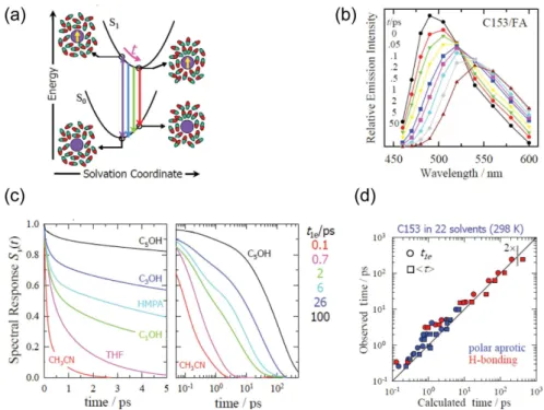
More recently, solute-solvent interactions have been studied with high time resolution, particularly after the development of mode-locked femtosecond lasers. For example, time-resolved luorescence spectroscopy (TRFS) has provided insights on solvation dynamics as well as solvent polarity scales.18 Figures 1a and 1b illustrate the basic idea and raw data behind TRFS studies of solvation dynamics. Upon absorption of a photon, electronic excitation of a suitable dipolar solvation probe leads to a nearly instantaneous change in both magnitude and direction of the probe’s dipole moment. For example, in the case of coumarin dye C153, which is a commonly used solvation dynamics probe, both magnitude and direction of its dipole moment change upon electronic excitation (8 D calculated, ca. 7 D observed).19 By contrast, the solvent molecules in the vicinity of the solute remain ‘frozen’ in their initial conigurations immediately after this signiicant charge redistribution in the excited state (Born-Oppenheimer approximation), thereby leading to an increase in the solvation energy of the probe (Figure 1a).
In the TRFS technique one probes the emission spectrum shortly after electronic excitation by a “pump” pulse. Typically, emission is probed at various wavelengths across the luorescence spectrum;20 alternatively, the entire emission spectrum has been collected in a single shot by broadband up-conversion methods.21-23 Figure 1b shows a solvation dynamics experimental result, in which the time-resolved emission spectra of C153 in formamide shift to longer wavelengths as a function of time after chromophore photo-excitation. Therefore, TRFS measures the time-evolution of spectral shifts that occur as the solute relaxes on the excited state potential energy surface. A quantitative analysis of time-dependent spectral shifts yields the solvation dynamics function, which informs us on how the solvent responds to changes in the solute’s electronic structure.24
The large body of ultrafast TRFS work performed with a variety of solvents shed light on the fundamental timescales of solvation dynamics.18 A qualitative inspection of this rich data set already indicates that polar solvation dynamics is essentially biphasic in nature (Figure 1c). Typically, the early time response decays within a few hundred femtoseconds, whereas the slow component decays on a picosecond-nanosecond time scale. The fast component is pronounced in many solvents, and as a result, solvation is essentially complete a few picoseconds after electronic excitation of the dye used as a solvation dynamics probe. The second
component, on the other hand, is solvent dependent: the characteristic timescale for this component is on the order of 1-10 ps for aprotic solvents, although it reaches much longer values as the solvent viscosity increases.
Our knowledge of solvation dynamics has been signiicantly augmented by theoretical and computational work. Interestingly, the essential features of the experimental data described in the previous paragraph are captured by dielectric models (Figure 1d).13,17,18 In such models, the solute is described by a point-dipole, whereas the solvent is described by a frequency-dependent dielectric constant ε(ω) (or, more generally, ε(r, ω)),25 where the solvent response is parameterized with dielectric relaxation experimental data26 that now extends into the terahertz (THz) range.27,28 These models it experimental solvation dynamics data surprisingly well, thus highlighting the intrinsically dipolar nature of solute-solvent interactions.
In addition to phenomenological models and microscopic theories, molecular dynamics simulations have been very useful in providing a “solvation mechanism”, that is, a microscopic picture of the fundamental molecular motions that lead to the measured response times.29 As in the experiments, the calculated solvent relaxation also shows a biphasic character, with a fast and prominent decay followed by slower relaxation. The fast, so-called “inertial”, component is associated with the frictionless librational motion of solvent molecules. This collective motion was found to be faster in acetonitrile than in methanol and butanol due to hydrogen bonding in the alcohols, although the solvent-dependence is weak and the decay occurs within a picosecond. By contrast, in water the inertial is dynamics much faster than in aprotic solvents. This is expected since any inertial libration of a hydroxyl (OH) group ought to be faster than any inertial motion of an aprotic group due to the small mass of hydrogen (H). Moreover, given the short time associated with the fast component, the amplitudes of solvent rotations are correspondingly small. On the other hand, the slowest component, often referred to as “the second phase of solvation”, is associated with diffusive molecular motion and is thus solvent-dependent.
2.2. PE spectroscopies
In parallel with the TRFS studies described above, solvation dynamics also began to be studied with a general class of coherence spectroscopy techniques, most notably with photon-echo (PE) spectroscopy. Some of the contributions of PE spectroscopy to solvation dynamics include:30,31 (i) insights into the relationship between optical dynamics and solvation, (ii) the experimental determination of solute-solvent interactions (spectral
density), (iii) fundamental solvation timescales, and (iv) the connection between various spectroscopic probes of solvation dynamics.
In analogy with work performed in the radio frequency range,32 PE spectroscopy33 was originally developed to distinguish homogeneous and inhomogeneous broadening mechanisms (fast and slow processes, respectively) that underlie the absorption linewidth. Photon-echo spectroscopy can be thought of as a “pump and probe” experiment in which the pump pulses modulate the absorption spectrum of the chromophore, and a constructive interference induced by the probe pulse is then measured to give the echo signal.34 The amplitude and contrast of the fringe pattern created by the pump pulses diminish with time due to solute-solvent interactions thus leading to a decrease in the amplitude of the emitted echo signal.
Experimentally, the spectral-interferometry PE design uses the “pump and probe” coniguration described above, with a detection scheme that measures the frequency domain interference between probe and echo signals.35 Other commonly used implementations employ a noncollinear geometry for all three pulses in order to enhance the echo signal-to-noise ratio by reducing background signals, utilizing different detection schemes: time-integrated,36 time-gated,37,38 and heterodyne-detected PE.39,40 More recently, ield-resolved PE measurements allowed a full analysis of the optical dynamics analogous to 2D NMR techniques.41 Diffractive-optic elements were particularly helpful in the design of phase-stable, two-dimensional PE interferometers.42-46
model is used to analyze experimental solvation correlation functions by representing intramolecular vibrations and solvent motions in terms of under- and overdamped Brownian oscillators, respectively.42 This model has been applied to a number of systems, capturing essential features of solvation dynamics of liquids that can be represented as harmonic baths.50 Despite its success, variants of the formalism that consider anharmonicity of the liquid state potential51-53 and additional electronic resonances in-/outside the laser bandwidth have been discussed.54,55
Figure 2 shows 3-pulse PE peak shift (3 PEPS) vs. population time T data from IR144 for several different polar solvents: methanol, ethanol, butanol, and ethylene glycol. The 3PEPS data from IR144 in different solvents have common features. First, the 3PEPS decays with several well-separated time scales. Second, the 3 PE peak shifts for different solvents are almost identical, and thus solvent-independent, for T up to ca. 500 fs (Figure 2, bottom) although the amplitudes of this ultrafast component are solvent-dependent. Third, the oscillatory component at short times (Figure 2, bottom) is solvent-independent and attributed to intramolecular vibrations in IR144. Fourth, the 3PE peak shifts for different solvents are clearly different at longer population times (Figure 2, top). The picosecond processes are in the slow modulation limit and constitute Gaussian inhomogeneous broadening in the absorption spectrum.
More generally, solvation dynamics studies with PE spectroscopy have been performed with a variety of small polar solvents.30,31,56 The broad picture revealed by this class of measurements is that, for small polar liquids, solvation dynamics occurs in a bimodal fashion with two characteristic time scales. The ultrafast component decays on a ca. 100 fs time scale; interestingly, this early-time response was observed in a variety of solvents. The ultrafast response is followed by a slower component decaying on a picosecond-nanosecond time scale. Therefore, the PE results are consistent with the time-resolved luorescence observations, thus indicating that PE spectroscopy was useful in providing an independent measure of the fundamental timescales associated with the bimodal solvation model described in the previous section. In fact, a formal connection was established between TRFS and PE observables (solvation function and solvent equilibrium correlation function, respectively).30,31 Taken together, the experimental and theoretical work enabled lexibility in the design of solvation dynamics experiments. For example, TRFS can be studied with commercially available instruments, and is generally considered to be simpler to implement. On the other hand, the early-time solvation response, studies of equilibrium solvent luctuations, and systems displaying small Stokes shifts are best studied with PE spectroscopy.
Another attractive feature of PE spectroscopic studies of solvation dynamics is that a Fourier transformation of the measured solvent luctuation correlation function directly yields the spectral density. The spectral density describes the spectrum of solvent motions coupled to the perturbed solute, and therefore provides insights on the nature of solute-solvent interactions in solvation (see below). PE spectroscopy thus provides a direct experimental test bed for microscopic mechanisms of solvation inferred from molecular dynamics simulations.
3. The Solvent’s Perspective
Fluorescence and PE spectroscopies, together with theory and molecular dynamics simulations, have provided a fairly comprehensive description of the “mechanism” of polar solvation dynamics. Nonetheless, these experimental approaches provide an indirect view of fundamental molecular motions of the solvent. That is, in both experimental techniques, a “reporter” solute is used to extract the response of the solvent to a perturbation in the solute’s electronic structure. Linear response theory is then used to infer the fundamental motions and luctuations of liquids in the absence of the solute, which is regarded as a small perturbation to the solvent structure.
Two other commonly used tools to study dynamics of the liquid state have provided complementary perspectives on solvation dynamics: ultrafast terahertz and vibrational spectrocopies. These two approaches probe the ca. 0-500 cm-1 spectral window, which is also accessible by fluorescence and echo spectroscopies upon Fourier transformation of the time-domain data. The importance of this spectral region for solvation dynamics is that continuous changes in local density at room temperature are associated with excitation of low-frequency intermolecular motions of liquids. Therefore, terahertz and vibrational spectroscopies provide a direct view of solvent and solvation dynamics from the perspective of the solvent, thus complementing the insights based on luorescence and echo techniques. In order to study directly the vibrational motions of the solvent, long wavelength sources are required. Nonlinear mid-infrared spectroscopy is an ideal technique for studying intramolecular motion of aqueous solvation shells.57,58 On the other hand, low-frequency nuclear motion of liquids and solutions has been interrogated directly with THz59-61and Raman probes.62-64
3.1. OKE spectroscopy
In parallel with work on resonant probes of solvent dynamics (TRFS and PE), non-resonant probes were developed to give information about solvent dynamics from the solvent’s perspective. Time-resolved optical Kerr effect spectroscopy (OKE) has been particularly successful for the interrogation of ultrafast molecular dynamics of liquids.65-67 The main contributions of OKE spectroscopy to solvation dynamics can be summarized as follows: (i) experimental determination of the solvent spectral density, the spectrum of solvent motions in pure solvents and solutions, (ii) fundamental timescales of solvent dynamics from the perspective of the solvent, (iii) role of polarizability in solvation, (iv) the connection between various probes of solvent dynamics.
The technical implementation of OKE spectroscopy is continually evolving68,69 but the basic design can also be described as a pump and probe measurement whereby linearly polarized pump pulses induce a transient change in the solvent’s refractive index (birefringence), while the probe pulse monitors the decay of the real part of material’s polarization response.70-74 OKE spectroscopy is thus essentially a time-domain Raman experiment probing the anisotropic component of the polarizability time correlation function. Upon Fourier transformation, the OKE response gives the spectral density of the liquid in the 0-500 cm-1 window, which contains information
about solvent molecular motions that can be excited at room temperature. In that sense, solvent dynamics probed by OKE provides complementary insights into solvation dynamics probed by other techniques. Low-frequency solvent motions couple to the solute molecules that are probed by luorescent and echo spectroscopies, which thus infer solvent dynamics from the perspective of the solute. On the other hand, the spectrum of intermolecular motions of the solvent can be probed directly with non-resonant techniques such as OKE. A formal connection between these various third-order nonlinear probes of ultrafast solvation dynamics has been forged.75,76
Figure 3 shows time-resolved OKE spectroscopy results for sulfur dioxide and chloroform.65 The experimental results shown in Figure 3 have three characteristic features: (i) an electronic response associated with the instantaneous nonlinearity of the liquid, (ii) a prominent sub-picosecond component, and (iii) a slower component that decays on the picosecond timescale. Since most solvation dynamics studies focus on molecular (rather than electronic) motions of the liquid, contributions (ii) and (iii) are typically deconvoluted from (i) and subject to further data analysis. MD calculations show that the fast component is associated with single-molecule (e.g., rotational) relaxation together with collective (translational or rotational) molecular motion, which is commonly referred to as ‘interaction-induced’ solvent motion. The slow component of the OKE response, in turn, corresponds to the diffusive molecular reorientation of the solvent, as evidenced from its viscosity dependence. Therefore, as in solvation dynamics studies probed by luorescence and echo spectroscopies, the solvent response probed by OKE is largely biphasic, with a prominent fast contribution and a slower diffusive component. Moreover, the polarizability response of the solvent probed by OKE spectroscopy, in conjunction with MD simulations and data analysis, reveals that many solvent motions contribute to the early-time response.
4. Applications of Ultrafast Spectroscopy to
Solvation Dynamics in other Systems
In addition to studies on polar solvation dynamics, there is an ample variety of systems, ranging from the simple to the complex, that have been the focus of solvation dynamics investigations using TRFS, PE and OKE spectroscopies, among others. In a sense, these studies indicate our interest in, and importance of, the dynamics of solvation. The subject of ultrafast solvation dynamics in solvents other than small polar molecules is very extensive and cannot be covered adequately in a single review. Therefore, we will use our knowledge gained from work on polar solvation dynamics as a starting point to try to rationalize results obtained for other classes of solvents. The focus will be on assessing whether the lessons learned from studies with polar solvents are transferable to other systems, and how much so.
4.1. Nonpolar solvents
Studies of nonpolar solvation dynamics have been performed for several aromatic and aliphatic hydrocarbon solvents, and with several ultrafast techniques such as transient hole-burning,77 fluorescence,78,79 THz,80 and PE.81,82 This body of work showed that solvation dynamics
is non-exponential in nonpolar solvents. The time-domain data is typically described by a model with two predominant timescales, with the fast and slow components describing inertial and diffusive dynamics, respectively. In that sense, experimental work on ultrafast nonpolar and polar solvation dynamics share many similarities.
On the other hand, continuum83 and microscopic84 models as well as simulations85,86 indicate that very different mechanisms underlie the similar-looking temporal proiles of polar and non-polar solvation dynamics. For example, dielectric continuum models used to successfully describe polar solvation dynamics are based on dipole-dipole interactions between solvent molecules. Therefore, such models cannot describe nonpolar/nondipolar interactions and dynamics adequately. A hydrodynamic model based on mechanical, rather than dielectric, relaxation formed the basis for a viscoelastic theory of nonpolar solvation.87 The microscopic picture of this model describes the early-time dynamics by a change in the solvent cavity, and the slower component is described in terms of diffusion. The model has successfully described experimental results at high viscosities but not at low viscosities. On the experimental side, novel ifth-order spectroscopic techniques have been proposed to test the hypothesis that the inertial phase of solvation in nonpolar solvents is associated with changes in solvent cavity/size (see below).
4.2. Mixtures of simple liquids
Solvation dynamics in binary mixtures of small solvent molecules has been studied by a number of groups. The studies reported so far span polar-polar88-90 polar-nonpolar91-94 and nonpolar-nonpolar95 binary mixtures. The experimental results for solvation dynamics in binary mixtures are similar to those obtained for the pure liquids separately. That is, the solvation response is non-exponential, with basic features of the data being described by a prominent sub-picosecond fast component followed by a small amplitude, slower (several picoseconds) component. A mechanistic description of these processes, based largely on molecular dynamics simulations, identiies the fast component as reorientation of solvent molecules in the vicinity of the solute, whereas diffusive motion across the solvation shell takes place at longer times. When two solvents of very different polarities are used, the phenomenon of preferential solvation is useful for understanding more mechanistic details. For example, solvation dynamics of C153 in acetonitrile:benzene mixtures involves inertial reorientation of acetonitrile (MeCN) molecules in the solvation shell, whereas the slower component is associated with diffusion of the more polar acetonitrile into the solvation shell.96
4.3. Ionic liquids
Ionic liquids have received much attention from the scientiic community in the past few decades.97-99 Ionic liquids are highly polar and highly polarizable as well, thus being uniquely suited to dissolve a variety of chemicals having different stereo-electronic properties. These types of liquids have been regarded as “green” solvents since they are enabling synthetic chemistry without the need for organic solvents that contaminate the environment.100 Clearly, the key physico-chemical property of ionic liquids is their solvation free-energy, and thus solvation dynamics studies have increased tremendously in the past few years.101
Utilizing OKE and TRFS ultrafast spectroscopy techniques, the fundamental solvation timescales have been characterized for many ionic liquids (e.g., imidazolium- and phosphonium- based ionic liquids), and a few trends are beginning to be observed.102-109 First, solvation dynamics in room-temperature ionic liquids are much slower than observed for conventional liquids due to the high viscosity of ionic liquids (Figure 4). Second, temporal proiles are highly non-exponential. Interestingly, the discussion on the number of components underlying solvation dynamics in ionic liquids is ongoing. Nonetheless, the biphasic character of solvation dynamics in simple liquids forms the basis of
mechanisms proposed for solvation in ionic liquids. That is, a fast component associated with free motion of solvent molecules in the vicinity of the solute, and slow motion due to diffusive transport. Data itting including three or more parameters point to a more complex mechanism whereby coupled inertial-diffusive motions may also contribute to the observed dynamics. The fastest component occurs on a sub-picosecond timescale, as observed in solvation dynamics studies of simple liquids, whereas the slow component is much slower than that observed in conventional solvents. The second phase of solvation commonly observed in small polar solvents is diffusive in nature and thus depends on the solvent viscosity. Ionic liquids are much more viscous than conventional solvents, thus suggesting that diffusion may be relevant at long times during solvation dynamics in ionic liquids. On the other hand, it is somewhat surprising to see that ionic liquids have an ultrafast, sub-picosecond component, which is commonly seen in conventional liquids. A detailed mechanistic understanding of this contribution to solvation dynamics will likely be pursued in the near future. Based on previous ultrafast spectroscopic studies of solvation in polar and non-polar liquids, it has been suggested that the ultrafast component is associated with inertial motion of solvent molecules in the vicinity of the solute. Given the ionic nature of these ubiquitous liquids, translational inertial motion may play a major role, although a more accurate picture including the non-spherical shape of ionic liquid constituents may reveal that a coupled translation-rotation inertial motion is effected at the shortest solvation timescales.
two liquids are compared, presumably due to differences in intermolecular interactions for the ionic liquid relative to the homologous neutral binary solution.
On the theoretical/computational front, there have already been a number of simulation studies that have sought to interpret the solvation dynamics observed in ionic liquids.110,111 Shim et al.,110 have performed molecular dynamics simulations of 1-ethyl-3-methylimidazolium chloride (EMI+Cl–) and 1-ethyl-methylimidazolium hexafluorophosphate (EMI+ PF
6
–) using probe solute
molecules. The authors have found that solvation dynamics in EMI+Cl– and EMI+PF
6
– is biphasic, with
a sub-picosecond inertial regime followed by a slow diffusive regime. The speciic location of ions involved in subpicosecond solvation dynamics were found to be dependent on the solvent density. Ions in the vicinity of the solute governed solvent dynamics especially at higher densities, whereas at low densities ions farther away from the solute also participated in the solvation process. Kobrak has characterized the solvation dynamics of 1-butyl-3-methylimidazolium hexafluorophosphate (BMIM PF6) in response to photoexcitation of C153 via molecular dynamics simulations.111 This study has shown that the short-time solvation dynamics of BMIM PF6 is largely collective on all time scales, in contrast with solvation dynamics in small polar solvents where independent motions of solvent molecules also contribute to solvent dynamics. Moreover, the fastest solvent response
is characterized by rovibrational motion followed by ionic translation which is the dominant signal contribution at short times. Again, a contrast is observed when solvation dynamics of ionic liquids and polar liquids are compared, as the dynamics of polar solvent molecules are largely characterized by rotational motion.
4.4. Surfactant assemblies
Solvation dynamics in surfactant assemblies have proven to be particularly challenging to rationalize on the ultrafast time-scale.112,113 The systems (micelles, reverse micelles, vesicles) studied so far with ultrafast spectroscopy share at least three features: these are large, charged and lexible systems. Since these properties are in contrast with those of commonly used solvents, new solute/solvent effects are seen: (i) some of the solvent degrees of freedom are frozen at the solute/solvent interface, (ii) counter-ions may be present near the interface, and (iii) the lexibility of the solvent molecules leads to an ill-deined, “dynamic” interface. Interestingly, a connection between solvation dynamics and these new effects has proven dificult to forge, despite the enormous amount of work in this area in the past decade.
Most of the work on ultrafast dynamics of surfactant assemblies has been carried out in aqueous solutions. Although it is dificult to disentangle the role of these “novel” effects described in the previous paragraph, much
progress has been made. Several studies have revealed the role of effect (i) above on solvation dynamics. Using 3PEPS as a tool to probe solvation dynamics near lecithin vesicles, Vohringer and co-workers114 have reported a two-time scale decay (prominent and fast inertial component followed by a slow diffusive component), which was attributed to perturbed water structure with reduced hydrogen bonding between water molecules.
The body of work in this area, taken collectively, indicates that effects (ii) and (iii) give rise to complicated dynamics, possibly due to heterogeneity in water structure near the charged, lexible interfaces. The dynamic nature of the intermolecular interactions in reverse micelle implies, for instance, that the Stern layer containing surfactant head groups, counter-ions, and water will have properties intermediate between those of water and hydrocarbon.115 Moreover, the diffuse electrical double-layer that is formed extends into the aqueous phase, leading to spatial heterogeneity. Thus, the major problem in understanding solvation dynamics in reverse micelles is properly describing interfacial concentrations and distributions. Recent MD simulations and ultrafast infrared spectroscopy measurements have indeed shown position-dependent water dynamics as water molecules were distributed in different parts of reverse micelles.116-118
5. Fifth-Order Spectroscopies: Why and How
In spite of the enormous success in tackling long-standing challenges to our underlong-standing of liquid-state dynamics, third-order ultrafast time-resolved spectroscopies suffered from a dificulty which is also faced by frequency-domain approaches designed to study dynamical aspects of the liquid state: these measurements involve a single variable - time or frequency - and thus are incapable of uniquely identifying line broadening mechanisms (see below).
It is possible to gather information about rapid motion and dynamics by working in the frequency domain. The low-frequency motions of liquids are excited at room temperature thereby leading to continuous changes in local density. Even before the discovery of the laser, optical techniques such as dynamic light scattering (DLS) were developed to measure these luctuations of liquid density.119 The depolarized DLS technique accesses the same dynamics as OKE spectroscopy. Thus, in principle, the information content of OKE and dynamic light scattering measurements is the same and connected by a Fourier transformation.120,121
In practice, however, time- and frequency-domain spectroscopies contain complementary information, and
each technique has advantages and disadvantages. For example, Kinoshita et al.,122 have performed systematic comparisons of OKE and DLS measurements for supercooled liquids. More recently, Brodin and Rössler have also directly compared OKE, DLS and dielectric spectroscopy data for glass-forming and liquid-crystal-forming systems. Good agreement was found in the mesoscopic dynamic range (ca. > 100 ps),123 in which an intermediate power law of the OKE response functions was shown to be equivalent to excess wings in the frequency-domain measurements, with subtle differences observed at frequencies > 10 GHz.124 This body of work showed that femtosecond time-resolved spectroscopy is suited to study the earliest events in solvent and solvation dynamics, whereas frequency-domain approaches were most useful at higher frequencies. As shown above, essentially the same conclusion was arrived at when comparing time-resolved luorescence spectroscopy and dielectric spectroscopy. Though the information content of these time- and frequency-domain spectroscopies is the same, systematic comparisons lead to a richer data set for understanding liquid state dynamics than any technique could provide alone.
As mentioned previously, the relationship between these time- and frequency-measurements is given by a Fourier transform. More generally, Loring and Mukamel have shown that techniques involving only a single time or frequency variable give insights into the total response due to all broadening mechanisms.120 Alas, experimentally measured responses may be caused by different physical phenomena, such as lifetime broadening, dephasing, and inhomogeneous broadening.120 The determination of line broadening mechanisms in optical spectroscopy was accomplished by the development of resonant two-dimensional ultrafast spectroscopies, such as three-pulse PE measurements, analogous to multi-dimensional approaches in NMR (section 2.2). Thus, two-dimensional ultrafast spectroscopies intrinsically possess more information than their one-dimensional counterparts. Recent linear pulse propagation measurements were also best understood in a joint time-frequency representation.125 Ultrafast 2D visible and infrared spectroscopies are third-order techniques that allow the direct measurement of electronic and vibrational couplings in small molecules and complex systems.
5.1. 2D Raman spectroscopy
motions and intermolecular couplings in the liquid state.126 In that sense, the proposed experiment was similar to resonant third-order 2D IR and PE spectroscopies, the important difference being that 2D Raman is an off-resonant, ifth-order measurement. An oversimpliied but perhaps useful description of the 2D Raman experiment can be obtained by regarding it as a “pump-pump-probe” measurement. In this picture, the irst two Raman “pump” pulses generate a vibrational coherence between ground and excited states, the second pair of Raman “pump” pulses generate a coherence between ground and Raman overtone states, and inally the “probe” pulse induces the signal arising from the nested ifth-order material response. By designing a pulse sequence that enables population of Raman overtone frequencies, one can in principle probe anharmonic motions relevant to liquid state dynamics. This description hopefully serves to illustrate the connection between utrafast 2D Raman signals, anharmonicity of the liquid state potential, and the ifth-order nonlinear polarizability.
So far, three liquids have been studied with ifth-order 2D Raman spectroscopy, namely, carbon disulide,127-129 benzene,130 and formamide.131 The homodyne-detected ifth-order Raman signal of formamide for the R(5)
zzzz tensor element is shown in Figure 5.131 The experimental results shown in Figure 5 have three distinctive features: (i) an absence of signal along τ2, the time delay between the two “pump” pulses (four Raman pulses). Previously, it had been shown that four-wave mixing signals along τ2 may dominate the overall response of the 2D Raman experiment on carbon disulide thereby masking the information content of the ifth-order data.132 In contrast, the results shown in Figure 5 provide clear signatures of the Raman echo. (ii) A dominant signal parallel to the time delay axis between the second set of Raman “pump” pulses and the “probe” pulse. (iii) A smaller, short-lived signal along the diagonal. By comparing the results with previous work and molecular dynamics calculations, these observables have been interpreted respectively as (i) absence of lower-order cascade signal contributions, (ii) vibrational anharmonicity, and (iii) nuclear rephasing ability of the solvent indicating the separation of homogeneous and inhomogeneous contributions to the signal. Interestingly, the overall ifth-order response is qualitatively similar in the three solvents studied thus far (carbon disulide, benzene, and formamide). A more quantitative comparison of the 2D Raman data from different solvents indicates that stronger intermolecular interactions, and hence more structured liquids, lead to longer-lived Raman echoes as well as larger ifth-order signals.
5.2. PORS and RAPTORS
In addition to the characterization of fundamental anharmonic motions of the liquid state by ifth-order 2D Raman spectroscopy, ifth-order probes of solvent dynamics in solvation and chemical reactions have been recently developed, such as polarizability response spectroscopy (PORS),133 and resonant-pump third-order Raman probe spectroscopy (RAPTORS).64 While the large body of work on time-resolved luorescence and PE spectroscopy has provided insights into solvation dynamics from the perspective of the solute, OKE spectroscopy gave much insight on the spectral density of pure liquids. PORS and RAPTORS, in turn, measure spectral densities of liquids during solvation/reaction by selectively measuring the solvent response in the vicinity of the solute/reactant. Therefore, PORS and RAPTORS provide a direct view of the intermolecular spectrum of solvent modes that couple to solvation and chemical reaction dynamics. Also, femtosecond stimulated Raman spectroscopy (FSRS)134 is a recently developed technique that has been applied to the study of high frequency (> 200 cm-1) vibrational resonances.135 In principle, FSRS can also measure the same polarization response as in PORS and RAPTORS; in practice, FSRS signals have been recently interpreted as arising from four-wave mixing processes.136,137 We also note another recently developed ifth-order spectroscopy MUPPETS (Multiple Population-Period Transient Spectroscopy) which allows quantitative analysis of heterogeneous and homogeneous dynamics characterized by nonexponential relaxations.138
Both PORS and RAPTORS can be thought of as “pump and probe” experiments in which electronically resonant pump pulses induce charge redistribution in the excited state of a given solute/reactant, while “probe” pulses measure the coherent Raman response of low-frequency solvent motions perturbed by the pump-induced charge
Figure 5. Homodyne-detected ifth-order Raman signal of formamide for the R(5)
zzzzz tensor element.131 Reprinted with permission from Li, Y.
redistribution. Although the experimental implementation of PORS and RAPTORS differ, a formal connection between the two techniques has been described recently.139 Within the “pump and probe” picture described above, the pump pulses induce electronic excitation of the solute/reactant. Therefore, ground- and excited-state polarizations are 180o out-of-phase with respect to each other; these phase changes of π in the electric ield, in turn, cause the polarization envelopes to change sign. As a result, after a time delay T the “probe” pulses measure the difference in Raman spectra of the solvent in the vicinity of reactive and unreactive solute molecules. Therefore, PORS/RAPTORS are only sensitive to solvent motions occurring in the vicinity of the solute/reactant.
Recently, Blank and co-workers63 have studied excited state hydrogen bond dynamics of Coumarin 102 (C102) laser dye in pure acetonitrile as well as acetonitrile:water binary mixtures from the perspective of the solvent, using RAPTORS.63 The measurements of C102 in acetonitrile:water mixtures performed at a range of concentrations (xMeCN = 0, 0.25, 0.5, 0.75, 1) revealed an initial fast rise of the signal followed by an exponential decay.140 The initial negative change seen at all molar fractions studied relects the dipolar solvation component of the solvent response. The increase in C102’s dipole moment upon photoexcitation increases the intermolecular solute-solvent interactions, thereby tightening the local solvent structure in the vicinity of the solute and thus decreasing the Raman response of the solvent. Moreover, additional dynamics is seen in solutions with higher water content (xMeCN = 0.50 and 25). The increase in the intermolecular solvent response seen for these two solutions was associated with a loosening of the solvent environment,141 which in turns relects excited-state hydrogen bond breaking dynamics. Monte Carlo simulations of the C102:binary mixture indicated that the carbonyl site of C102 likely participates as a donor in two hydrogen bonding interactions with water.
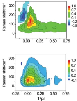
Scherer and co-workers142 have recently applied ield-resolved PORS to the study of solvent dynamics coupled to a photo-induced electron transfer reaction in two solvents: acetonitrile and methanol (MeOH) (Figure 6). This work followed a previous PORS study of solvation dynamics in C153,132 with a new design based on previous work on electric-ield resolved transient gradient spectroscopy and coherent Raman Stokes spectroscopies.143,144 The solute, 1-ethyl-4-(carbomethoxy)pyridinium iodide (ECMPI), was chosen because the electron-transfer reaction can be photo-induced in this system. Solute dynamics of ECMPI in methanol and acetonitrile have been previously characterized, where the electron-transfer rates were found to correlate with the acceptor-donor distance, and the charge
transfer reaction was found to be nearly a factor of ten times faster in acetonitrile than in methanol.55
Interestingly, PORS spectra for ECMPI in acetonitrile and methanol revealed that the polarizability spectral density was time-dependent (Figure 6). The general trend observed in both solvents was that of an initial broadband inertial response followed by a decrease in the spectral density linewidth. The peak of the Raman band shifts to lower frequencies in both solutions with increasing population time T. However, the signal amplitude of ECMPI/MeCN decays more rapidly than that of ECMPI/MeOH. At T > 200 fs, higher frequency spectral content persists in ECMPI/MeCN, whereas it issentially vanishes in ECMPI/MeOH at frequencies greater than 150 cm-1. Interestingly, the reaction-induced PORS spectra for ECMPI exhibit amplitude at higher frequencies than the Raman spectrum of the pure liquids, which indicates that the solvent structure local to ECMPI differs signiicantly from that of neat MeCN.By contrast, the spectral density obtained from third-order spectroscopies reveals the spectrum of solvent modes that are excited at room temperature. Assuming linear response theory holds, third-order spectroscopies such as time-resolved luorescence, PE and OKE spectroscopies provide insights into equilibrium luctuations of the solvent. From that perspective, the time-dependence of PORS spectra indicated that non-equilibrium solvent luctuations were coupled to the reaction coordinate, a sign of breakdown of linear response theory that has also been reported in other systems.55,131,145
6. Conclusions
The present work reviewed advances in ultrafast solvation dynamics as described by a number of third- and ifth-order spectroscopic techniques. These advances, which have occurred mainly in the past two/three decades, add much sought after experimental evidence to our understanding of solvation that originates in building and playing with molecular models and physical theories.
Third-order ultrafast solvation dynamics of small polar molecules has been studied intensively in the past two decades, revealing the fundamental timescales and interactions of solvent molecules in the vicinity of a solute probe and in the pure liquid state. A biphasic model consisting of a fast and prominent inertial component followed by a smaller and slower diffusive component is useful for describing solvation dynamics in a variety of polar solvents. Biphasic solvent responses are also observed for a variety of non-polar and more complex solvents, although speciic solvation “mechanisms” differ.
Fifth-order time-domain spectroscopies are remarkable approaches to study dynamics of liquids and chemical reactions. Fifth-order two dimensional Raman spectroscopy is being used to unveil the anharmonic character of the liquid state, whereas PORS and RAPTORS are providing many insights on the role of the solvent in chemical reaction dynamics.
Supplementary Information
Supplementary data are available free of charge at http://jbcs.sbq.org.br, as pdf ile.
Acknowledgments
The author would like to acknowledge FAPESP for a Young Investigator Grant (08/10593-0), Professor Biman Bagchi for sharing a preprint of reference 25, and anonymous referees for many useful suggestions and comments on the manuscript.
René Nome received the BSc (2000) and the MSc (2002) degrees from the Universidade Federal de Santa Catarina/Brazil, and a PhD Degree (2007) from The University of Chicago/USA. René was a postdoc at the Center for Nanoscale Materials (Argonne National Lab/USA), and a FAPESP Young Investigator at the
Instituto de Química da Universidade Estadual de Campinas (Unicamp) before joining Unicamp as an Assistant Professor. He is interested in applying ultrafast spectroscopy, single-molecule spectroscopy, and confocal microscopy to problems in condensed phase chemical dynamics.
References
1. Reichardt, C.; Solvents and Solvent Effects in Organic Chemistry, VCH: New York, 1990.
2. Alberts, B.; Johnson, A.; Lewis, J.; Raff, M.; Roberts, K.; Walter, P.; Molecular Biology of the Cell, Garland Science: NY, 2002. 3. Pimentel, G. C.; McClellan, A. L.; The Hydrogen Bond, W.H.
Freeman and Co.: San Francisco, 1960. 4. Brown, R.; Philos. Mag.1828, 4, 161.
5. Hansen, J. P.; McDonald, I. R.; Theory of Simple Liquids, Academic Press: California, 2006.
6. Ernst, R. R.; Bodenhausen, G.; Wokaum, A.; Principles of Nuclear Magnetic Resonance in One and Two-Dimensions,
Oxford University Press: Oxford, 2004.
7. Schrader, B.; Infrared and Raman Spectroscopy: Methods and Applications, VCH Publishers, Inc.: NY, 1995.
8. Dunitz, J. D.; X-ray Analysis and the Structure of Organic Molecules, Cornell University Press: Ithaca, 1979.
9. Boere, R. T.; Kidd, R. G.; Annu. Rep. NMR Spectrosc.1982, 13,
319.
10. Rothschild, W. G.; Dynamics of Molecular Liquids, Wiley: New York, 1984.
11. Barnes, A. J.; Orville-Thomas, W. J.; Yarwood, J.; Molecular Liquids: Dynamics and Interactions, D. Reidel: Dordrecht, 1984. 12. Evans, M. W.; Evans, G. J.; Coffey, W. T.; Grigolina, P.; Molecular
Dynamics, Wiley: New York, 1982.
13. Marcus, R. A.; Sutin, N.; Biochim. Biophys. Acta 1985, 85, 811. 14. Wales, D. J.; Energy Landscapes, Cambridge University Press:
Cambridge, 2003.
15. Backus, S.; Durfee, C. G.; Murnane, M. M.; Kapteyn, H. C.; Rev. Sci. Instrum. 1998, 69, 1207.
16. Zewail, A. H.; J. Phys. Chem. A2000, 104, 5660. 17. Reichardt, C.; Chem. Rev.1994, 94, 2319.
18. Stratt, R. M.; Maroncelli, M.; J. Phys. Chem.1996, 100, 12981. 19. Kanya, R.; Ohshima, Y.; Chem. Phys. Lett. 2003, 370, 211. 20. Maroncelli, M.; J. Mol. Liq.1993, 57, 1.
21. Schanz, R.; Kovalenko, S. A.; Kharlanov, V.; Ernsting, N. P.;
Appl. Phys. Lett.2001, 79, 566.
22. Zhao, L.; Lustres, J. L. P.; Farztdinov, V.; Ernsting, N. P.; Phys. Chem. Chem. Phys.2005, 7, 1716.
23. Eom, I.; Joo, T.; J. Chem. Phys.2009, 131, 244507.
24. Horng, M. L.; Gardecki, J. A.; Papazyan, A.; Maroncelli, M.;
J. Phys. Chem.1995, 99, 17311.
27. Kindt, J. T.; Schmuttenmaer, C. A.; J. Phys. Chem.1996, 100, 10373.
28. Flanders, B. N.; Cheville, R. A.; Grischkowsky, D.; Scherer, N. F.; J. Phys. Chem.1996, 100, 11824.
29. Ladanyi, B. M.; Skaf, M. S.; Annu. Rev. Phys. Chem.1993, 44, 335.
30. Fleming, G. R.; Cho, M. H.; Annu. Rev. Phys. Chem.1996, 47, 109.
31. De Boeij, W. P.; Pshenichnikov, M. S.; Wiersma, D. A.; Annu. Rev. Phys. Chem.1998, 49, 99.
32. Hahn, E. L.; Phys. Rev. 1950, 80, 580.
33. Kurnit, N. A.; Hartmann, S. R.; Abella, I. D.; Phys. Rev. Lett. 1964, 13, 567.
34. Wiersma, D. A.; Duppen, K.; Science1987, 237, 1147. 35. Emde, M. F.; De Boeij, W. P.; Pshenichnikov, M. S.; Wiersma,
D. A.; Opt. Lett.1997, 22, 1338.
36. De Silvestri, S.; Weiner, A. M.; Fujimoto, J. G.; Ippen, E. P.;
Chem. Phys. Lett.1984, 112, 195.
37. Vöhringer, P.; Arnett, D. C.; Yang, T. -S.; Scherer, N. F.; Chem. Phys. Lett.1995, 237, 387.
38. Pshenichnikov, M. S.; Duppen, K.; Wiersma, D. A.; Phys. Rev. Lett.1995, 74, 674.
39. Scherer, N. F.; Ruggiero, A. J.; Du, M.; Fleming, G. R.; J. Chem. Phys.1990, 93, 856.
40. De Boeij, W. P.; Pshenichnikov, M. S.; Wiersma, D. A.; Chem. Phys. Lett.1995, 238, 1.
41. Hybl, J. D.; Albrecht, A. W.; Faeder, S. M. G.; Jonas, D. M.;
Chem. Phys. Lett.1998, 297, 307.
42. Moran, A. M.; Maddox, J. B.; Hong, J. W.; Kim, J.; Nome, R. A.; Bazan, G. C.; Mukamel, S.; Scherer, N. F.; J. Chem. Phys. 2006, 124, 194904.
43. Cowan, M. L.; Ogilvie, J. P.; Miller, R. J. D.; Chem. Phys. Lett. 2004, 386, 184.
44. Lazonder, K; Pshenichnikov, M. S.; Wiersma, D. A.; Opt. Lett. 2006,31, 3354.
45. Womick, J. M.; Miller, S. A.; Moran, A. M.; J. Phys. Chem. B 2009, 113, 6630.
46. Brixner, T.; Mancal, T.; Stiopkin, I. V.; Fleming, G. R.; J. Chem. Phys.2004, 121, 4221.
47. Kubo, R.; J. Phys. Soc. Jpn.1957, 12, 570.
48. Mukamel, S.; Principles of Nonlinear Optical Spectroscopy, Oxford University Press: New York, 1995.
49. Li, B.; Johnson, A. E.; Mukamel, S.; Myers, A. B.; J. Am. Chem. Soc.1994, 116, 11039.
50. Fleming, G. R.; Passino; S. A., Nagasawa, Y.; Philos. Trans. Royal Soc. London Ser. A1998, 356, 389.
51. Skaf, M. S.; Ladanyi, B. M.; J. Phys. Chem.1996, 100, 18258. 52. Geissler, P. L.; Chandler, D.; J. Chem. Phys.2000, 113, 9759. 53. Chernyak, V.; Mukamel, S.; J. Chem. Phys.2001, 114, 10430. 54. Villaeys, A. A.; Dappe, Y. J.; Liang, K. K.; Lin, S. H.; Phys.
Rev. A2009, 79, 053418.
55. Moran, A. M.; Park, S.; Scherer, N. F.; J. Phys. Chem. B2006,
110, 19771.
56. Joo, T.; Jia, Y.; Yu, J. -Y.; Lang, M. J.; Fleming, G. R.; J. Chem. Phys. 1996, 104, 6089.
57. Park, S.; Moilanen, D. E.; Fayer, M. D.; J. Phys. Chem. B2008,
112, 5279.
58. Park, S.; Fayer, M. D.; Proc. Natl. Acad. Sci. U.S.A2007, 104, 16731.
59. Moller, U.; Cooke, D. G.; Tanaka, K.; Jepsen, P. U.; J. Opt. Soc. Am. B2009, 26, A113.
60. Heugen, U.; Schwaab, G.; Bründermann, E.; Heyden, M.; Yu, X.; Leitner, D. M.; Havenith, M.; Proc. Natl. Acad. Sci. U.S.A 2006, 103, 12301.
61. Dutta, P.; Tominaga, K.; Mol. Phys.2009, 107, 845.
62. Kukura, P.; McCamant, D. W.; Yoon, S.; Wandschneider, D. B.; Mathies, R. A.; Science2005, 310, 1006.
63. Underwood, D. F.; Blank, D. A.; J. Phys. Chem. A2005, 109, 3295.
64. Park, S.; Kim, J. In Scherer, N. F.; Ultrafast Phenomena XIV, Springer-Verlag: Berlin, 2005, v. 79.
65. Hunt, N. T.; Jaye, A. A.; Meech, S. R.; Phys. Chem. Chem. Phys.2007, 9, 2167.
66. Zhong, Q.; Fourkas, J. T.; J. Phys. Chem. B2008, 112, 15529. 67. Shirota, H.; Fujisawa, T.; Fukazawa, H.; Nishikawa, K.; Bull.
Chem. Soc. Jpn.2009, 82, 1347.
68. Heisler, I. A.; Meech, S. R.; J. Phys. Chem. B2008, 112, 12976. 69. Zhong, Q.; Zhu, X.; Fourkas, J. T.; Opt. Exp.2007, 15, 6561. 70. Smith, N. A.; Meech, S. R.; Int. Rev. Phys. Chem.2002, 21, 75. 71. Kalpouzos, C.; Lotshaw, W. T.; McMorrow, D.;
Kenney-Wallace, G. A.; J. Phys. Chem.1987, 91, 2028.
72. Kalpouzos, C.; McMorrow; D., Lotshaw; W. T.; Kenney-Wallace, G. A.; Chem. Phys. Lett.1988, 150, 138.
73. Lotshaw, W. T.; McMorrow, D.; Kalpouzos, C.; Kenney-Wallace, G. A.; Chem. Phys. Lett.1987, 136, 323.
74. McMorrow, D.; Lotshaw, W. T.; Kenney-Wallace, G. A.; IEEE J. Quantum Electron.1988, 24, 443.
75. Cho, M. H.; Rosenthal, S. J.; Scherer, N. F.; Ziegler, L. D.;
J. Chem. Phys.1992, 96, 5033.
76. Castner, E. W. Jr.; Maroncelli, M.; J. Mol. Liq.1998, 77, 1. 77. Zhang, Y.; Berg, M. A.; J. Chem. Phys.2001, 115, 4231. 78. Horng, M. L.; Gardecki, J. A.; Maroncelli, M.; J. Phys. Chem.
A1997, 101, 1030.
79. Larregaray, P.; Cavina, A.; Chergui, M.; Chem. Phys.2005,
308, 13.
80. Dutta, P.; Tominaga, K.; J. Mol. Liq.2009, 147, 45.
81. Larsen, D. S.; Ohta, K.; Fleming, G. R.; J. Chem. Phys. 1999,
111, 8970.
82. Oskouei, A.; Bräm, O.; Cannizzo, A.; van Mourik, F.; Tortschanoff, A.; Chergui, M.; Chem. Phys.2008, 350, 104. 83. Berg, M.; J. Phys. Chem. A1998, 102, 17.
85. Ladanyi, B. M.; Maroncelli, M.; J. Chem. Phys.1998,
109, 3204.
86. Aherne, D.; Tran, V.; Schwartz, B. J.; J. Phys. Chem. B 2000, 104, 5382.
87. Berg, M. A.; J. Chem. Phys.1999, 110, 8577.
88. Chang, Y. J.; Castner Jr., E. W.; J. Chem. Phys.1993, 99, 113. 89. Shirota, H.; Castner Jr., E. W.; J. Chem. Phys.2000, 112,
2367.
90. Martins, L. R.; Tamashiro, A.; Laria, D.; Skaf, M. S.;
J. Chem. Phys.2003, 118, 5955.
91. Luther, B. M.; Kimmel, J. R.; Levinger, N. E.; J. Chem. Phys.2002, 116, 3370.
92. Molotsky, T.; Huppert, D.; J. Phys. Chem. A2002, 106, 8525.
93. Mukherjee, S.; Sahu, K.; Roy, D.; Mondal, S. K.; Bhattacharyya, K.; Chem. Phys. Lett.2004, 384, 128. 94. Cichos, F.; Willert, A.; Rempel, U.; von Borczyskowski,
C.; J. Phys. Chem. A1997, 101, 8179. 95. Shirota, H.; J. Chem. Phys.2005, 122, 044514.
96. Horng, M. L.; Gardecki, J. A.; Maroncelli, M.; J. Phys. Chem. A1997, 101, 1030.
97. Dupont, J.; De Souza, R. F.; Suarez, P. A. Z.; Chem. Rev. 2002, 102, 3667.
98. Wasserscheid, P.; Welton, T.; Ionic Liquids in Synthesis, 2nd ed., Wiley-VCH, Weinheim, 2008.
99. Endres, F.; Phys. Chem. Chem. Phys.2010, 12, 1648. 100. Dupont, J.; Consorti, C. S.; Spencer, J.; J. Braz. Chem.
Soc.2000, 11, 337.
101. Wishart; J. F., Castner, Jr., E. W.; J. Phys. Chem. B 2007,
111, 4639.
102. Castner, Jr,. E. W.; Wishart, J. F.; Shirota, H.; Acc. Chem. Res.2007, 40, 1217.
103. Samanta, A.; J. Phys. Chem. B2006, 110, 13704.
104. Jin, H.; Baker, G. A.; Arzhantsev, S.; Dong, J.; Maroncelli, M.; J. Phys. Chem. B2007, 111, 7291.
105. Xiao, D.; Rajian, J. R.; Li, S.; Bartsch, R. A.; Quitevis, E. L.; J. Phys. Chem. B2006, 110, 16174.
106. Shirota, H.; Castner, E.W., Jr.; J. Phys. Chem. A 2005,
109, 9388.
107. Castner, E. W., Jr.; Wishart, J. F.; Shirota, H.; Acc. Chem. Res.2007, 40, 1217.
108. Turton, D. A.; Hunger, J.; Stoppa, A.; Hefter, G.; Thoman, A.; Walther, M.; Buchner, R.; Wynne, K.; J. Am. Chem. Soc. 2009, 131, 11140.
109. Arzhantsev, S.; Jin, H.; Baker, G. A.; Maroncelli, M.;
J. Phys. Chem. B2007, 111, 4978.
110. Shim, Y.; Choi, M. Y.; Kim, H. J.; J. Chem. Phys.2005,
122, 44511.
111. Kobrak, M. N.; J. Chem. Phys.2006, 125, 064502. 112. Levinger, N. E.; Swafford, L. A.; Annu. Rev. Phys. Chem.
2009, 60, 385.
113. Mondal, S. K.; Sahu, K.; Bhattacharyya, K.; Rev. Fluorescence2009, 4, 157.
114. Bursing, H.; Kundu, S.; Vohringer, P.; J. Phys. Chem. B 2003, 107, 2404.
115. Bunton, C. A.; Nome, F.; Quina, F. H.; Romsted, L. S.;
Acc. Chem. Res.1991, 24, 357.
116. Faeder, J.; Ladanyi, B. M.; J. Phys. Chem. B2000, 104, 1033. 117. Cringus, D.; Bakulin, A.; Lindner, J.; Vohringer, P.;
Pshenichnikov, M. S.; Wiersma, D. A.; J. Phys. Chem. B2007,
111, 14193.
118. Deak, J. C.; Pang, Y. S.; Sechler, T. D.; Wang, Z. H.; Dlott, D. D.; Science2004, 306, 473.
119. Berne, B. J.; Pecora, R; Dynamic Light Scattering with Applications to Chemistry, Biology and Physics, Dover Publications, Inc.: New York, 1976.
120. Loring, R. F.; Mukamel, S.; J. Chem. Phys. 1985, 83, 2116.
121. Cong, P.; Simon, J. D.; She, C. Y.; J. Chem. Phys.1996,
104, 962.
122. Kinoshita, S.; Kai, Y.; Ariyoshi, T.; Shimada, Y.; Int. J. Mod. Phys. B 1996, 10, 1229.
123. Brodin, A.; Rossler, E. A.; J. Chem. Phys. 2006, 125, 114502.
124. Brodin, A.; Rossler, E. A.; J. Chem. Phys. 2007, 126, 244508.
125. Gruetzmacher, J. A.; Nome, R. A.; Moran, A. M.; Scherer, N. F.; J. Chem. Phys. 2008, 129, 224502.
126. Tanimura, Y.; Mukamel, S.; J. Chem. Phys. 1993, 99, 9496.
127. Blank, D. A.; Kaufman, L. J.; Fleming, G. R.; J. Chem. Phys.2000, 113, 771.
128. Kubarych, K. J.; Milne, C. J.; Lin, S.; Astinov, V.; Miller, R. J. D.; J. Chem. Phys.2002, 116, 2016.
129. Kubarych, K. J.; Milne, C. J.; Miller, R. J. D.; Int. Rev. Phys. Chem.2003, 22, 497.
130. Milne, C. J.; Li, Y. L.; Jansen, T. l. C.; Huang, L.; Miller, R. J. D.; J. Chem. Phys.2006, 110, 19867.
131. Li, Y. L.; Huang, L.; Miller, R. J. D.; Hasegawa, T.; Tanimura, Y.; J. Chem. Phys.2008, 128, 234507.
132. Blank, D. A.; Kaufman, L. J.; Fleming, G. R.; J. Chem. Phys.1999, 111, 3105.
133. Underwood, D. F.; Blank, D. A.; J. Phys. Chem. A2003,
107, 956.
134. McCamant, D. W.; Kukura, P.; Yoon, S.; Mathies, R. A.;
J. Phys. Chem. A. 2003, 107, 8208.
135. Kukura, P.; McCamant, D. W.; Yoon, S.; Wandschneider, D. B.; Mathies, R. A.; Science2005, 310, 1006.
136. Frontiera, R. R.; Shim, S.; Mathies, R. A.; J. Chem. Phys. 2008, 129, 064507.
138. Van Veldhoven, E.; Khurmi, C.; Zhang, X.; Berg, M. A.;
Phys. Chem. Phys. Chem.2007, 8, 1761.
139. Moran, A. M.; Park, S.; Scherer, N. F.; Chem. Phys. 2007,
341, 344.
140. Wells, N. P.; McGrath, M. J.; Siepmann, J. I.; Underwood, D. W.; Blank, D. A.; J. Phys. Chem. A 2008, 112, 2511. 141. Schmidtke, S. J.; Underwood, D. F.; Blank, D. A.; J. Phys.
Chem. A2005, 109, 7033.
142. Moran, A. M.; Nome, R. A.; Scherer, N. F.; J. Chem. Phys.2007, 127, 184505.
143. Moran, A. M.; Nome, R. A.; Scherer, N. F.; J. Chem. Phys.2006, 125, 031101.
144. Moran, A. M.; Nome, R. A.; Scherer, N. F.; J. Phys. Chem. A2006, 110, 10925.
145. Bragg, A. E.; Cavanagh, M. C.; Schwartz, B. J.; Science 2008, 321, 1817.
Submitted: March 17, 2010 Published online: September 2, 2010
Supplementary Information
0103 - 5053 $6.00+0.00
*e-mail: [email protected]
Ultrafast Dynamics of Solvation:
The Story so far
René A. Nome*
Instituto de Química, Universidade Estadual de Campinas, CP 6154, 13083-970 Campinas-SP, Brazil
A Brief Introduction to Nonlinear Optical
Spectroscopy
The observable in a spectroscopic experiment is the signal ield, Es, which is related to the macroscopic polarization of the sample. The polarization induced by the ield(s) can be described as:
( )
( )1( )
( )2( )
( )3( )
( )4( )
( )5( )
P t =P t +P t +P t +P t +P t +K
,
where the general ifth-order polarization, for instance, is given by:
The ifth-order response function may be written as
( )
(
)
( )
( )
( )
( )
( )
5 5
5 4 3 2 1
5 4 3 2 1
, , , ,
|
|
eqi
R
t t t t t
V G t
υ
G t
υ
G t
υ
G t
υ
G t
υ ρ
−
=
×
h
where req is the equilibrium density operator. The Liouville
space Green function, G(t), and the dipole operator, u, are deined by
( ) ( )
0 exp( )
0 exp( )
iHt iHt
G t
ρ
= −hρ
h =ρ
tand
[
V
,
]
υρ
=
ρ
where V is the Hilbert space molecular dipole operator.48
The expression for the ifth-order polarization shows that material dynamics is contained in the n-th order polarization, P(n)(t). For instance, Fourier transformation
of the material response function R(n)(t) (or susceptibility)
gives the frequency response for absorption and refraction. These last two quantities, in turn, are related to each other by a Kramers-Kronig transformation.
Generation of the n-th order polarization, which is proportional to the measured signal ield Es, can be speciied from energy and momentum conservation considerations. Again, in the case of ifth-order nonlinear spectroscopy, we have:
1 2 3 4 5
1 2 3 4 5
s
s