DebtRank: A Microscopic Foundation for
Shock Propagation
Marco Bardoscia1*, Stefano Battiston2, Fabio Caccioli3, Guido Caldarelli1,4,5
1London Institute for Mathematical Sciences, London, United Kingdom,2Department of Banking and Finance, University of Zürich, Zürich, Switzerland,3Department of Computer Science, University College London, London, United Kingdom,4IMT: Institute for Advanced Studies, Lucca, Italy,5CNR-ISC: Institute for Complex Systems, Rome, Italy
Abstract
The DebtRank algorithm has been increasingly investigated as a method to estimate the impact of shocks in financial networks, as it overcomes the limitations of the traditional default-cascade approaches. Here we formulate a dynamical“microscopic”theory of insta-bility for financial networks by iterating balance sheet identities of individual banks and by assuming a simple rule for the transfer of shocks from borrowers to lenders. By doing so, we generalise the DebtRank formulation, both providing an interpretation of the effective dynamics in terms of basic accounting principles and preventing the underestimation of losses on certain network topologies. Depending on the structure of the interbank leverage matrix the dynamics is either stable, in which case the asymptotic state can be computed analytically, or unstable, meaning that at least one bank will default. We apply this frame-work to a dataset of the top listed European banks in the period 2008–2013. We find that network effects can generate an amplification of exogenous shocks of a factor ranging between three (in normal periods) and six (during the crisis) when we stress the system with a 0.5% shock on external (i.e. non-interbank) assets for all banks.
Introduction
The recent economic downturn has made clear that some substantial features of the present financial markets have not been properly considered. Regulators [1–3] and academics [4] pointed out the role played by complexity [5–7] in the little understanding of the crisis, and in particular the lack of a quantitative assessment for the level of interconnectedness. It has been increasingly recognised that the main and simplest way to quantitatively account for the degree of interconnectedness and complexity of financial markets is given by the theoretical frame-work of complex netframe-works [8–11]. By representing financial institutions as vertices of a graph we can identify the systemically important ones with the most central vertices [12–14]. Fur-thermore, the evolution of systemic risk can also be modelled by means of dynamical processes on networks [15–20].
a11111
OPEN ACCESS
Citation:Bardoscia M, Battiston S, Caccioli F, Caldarelli G (2015) DebtRank: A Microscopic Foundation for Shock Propagation. PLoS ONE 10(6): e0130406. doi:10.1371/journal.pone.0130406
Academic Editor:Matjaz Perc, University of Maribor, SLOVENIA
Received:April 21, 2015
Accepted:May 8, 2015
Published:June 19, 2015
Copyright:© 2015 Bardoscia et al. This is an open access article distributed under the terms of the
Creative Commons Attribution License, which permits unrestricted use, distribution, and reproduction in any medium, provided the original author and source are credited.
Data Availability Statement:Data is available from Bankscope software. Please see:http://www.bvdinfo. com/en-gb/our-products/company-information/ international-products/bankscope.
On the one hand, the use of networks makes the quantification and visualisation of inter-connectedness possible; on the other hand, and perhaps even more importantly, network effects are also responsible for a more subtle, typically unnoticed but crucial effect: the amplifi-cation of distress. Indeed, while diversifiamplifi-cation archived through a higher level of interconnec-tedness reduces the individual risk (in the case of independent shocks), it can however increase systemic risk [21–25]. Nevertheless, there is no single topological structure that is the most robust in all situations because market liquidity also matters [26]. All these issues are presently considered by regulators [27] and the notion of interconnectedness has already entered the debate on“Global Systemically Important Banks”(G-SIBs) [28].
When the banking system is represented as a network, usually propagation of shocks takes place only with removal of vertices in the system, i.e. only after default events. This is an impor-tant mechanism for contagion between counterparties [14,29–31], although in practice this channel becomes active only if balance sheets are already quite deteriorated [16] or in combina-tion with other contagion channels, such as those due to fire sales and overlapping portfolios [21,22,32,33]. The DebtRank algorithm [19] was introduced precisely to overcome this limi-tation, and to account for the incremental build-up of distress in the system, even before the occurrence of defaults.
At the“microsocopic”level, every financial institution satisfies a balance sheet identity that links the values of its assets and liabilities to a capital buffer, which is meant to absorb losses. Balance sheets of different banks are interconnected and therefore the mutual interaction between them is expected to play a major role in the emergence of collective properties, as it is usually the case for many diverse complex systems. For example, our result for the stability of the system, i.e. that it depends only on structural properties and not on the initial state, is a clear example of a general property that finds applications in different domains.
The original DebtRank [34] helped to shift the attention towards interconnectedness as a crucial driver of systemic risk [35]. In this paper we show that a similar dynamics can be derived from basic accounting principles and from a simple mechanism for the propagation of shocks from borrower banks to lender banks. A limitation of the original DebtRank is that banks pass on distress to their creditors only once, leading in some cases to a significant under-estimation of the level of distress in the system. The dynamics proposed here overcomes this limitation by allowing further propagations of shocks. Perhaps the most important point is that we are able to characterise the qualitative behaviour of the system by establishing a crucial link between the stability of our dynamics and the largest eigenvalue of the interbank leverage matrix. One of the hallmarks of DebtRank is that it allowed regulators to monitor at the same timeimpactandvulnerabilityof financial institutions by quantifying in terms of monetary value the impact of the received shocks. Hence, we test our algorithm on a dataset of 183 Euro-pean banks listed on the stock market. Our analysis shows that systemic risk has consistently decreased between 2008 and 2013, and that banks having the largest impact on the system are also the most vulnerable ones.
Results
Model description
We represent the interbank system as a directed network whose nodes are banks. A link of weightAijfrom nodeito nodejcorresponds to an interbank loan from the lender bankito the
borrower bankjof amountAijUSD. As such, every node is characterised by an internal
struc-ture given by its balance sheet (seeMethods). On the asset (liability) side we distinguish between interbank and external assets (liabilities). The interbank assets of bankicorrespond to the total amount of outstanding loans to other banks within the system, i.e.∑jAij, while
non-PP00P1-144689. The funders had no role in study design, data collection and analysis, decision to publish, or preparation of the manuscript.
interbank assets are called external assets and denoted byAE
i. For every interbank assetAijin
the balance sheet of bankithere is a corresponding interbank liabilityLij=Aijin the balance
sheet of bankj. As a consequence, links can be interpreted as connections between specific ele-ments of balance sheets, i.e. of nodes internal structure. Each bankialso has external liabilities
LE
i, which correspond to obligations to entities outside the system. The equityEiof bankiis
defined through the balance sheet identity as the difference between its total assets and liabili-ties. We say that bankihas defaulted ifEi0, i.e. if its total liabilities exceeds its total assets.
This is in fact only a proxy for a real default event, which is however a common assumption in the literature onfinancial contagion (see for instance [14,29–31]).
We now want to write an equation for the evolution of the equity of all banks which remains consistent with the balance sheet identity over time. We first define the set of active banks at timetas the set of banks that have not defaulted up to timet:
AðtÞ ¼ fj:E
jðtÞ>0g: ð1Þ
In the following, we will consider a mark-to-market valuation for interbank assets, while liabili-ties will keep their face value. The idea behind this assumption is that the effect of a bankj
being under distress is almost immediately incorporated into the value of the interbank assets
Aijheld by a creditor banki, while the obligations of bankjto bankido not change. When
bankjdefaults, it defaults on all its interbank liabilities, meaning that its creditors will not recover the money that was lent tojandAijwill be zero. As a consequence, the balance sheet
identity for bankiat timetreads:
EiðtÞ ¼AEiðtÞ L E iðtÞ þ
X
j2Aðt 1Þ
AijðtÞ
XN
j¼1
LijðtÞ: ð2Þ
The reason why the sum involving interbank assets runs over all banks active at timet−1 is that the information about the default of other banks is received by bankiwith a delay, and accounted for only at the next time step.
We next assume a simple mechanism for shock propagation from borrowers to lenders. The idea is that relative changes in the equity of borrowers are reflected in equal relative changes of interbank assets of lenders at the next time-step:
Aijðtþ1Þ ¼
AijðtÞ EjðtÞ
Ejðt 1Þ if j2Aðt 1Þ
AijðtÞ ¼0 if j2=Aðt 1Þ;
ð3Þ
8
<
:
where the casej2=A(t−1) ensures that, once bankjdefaults, the corresponding interbank assetsAijof its creditors will remain zero for the rest of the evolution. Suppose, for example,
that bankjdefaults at times, i.e.Ej(s−1)>0, butEj(s) = 0; as a consequence,Aij(s+ 1) = 0, for
alli. At times+ 2, sincej2=A(s), the second case will apply, andAij(s+ 2) = 0. Fort>s+ 2, obviously,Aij(t) will remain equal to zero.
terms of the relative cumulative loss of equity for banki:hi(t) = (Ei(0)−Ei(t))/Ei(0):
hiðtþ1Þ ¼ min 1;hiðtÞ þ
XN
j¼1
LijðtÞ½hjðtÞ hjðt 1Þ
" #
; ð4aÞ
LijðtÞ ¼ Aijð0Þ
Eið0Þ if j2Aðt 1Þ
0 if j2= Aðt 1Þ;
ð4bÞ
8
<
:
where we callΛthe interbank leverage matrix.
The above dynamics resembles the DebtRank algorithm already introduced in the literature [19]. An important difference is that in the original DebtRank a bank is allowed to propagate shocks only the first time it receives them. In some cases this might lead to a severe underesti-mation of the losses. Let us suppose that bankiis hit at timetby a small shock, which will be propagated resulting in additional small shocks at timet+ 1 for its creditors. If the network does not contain any loop bankiwill not be hit again by any other shock. However, if the net-work does contain loops bankimight be hit at later times by a shock which, depending on how much leveraged its borrowers are, might be far larger than the first one, but it will be unable to propagate it. Eq. (1) is more general in the sense that as long as a bank receives shocks it will keep propagating them. In fact it can be proved that the two algorithm give the same losses on a certain class of networks (as trees), but, in general, the losses computed via the original Debt-Rank are a lower bound to those computed with (4). More precisely, if we shock a single node
s, the two algorithms will give the same losses for all nodesrsuch that a unique path fromrtos
exist. If we shock more nodes, the two algorithms will give the same losses for all nodesrsuch that unique and non-overlapping paths betweenrand all the shocked nodes exist. On all the other cases (4) leads to larger losses (seeMethods).
A crucial feature of the dynamics (4) is that its stability is determined by the properties of the interbank leverage matrixΛ(t). Notably, it is possibile to show (seeMethods) that when
jλmaxj, the modulus of the largest eigenvalue ofΛ(t), is smaller than one, the dynamics
con-verges to the fixed pointΔh(t)h(t)−h(t−1) = 0, meaning that the shock is progressively damped in subsequent rounds. In contrast, whenjλmaxj>1 the initial shock will be amplified
and at least one bank will default. Remarkably, this happens independently on the properties of the initial shock. After the default, according toEq (4b),Λ(t) will be modified and the same argument will apply to the new interbank leverage matrix. The dynamics will eventually con-verge when the modulus of the largest eigenvalue ofΛ(t) becomes smaller than one. This explains why, even if the system is initially in the unstable phase, the dynamics does not neces-sarily converge to the state in which all the banks default. When a bank defaults it is effectively removed from the system when the interbank leverage matrix is updated. The new,reduced
system could now be in stable phase, and thus converge to the stable fixed point. The important point here is that, although the exact values of final losses will depend on the initial shock, the ability of the system to amplify distress and lead to defaults is an exclusive property of the lever-age matrix. This result confirms the importance of the leverlever-age matrix for the amplification of shocks within the context of systemic stability, as suggested by [17], albeit for a different conta-gion mechanism (the so-called Furfine algorithm [36]).
Application to the European banking system
data only contain information about the total amount of interbank borrowing and lending for each bank, which are respectively the sum over rows and columns of the matrix of interbank assetsAij. Therefore, we resort to a two-steps reconstruction technique [37-39] to infer
plausi-ble values for all the entries of the matrix. In the first step we build the topology of the network using a so-called fitness model, while in the second step we assign weights to links using the RAS algorithm [40] (seeMethodsfor more details about the reconstruction procedure). Due to the stochasticity of the first step, we sample 100 different networks, which will be used in the following experiments.
As a first scenario, we consider a shock affecting all banks simultaneously at timet= 1 cor-responding to a relative devaluationαof their external assets. Following [37] we measure the
response of each bank to the shock in terms of its contributionHi(t) to the relative equity loss
of the system:
HiðtÞ
Eið0Þ EiðtÞ
P
iEið0Þ
¼hiðtÞ
Eið0Þ
P
iEið0Þ
: ð5Þ
The direct effects of the shock in terms of relative equity loss areHi(1), while the effects of
con-tagion are computed using the algorithm introduced here, which is run until convergence (see
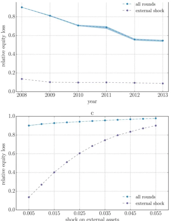
Methodsfor more details). In the top panels ofFig 1we compare the total relative equity lossH
(t) =∑iHi(t) directly due to the initial shock (i.e. at timet= 1) with the one that includes losses generated by the contagion dynamics (i.e. at the convergence of the algorithm), for all the years, and forα= 0.5% and 1%. The overall behaviour resembles the one reported in [37]
obtained using the original DebtRank. However, as already discussed, the relative equity losses observed here are larger by a factor ranging from 1.3 in 2008 to 1.7 in 2013.
We further test this scenario in the bottom panels ofFig 1by focusing on 2008 and 2013 and lettingαvary between 0.5% and 5.5%. The relative equity loss experienced by the system
increases as we increaseα, until it reaches a saturation point. For large enough values ofαmost
of the equity of banks is already wiped out by the initial shock, implying that the amplification due to the contagion dynamics decreases withα. Interestingly, we observe that in 2008 the
amplification pushes relative losses of equity to saturation levels already for values ofαas small
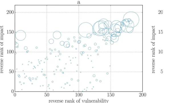
as 0.5%, while in 2013 shock five times larger are needed to reach similar relative losses. As a second scenario, we consider the case in which a single bank at a time is shocked, a shock still being a devaluation of its external assets by a relative amountα, and the experiment
is repeated for each bank. The idea is to decompose the systemic importance of a bank into its impact on the system and into its vulnerability with respect to shocks affecting other banks. We then proceed to define the impact of bankias the relative equity loss of the system when bankiis shocked. Instead we take as a measure of its vulnerability the average ofhi(t) over all
the experiments. We then rank banks in descending order both in terms of impact and in terms of vulnerability and present the results for 2008 and 2013 and forα= 0.5% in form of a
scatter plot inFig 2. We can see that the most dangerous banks, i.e. the banks having the largest impact on the system, are also the most vulnerable ones.
Discussion
Fig 1. Relative equity loss for the system of 183 publicly traded EU banks between 2008 and 2013.All banks are subject to an initial shock consisting in the devaluation of their external assets by a factorα. The violet curves represent the relative equity loss that is directly due to the initial shock, while the blue curves include losses due to the contagion dynamics. Every point is the average over 100 reconstructed networks and the semi-transparent region covers the range between the minimum and maximum across the sample.αis fixed in the top panels and equals to 0.5% (panel a) or 1% (panel b). We see that the amplification effect is reduced from 2008 to 2013. Bottom panels refer to 2008 (panel c) and 2013 (panel d). We see that the relative equity loss saturates for large enough shocks. In 2008 the saturation already occurs for shocks as large as 0.5%.
general, the original DebtRank gives a lower-bound for losses computed with our methodol-ogy, but, for a certain class of shocks, the two algorithms are equivalent on trees. More impor-tantly, we show that the capability of the system to amplify an initial shock depends only on the modulus of largest eigenvalueλ
maxof the matrix of interbank leverages: Whenjλmaxj<1, additional losses induced by subsequent rounds of the dynamics are attenuated over time. In contrast, whenjλ
maxj>1 a small shock will be amplified and cause at least one bank to default. This finding can be important from a regulatory perspective, as one could monitor the evolu-tion ofλ
maxover time to check if the system is entering the unstable regime.
To showcase our algorithm, we apply it to a system composed of 183 European publicly traded banks. We characterise the response of the network to different shock scenarios. Our analysis shows that the amplification of shocks due to interbank contagion consistently decreases from 2008 to 2013, and that in 2008 small shocks are enough for all banks to be sig-nificantly distressed. By performing stress tests in which banks are initially shocked one at a time, we are able to compute both the impact of a single bank on the system and its vulnerabil-ity to shocks initiated by other banks. From a systemic standpoint, it would be desirable that systemic impact and vulnerability were anti-correlated, so that the most dangerous bank are also the most robust, and vice versa. In fact, this does not happen: our analysis shows that the most dangerous banks are also the most vulnerable, meaning that systemic risk is concentrated in a few key players, which should therefore be the objective of effective macroprudential regu-lation policies.
Fig 2. Scatter plot of impact and vulnerability (reverse) rankings in 2008 (panel a) and 2013 (panel b).An initial shock corresponding to a 0.5% devaluation of its assets is applied to one bank at a time, and the experiment is repeated for each bank. The impact of a bank is measured as the relative equity loss experienced by the system when that bank is shocked. The vulnerability of a bank is its relative equity loss averaged over all the experiments. In addition, we average impact and vulnerability across a sample of 100 reconstructed networks. Finally, we build reverse ranking (i.e. in descending order) of both quantities, so that larger values on both axes correspond to more impactful and more vulnerable banks. Bubble size is proportional to the total assets of the corresponding bank. The most dangerous banks are also the most vulnerable.
Methods
Balance sheet basics
A balance sheet summarises the financial position of a bank. It consists of assets, which have a positive economic value (e.g. stocks, bonds, cash), and liabilities, which are obligations to credi-tors (e.g. customers’deposits, other debits). The difference between the value of assets and lia-bilities is called equity, and the following (balance sheet) identity holds: assets = equity + liabilities. A bank is said to be solvent as long as its equity is positive. Once a bank is insolvent, even if it sold the entirety of its assets, it would not be able to repay its debts. As a consequence, we use insolvency as a proxy for default.
Model dynamics
The equation for the evolution of the cumulative relative loss of equityhi(t) = (Ei(0)−Ei(t))/
Ei(0) can be derived from the balance sheet identity. FromEq (2), supposing that (i) external
assets and liabilities do not change, (ii) interbank liabilities are at face value and also do not change, and (iii) interbank assets are marked-to-market,
Eiðtþ1Þ EiðtÞ ¼
X
j2AðtÞ
Aijðtþ1Þ
X
j2Aðt 1Þ
AijðtÞ
¼ X
j2Aðt 1Þ
½Aijðtþ1Þ AijðtÞ
X
j2Aðt 1ÞnAðtÞ
Aijðtþ1Þ;
ð6Þ
where in the second line we have isolated a potential contribution coming from the nodes that were active at timet−1, but became inactive at timet. UsingEq (3), we see that the last term in
Eq (6)vanishes, so that we have:
Eiðtþ1Þ EiðtÞ ¼
X
j2Aðt 1Þ
AijðtÞ
Ejðt 1Þ
EjðtÞ Ejðt 1Þ
h i
¼ X
j2Aðt 1Þ
Aijð0Þ
Ejð0Þ
EjðtÞ Ejðt 1Þ
h i
;
ð7Þ
where in the second line we have recursively appliedEq (3)and usedAij(1) =Aij(0) (only
equi-ties change at timet= 1, assets start to change at timet= 2). We can now define the matrixL~:
~
LijðtÞ ¼ Aijð0Þ
Ejð0Þ if j2Aðt 1Þ
0 if j2=Aðt 1Þ
ð8Þ
8
<
:
and write the equation for the evolution of equity:
Eiðtþ1Þ ¼ max 0; EiðtÞ þ
XN
j¼1
~
LijðtÞ½EjðtÞ Ejðt 1Þ
" #
; ð9Þ
where the max accounts for the fact that once a bank defaults its equity cannot become nega-tive. FromEq (9), it easily follows that:
hiðtþ1Þ ¼ min 1;hiðtÞ þ
XN
j¼1
LijðtÞ½hjðtÞ hjðt 1Þ
" #
; ð10Þ
whereLijðtÞ ¼ ~
leverage matrix, where columns corresponding to banks defaulted up to timet−1 have been set equal to zero. As the equity of defaulted banks does not change anymore after reaching zero, the rows of the leverage matrix corresponding to defaulted banks can be set equal to zero too.
Relation to DebtRank
The original DebtRank [19] has the following dynamics:
hiðtþ1Þ ¼ min 1;hiðtÞ þ
X
A0ðtÞ
WijhjðtÞ
" #
¼ min 1;h iðtÞ þ
X
A0ðtÞ
Wij½hjðtÞ hjðt 1Þ
" #
;
ð11Þ
whereWij= min(1,Λij), andA0(t) = {j:hj(t)>0 andhj(t−1) = 0}, and the last term in the
sec-ond line can be added because it is always equal to zero. Let us note that the definition ofA0(t)
implies a different stopping criterion. In fact, in the original DebtRank nodes propagate shocks only once, immediately after the shock has been received. In our setting, instead, they could propagate shocks until they default. There are two main differences with respect toEq (4a): (i) the summation inEq (11)involves less terms than the summation inEq (4a)sinceA0(t)A
(t)A(t−1) (the set of active nodes becomes smaller and smaller as banks default); (ii)Wij<
Λij, for alliandj. As a consequence,Eq (11)provides a lower bound to relative cumulative losses of equity computed withEq (4a).
In order to understand the role of the network topology, let us focus our attention on a node
r. FromEq (3)we see that a shock can reachronly through the neighboursrborrows from, which in turn can be reached by a shock only through the neighbours they borrow from. In other words, if a single nodesis shocked at some timet, the only possible way forrto experi-ence the effects of such shock (at later times) is that a path fromrtosexists. Let us for a moment suppose that such pathr!i1!i2. . .!ip−1!sis unique (and of lengthp); then
there will be also a unique path leading from any nodeiktos. The shock will propagate to node
ip−1at the timet+ 1, but, if no additional node is shocked, and since no additional paths exist
betweensandip−1, the status of nodeip−1will not change from timet+ 1 to timet+ 2. Similarly the status of nodeip−2will change only at timet+ 2, and so on, until the shock reaches noder
at timet+p. The status of any nodeikon the path will change only at one time step. As a
con-sequence, the result will be the same as if each node were active only when reached for the first time by the shock, as in the original DebtRank. However, this is true only for the nodesrsuch that a unique path connecting them to the only shocked nodesexists. If there are additional paths betweenrandsthe shock will propagate also along those paths, resulting in additional losses at the noder. In particular this is trivially true if the subgraph of nodes reachable (back-wards) from the shocked nodesis a tree. If more than a single node is shocked, and ifris reach-able (backwards) from more than one of them, then, even if the graph is a tree, the
(cumulative) loss experienced byrat the endcouldbe larger than if a stopping criterion à la DebtRank were used. In particular the loss will be larger if the paths are overlapping, while it will be equal if the paths are not overlapping.
Stability properties
notation:
Dhðtþ1Þ ¼ L DhðtÞ ¼ Lt
Dhð1Þ ¼Lthð1Þ; ð12Þ
asΔh(1) =h(1)−h(0), andh(0) = 0. By summing over all the time steps up tot+ 1 one gets:
hðtþ1Þ ¼X tþ1
s¼0
DhðsÞ ¼X tþ1
s¼0
Lshð1Þ: ð13Þ
Δh= 0 is always afixed point of the mapEq (12), and it is stable as long as the modulus of the largest eigenvalueλmaxofΛis smaller than one, meaning that the dynamics will damp
subse-quent propagations of an initial shock over time. In this case the sum inEq (13)will asymptoti-cally converge to:
h1¼ ð1 LÞ 1
hð1Þ: ð14Þ
In contrast, ifjλ
maxj>1,Δh(t) will become increasingly larger, leading to the default of at least one bank, independently from the initial shock.
Eq (12)clearly describes the first stages of the dynamics, up to the first default. Nevertheless, since the reduced leverage matrix does not change between two subsequent defaults,Eq (12)
also holds between one default and the next one, provided thatΛis replaced with the correct reduced leverage matrixΛ(t). As a consequence, the dynamics will remain explosive as long as the modulus ofλ
max(t), the largest eigenvalue ofΛ(t) is larger than one. As more and more banks defaultjλmax(t)jwill eventually become smaller than one, and the dynamics will finally
converge.
It should be noted that modifying the original DebtRank dynamicsEq (11)by allowing banks to propagate shocks as long as their equity is positive would lead to a double-counting of losses. Let us suppose again for simplicity that no banks default and thatW=Λ. Iterating
Eq (11)leads toh(t+ 1) = (I+Λ)th(1), and this quantity is always larger than the one obtained fromEq (13), i.e.Pt
s¼0L
s
hð1Þ.
Data
For our analysis we use the same dataset used in [37]. Information on banks’balance sheets are taken from the Bureau Van Dijk Bankscope database for 183 European banks that were pub-licly traded between 2008 and 2013. From this data source we extract information about: equity, total assets, total liabilities, total interbank assetsA~
iand total interbank liabilitiesL~i. For
details about the handling of missing data, the reader should refer to the aforementioned refer-ence [37].
As mentioned in the main text, the procedure to reconstruct a matrix of interbank assetsAij
develops in two steps: in the first we generate a binary adjacency matrix, which encodes the topology of the network. This is done via a fitness model [41], conveniently modified for
directed networks. A link from bankito bankjis inserted with probabilitypij¼ zxout
i x in j
1þzxout i x
in j, where
thefitness values of each banks are computed asxout i ¼
~
Ai=
P
j ~
Ajandxini ¼ ~
Li=
P
j ~
Lj, and the
parameterzisfixed to attain the desired network density (the number of links in the network divided by the number of possible links). In this paper we have setzso that the density of the network is 5%. We then draw 100 networks according to the probabilitiespij. For each network
algorithm [40]. This consists in the iteration of a map whosen-th step is:
AðijnÞ ¼
Aðijn 1Þ
P
jA
ðn 1Þ
ij ~
Ai
Aðijnþ1Þ ¼
AðijnÞ
P
iA
ðnÞ
ij ~
Li:
At convergence, the above iteration ensures thatP
jAij¼ ~
Aiand
P
iAij¼ ~
Ljfor all banks.
Obviously, one must have thatP
i ~
Ai¼
P
i ~
Li. Since this is not the case for our data, we rescale
liabilities~Liso that the above relation holds.
Acknowledgments
MB, SB, and GC acknowledge support from: FET Project SIMPOL nr. 610704, FET project DOLFINS nr. 640772, and FET IP Project MULTIPLEX nr. 317532. FC acknowledges support of the Economic and Social Research Council (ESRC) in funding the Systemic Risk Centre (ES/ K002309/1). SB acknowledges the Swiss National Fund Professorship grant nr. PP00P1-144689. We thank Stefano Gurciullo and Marco D’Errico for sharing their expertise on the dataset.
Author Contributions
Conceived and designed the experiments: MB SB FC GC. Analyzed the data: MB SB FC GC. Wrote the paper: MB SB FC GC. Developed the conceptual framework: MB FC. Wrote the code and performed the numerics: MB.
References
1. Haldane AG. Why banks failed the stress test; 2009. Speech given at Marcus-Evans Conference on Stress-Testing, London. Available from:http://www.bankofengland.co.uk/archive/documents/ historicpubs/speeches/2009/speech374.pdf
2. Haldane AG. Rethinking Financial Networks; 2009. Speech given at Financial Student Association, Amsterdam. Available from:http://www.bankofengland.co.uk/archive/documents/historicpubs/ speeches/2009/speech386.pdf
3. Trichet JC. Reflections on the nature of monetary policy non-standard measures and finance theory; 2010. Opening address at the ECB Central Banking Conference, Frankfurt. Available from:http://www. ecb.europa.eu/press/key/date/2010/html/sp101118.en.html
4. Cont R, Moussa A, Santos EB. Network Structure and Systemic Risk in Banking Systems. In: Fouque J, J L, editors. Handbook of Systemic Risk. Cambridge University Press; 2010. p. 327–368.
5. Haldane AG, May RM. Systemic risk in banking ecosystems. Nature. 2011; 469(7330):351–355. doi: 10.1038/nature09659PMID:21248842
6. Battiston S, Caldarelli G, Georg CP, May R, Stiglitz J. Complex derivatives. Nature Physics. 2013; 9 (3):123–125. doi:10.1038/nphys2575
7. Caccioli F, Marsili M, Vivo P. Eroding market stability by proliferation of financial instruments. The Euro-pean Physical Journal B: Condensed Matter and Complex Systems. 2009; 71(4):467–479. doi:10. 1140/epjb/e2009-00316-y
8. Caldarelli G. Scale-Free Networks: Complex webs in nature and technology. Oxford University Press; 2007.
9. Boss M, Elsinger H, Summer M, Thurner 4 S. Network topology of the interbank market. Quantitative Finance. 2004; 4(6):677–684. doi:10.1080/14697680400020325
11. Soramäki K, Bech ML, Arnold J, Glass RJ, Beyeler WE. The topology of interbank payment flows. Phy-sica A: Statistical Mechanics and its Applications. 2007; 379(1):317–333. doi:10.1016/j.physa.2006. 11.093
12. Eisenberg L, Noe TH. Systemic risk in financial systems. Management Science. 2001; 47(2):236–249. doi:10.1287/mnsc.47.2.236.9835
13. Elsinger H, Lehar A, Summer M. Risk assessment for banking systems. Management science. 2006; 52(9):1301–1314. doi:10.1287/mnsc.1060.0531
14. Nier E, Yang J, Yorulmazer T, Alentorn A. Network models and financial stability. Journal of Economic Dynamics and Control. 2007; 31(6):2033–2060. doi:10.1016/j.jedc.2007.01.014
15. de Castro Miranda RC, Tabak BM. Contagion Risk within Firm-Bank Bivariate Networks; 2013. Central Bank of Brazil Working Paper No. 322. Available from:http://www.bcb.gov.br/pec/wps/ingl/wps322.pdf 16. Martinez-Jaramillo S, Alexandrova-Kabadjova B, Bravo-Benitez B, Solorzano-Margain JP. An
Empiri-cal Study of the Mexican Banking System’s Network and its Implications for Systemic Risk. Journal of Economic Dynamics and Control. 2014;40:242–265. doi:10.1016/j.jedc.2014.01.009
17. Markose S, Giansante S, Shaghaghi AR.’Too interconnected to fail’financial network of US CDS mar-ket: Topological fragility and systemic risk. Journal of Economic Behavior and Organization. 2012; 83 (3):627–646. doi:10.1016/j.jebo.2012.05.016
18. Montagna M, Lux T. Contagion Risk in the Interbank Market: A Probabilistic Approach to Cope with Incomplete Structural Information; 2014. Kiel Working Paper No. 1937. Available from:http://econstor. eu/bitstream/10419/102271/1/wp-08.pdf
19. Battiston S, Puliga M, Kaushik R, Tasca P, Caldarelli G. DebtRank: Too Central to Fail? Financial Net-works, the FED and Systemic Risk. Scientific Reports. 2012;2:541. Available from:http://dx.doi.org/10. 1038/srep00541
20. Brummitt CD, Sethi R, Watts DJ. Inside Money, Procyclical Leverage, and Banking Catastrophes. PLoS ONE. 2014;9(8):e104219. Available from:http://dx.doi.org/10.1371/journal.pone.0104219 21. Caccioli F, Shrestha M, Moore C, Farmer JD. Stability analysis of financial contagion due to overlapping
portfolios. Journal of Banking & Finance. 2014; 46:233–245. doi:10.1016/j.jbankfin.2014.05.021 22. Caccioli F, Farmer JD, Foti N, Rockmore D. Overlapping portfolios, contagion, and financial stability.
Journal of Economic Dynamics and Control. 2015; 51:50–63. doi:10.1016/j.jedc.2014.09.041 23. Corsi F, Marmi S, Lillo F. When micro prudence increases macro risk: The destabilizing effects of
finan-cial innovation, leverage, and diversification; 2013. Available from:http://ssrn.com/abstract=2278298 24. Bardoscia M, Livan G, Marsili M. Financial instability from local market measures. Journal of Statistical
Mechanics: Theory and Experiment. 2012; 2012(08):P08017. doi:10.1088/1742-5468/2012/08/ P08017
25. Battiston S, Caldarelli G. Systemic Risk in Financial Networks. Journal of Financial Management, Mar-kets and Institutions. 2013; 2:129–154. Available from:http://dx.doi.org/10.12831/75568
26. Roukny T, Bersini H, Pirotte H, Caldarelli G, Battiston S. Default cascades in complex networks: Topol-ogy and systemic risk. Scientific reports. 2013; 3:2759. doi:10.1038/srep02759PMID:24067913 27. Bank of England. A framework for stress testing the UK banking system; 2013. October. Available from:
http://www.bankofengland.co.uk/financialstability/fsc/documents/discussionpaper1013.pdf
28. Basel Committee on Banking Supervision. Global systemically important banks: assessment methodol-ogy and the additional loss absorbency requirement; 2011. November. Available from:http://www.bis. org/publ/bcbs201.pdf
29. Gai P, Kapadia S. Contagion in financial networks. Proceedings of the Royal Society A: Mathematical, Physical and Engineering Sciences. 2010; 466(2120):2401–2423. doi:10.1098/rspa.2009.0410 30. Upper C. Simulation methods to assess the danger of contagion in interbank markets. Journal of
Finan-cial Stability. 2011; 7(3):111–125. doi:10.1016/j.jfs.2010.12.001
31. Caccioli F, Catanach T, Farmer JD. Heterogeneity, correlations and financial contagion. Advances in Complex Systems. 2012; 15(2):1250058. doi:10.1142/S0219525912500580
32. Halaj G, Kok C. Assessing interbank contagion using simulated networks. Computational Management Science. 2013; 10(2-3):157–186. doi:10.1007/s10287-013-0168-4
33. Hurd T, Gleeson J. A framework for analyzing contagion in banking networks; 2011. Available from: http://arxiv.org/abs/1110.4312
34. Battiston S, Delli Gatti D, Gallegati M, Greenwald B, Stiglitz JE. Liaisons dangereuses: Increasing con-nectivity, risk sharing, and systemic risk. Journal of Economic Dynamics and Control. 2012; 36 (8):1121–1141. doi:10.1016/j.jedc.2012.04.001
36. Furfine CH. Interbank exposures: Quantifying the risk of contagion. Journal of Money, Credit and Bank-ing. 2003; 35:111–128. doi:10.1353/mcb.2003.0004
37. Battiston S, Caldarelli G, D’Errico M, Gurciullo S. Leveraging the network: a stress-test framework based on DebtRank; 2015. Available from:http://arxiv.org/abs/1503.00621
38. Cimini G, Squartini T, Garlaschelli D, Gabrielli A. Systemic risk analysis in reconstructed economic and financial networks; 2014. Available from:http://arxiv.org/abs/1411.7613
39. Cimini G, Squartini T, Gabrielli A, Garlaschelli D. Estimating topological properties of weighted net-works from limited information; 2014. Available from:http://arxiv.org/abs/1409.6193
40. Upper C, Worms A. Estimating Bilateral Exposures in the German Interbank Market: Is there a Danger of Contagion? European Economic Review. 2004; 48(4):827–849. doi:10.1016/j.euroecorev.2003.12.009 41. Musmeci N, Battiston S, Caldarelli G, Puliga M, Gabrielli A. Bootstrapping topological properties and