Determination of the optimal periodic maintenance policy under imperfect repair assumption

(1)

Universidade Federal de Minas Gerais Escola de Engenharia

Departamento de Engenharia de Produção

Programa de Pós-Graduação em Engenharia de Produção

Determination of the optimal periodic maintenance

policy under imperfect repair assumption

Maria Luíza Guerra de Toledo [email protected]

Professor: Dra. Marta Afonso Freitas [email protected]

(2)

Abstract

An appropriate maintenance policy is essential to reduce expenses and risks related

to repairable systems failures. The usual assumptions of minimal or perfect repair at

failures are not suitable for many real systems, requiring the application of Imperfect

Repair models. In this work, the classes Arithmetic Reduction of Age and

Arith-metic Reduction of Intensity, proposed by Doyen and Gaudoin (2004) are explored.

Likelihood functions for such models are derived, and the parameters are estimated,

allowing to compute reliability indicators to forecast the future behavior of the failure

process. Under the classic Imperfect Repair virtual age model presented by Kijima et

al. (1988) (particular case of Aithmetic Reduction of Age class), a periodic Preventive

Maintenance policy is proposed, which estimates optimal time intervals for

Preven-tive Maintenance, in order to minimize (prevenPreven-tive and correcPreven-tive) maintenance costs.

Under a dynamic perspective, it is showed how this policy can be improved, using each

failure observation in order to recalculate the optimal time to Preventive Maintenance

for a particular system, considering the effect of the repair action. These policies are

applicable to any Imperfect Repair model. Monte Carlo simulation studies are

imple-mented in order to evaluate the performance of the proposed methods. Those methods

are applied to a real situation regarding the maintenance of engines of off-road trucks

used in a mining company. These results bring valuable information to support

(3)

List of Figures

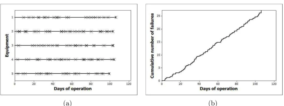
2.1 Example of an off-road truck . . . 5 4.1 (a) Failure times in days of operation for each truck (horizontal lines

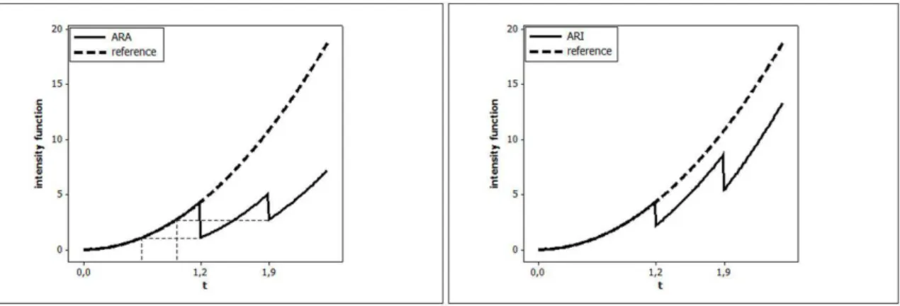
are trucks and “x” are failures); (b) Cumulative number of failures versus days of operation. . . 13 4.2 ARA1 and ARI1 failure intensity functions for PLP intensity function

with β = 3, η = 1, and θ = 0.5, and observed failure times T1 = 1.2

and T2 = 1.9. . . 16

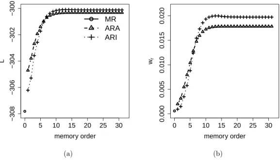
4.3 Criteria values for model selection versus memory order (m), under each fitted model for the trucks data set. Dot, triangles and crosses represent values for MR, ARA and ARI models, respectively. The y -axis in each graph are: (a) Maximum of log-likelihood, and (b) Weight - Eq. 4.7. . . 23 4.4 Estimated intensity functions under the fitted models, considering the

first five failure times for one of the sample trucks. MR, ARA1 and

ARA∞ models are showed on the left, while ARI1 and ARI∞ are on

the right. . . 24 4.5 Estimated reliability functions at T23 = 106.429 days for the trucks

data set under the fitted models. . . 25 5.1 Mean cumulative number of failures versus time for the 193 off-road

engines. . . 29 5.2 Point estimates for the optimal PM periodicity for each generated

sam-ple, assumingCIR/CP M = (a) 1/1.23, (b) 1/5, and (c) 1/15. . . 46 5.3 Estimated functions for the engines data, under MR (dotted lines) and

IR (solid lines): (a)Λ(ˆ t), (b)λˆ(t)and (c) Dˆ(t)(Equation 5.6 6), versus time. . . 48 6.1 Estimated functions for the engines data set using Toledoet al. (2013)

(6)

List of Tables

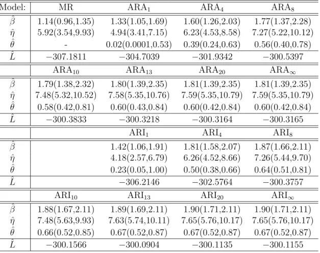
4.1 Point and interval (95%confidence level) estimates for PLP (β,η) and effect of repair (θ) parameters, and the values of the maximum of the log-likelihood function (Lˆ) under each fitted model. . . 22 4.2 Estimated MTTF values at T23 = 106.429 days for the trucks data set

under the fitted models. . . 25 5.1 Simulation Study Results-Performance measures (for point and interval

estimates) for each simulated scenario (assuming MR and PLP withη

(scale) = 16716.53) . . . 44 5.2 Simulated Data under IR assumption- Point and interval estimates

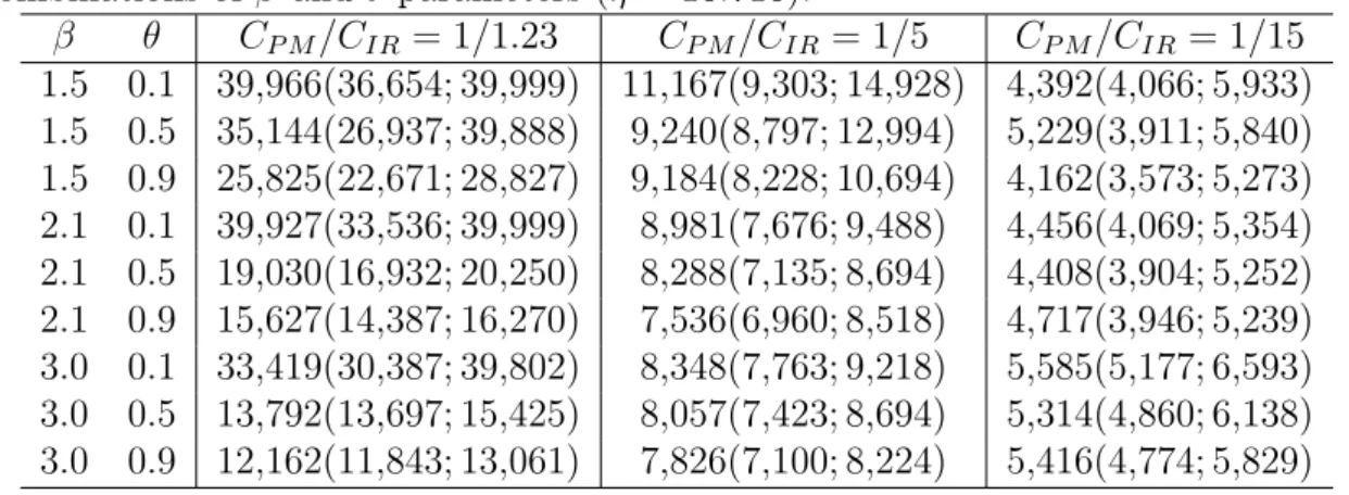
(95% bootstrap CIs with B = 10,000) for the optimal PM periodicity by cost ratio (CIR/CP M) for each sample of n = 193 failure processes generated under different combinations of β and θ parameters (η = 16.716). . . 45 5.3 Off road engines data- Optimal Periodic Maintenance Policy by Cost

Ratio (CIR/CP M), under MR (ˆτM R) and IR (τˆIR) assumptions, and bootstrap (B=10,000) confidence intervals . . . 49 6.1 Estimations for the off-road engines data set, under different values

of costs ratios (CP M/CIR): Optimal PM periodicity (Bˆ−1(CP M/CIR)) based on Toledo et al. (2013) approach; Optimal dyamic PM (τˆV A), and bootstrap (B = 10,000) 95% confidence intervals (values are in hours) . . . 62 6.2 Mean cost per unit time point estimates(1) _{and standard errors}(1,2) _for

(7)

1 Acronyms

ABAO _{As Bad as Old} AGAN _{As Good as New}

ARA _{Arithmetic Reduction of Age} ARI _{Arithmetic Reduction of Intensity} IR _{Imperfect Repair}

MCF _{Mean Cumulative Function} MR _{Minimal Repair}

MTTF _{Mean Time to Failure}

NHPP _{Nonhomogeneous Poisson Process} PLP _{Power Law Process}

PM _{Preventive Maintenance} PR _{Perfect Repair}

(8)

2 Introduction

Since the 80’s, operation and maintenance activities of industrial plants have been recognized as being as important to successful corporative strategies as the product development and manufacturing activities. Operation and maintenance actions play a critical role in a wide range of issues such as security and environmental factors and company profitability levels. It is not difficult to find real-life situations where the environment–safety–profitability triad is present, transforming maintenance into a critical activity. One example is the extracting of oil and gas sector. In 2006, the Petrobras (a brazilian company with business in this sector) announced the discovery of oil reservoir down the sea, below the salt layer. The total depth, i.e., the distance from the sea surface to oil reservoirs below the salt layer can reach 8,000 meters. Consequently, the adoption of appropriate policies for maintenance of the involved equipment is critical, since failures will have a strong impact on the environment, workers safety, and company profitability.

In industries whose production line is composed of complex machines arranged in a serial layout, a single failure may stop the production as a whole, resulting in huge losses and disorders. Similarly, faults in the vehicle fleet carriers can generate costs associated to the displacement of winches and maintenance staff, the rental car to cover the route and even costs related to the loss of cargo. In any of the mentioned cases, the sum of costs arising from the occurrence of failure translates into losses that lead companies to exceed its budget target, resulting in financial distress and damage to its image, and the consequences of the latter are often immeasurable.

For these reasons, the equipment maintenance, once seen as a “necessary evil”, is considered now a strategical activity, indispensable to production, besides being one of the foundations of every industrial activities. The maintenance focus, which was only corrective (ie, after the equipment failure), has became preventive (planned preventative maintenance). Periodicities of interventions have been defined and the maintenance management has evolved further with the use of predictive and inspec-tion techniques. All the tools have been developed in the search of an increased operational reliability.

(9)

- Associação Brasileira de Normas Técnicas, 1994) as the combination of all technical and administrative actions, including supervision, to maintain or replace an item into a state where it can perform a required function. While the Corrective Maintenance is performed after the equipment failure, the Preventive Maintenance (PM) consists of interventions performed in predetermined intervals or according to predefined criteria, aiming to reduce the probability of failure or degradation in the normal operation of a system.

According to Ascher and Feingold (1984), a repairable system (machine, industrial equipment, software, etc.) is the one that, after failing to perform satisfactorily one or more of its functions, can return to its operating condition by some repair (replacement or repair of a component) without needing to replace the system as a whole. Probabilistic and statistical models to analyze and optimize the performance of repairable systems have been widely discussed in the literature. Such models must describe the occurrence of events (failures) over time and the effect of corrective maintenance (repairs). Thus, any study to determine an appropriate PM policy for repairable systems must be based on such models.

In the literature, the most explored assumption about the effect of corrective main-tenance is the Minimal Repair (MR), where it is assumed that each repair action fo-cuses on correcting only the component that originated the failure, leaving the system in the same condition as it was before the failure (As Bad as Old (ABAO)). Under this assumption, the associated failure process can be described by a Nonhomoge-neous Poisson Process (NHPP). According to Muralidharan (2008), in a NHPP, the probability of failure in a small time interval depends only on the age of the system. Thus, the failure intensity function, which provides the instantaneous probability that an event (failure) occurs at time t, conditional on the process history, depends only on t, in the absence of covariates.

(10)

Good as New (AGAN)), and in the present work, we assume that every PM have this effect, so perfect PM will be referred to simply as PM.

The work of Barlow and Hunter (1960) was the driver of a large number of studies that aimed to determine PM policies under MR. Among these, we mention Morimura (1970), Park (1979), Phelps (1981), Barlow and Proschan (1987), Park et al. (2000), and Wang (2002). In particular, Gilardoni and Colosimo (2007) used a Power Law Process (PLP) to model the occurrence of failures, and determined the optimal fre-quency of PM by minimizing a cost function.

The MR assumption seems plausible for systems consisting of many components, each one having its own failure mode, as the repair of the failed component does not change the failure rate of the system. However, in practice, this assumption may not be reasonable for many systems. According to Kijima et al. (1988), for systems composed of only a few vulnerable components, it is more appropriate to consider that the repair brings the state of a failed system to an intermediate level between the completely new and pre-failure. In addition, the mobilization of a maintenance crew to fix a fault often leads to more actions related to system maintenance than those specifically related to the repair. Several authors have studied the behavior of systems subject to this kind of action, called Imperfect Repair (IR).

Brown and Proschan (1983) investigated the failure process assuming that the maintenance action performed after a failure is a perfect repair (AGAN) with proba-bility equal top, and IR with probability equal to1−p. The resulting model is known as B–P Model, and originated several works such as Block et al. (1985), Whitaker and Samaniego (1989), Sheu and Griffith (1992) and Cui et al. (2004).

Kijima et al. (1989) introduced the idea of virtual age of a system, which is a positive function of its real age and its failures history. The virtual age model proposed introduces one parameter, denoted by θ (0≤ θ ≤ 1), which represents the effect of repairs, and includes ABAO and AGAN as special cases (θ =0 and θ = 1, respectively). Doyen and Gaudoin (2004) proposed two classes of IR models. In the first class, the effect of the repair is expressed by a reduction in the failure intensity (ARI model), while in the second, the effect of the repair is expressed by a reduction in the virtual age of the system (ARA model).

(11)

in IR models (Shinet al., 1996; Yanez et al., 2002; Pan and Rigdon, 2009; Doyen and Gaudoin, 2006 and 2011, and Corset et al., 2012), few investigations have been done in the use of such models for determining optimal PM policies, and therefore is the central theme of this work.

2.1 Problem definition

The main motivation for this work was a practical problem in a Brazilian mining company. In the mining sector, the production process is highly dependent on large equipment. To maintain a constant supply of ore to the treatment plant, it is necessary to replace an off-road truck that operates in the transport between the mining front and homogenization cell, as soon as a failure occurs. As it is necessary to keep extra off-road trucks, to act as backups, failures in these systems should be avoided in order to minimize the number of necessary spare trucks, and increase the fleet availability. According to Abranches (2013), in the company unit under study, there are several managers who assist the mining activity, and among them, there is a manager related to the maintenance of large components such as electric motors and diesel engines, and other types of industrial equipment. Diesel engines are mainly used in off-road trucks, which are capable of carrying hundreds of tons of material daily. Figure 2.1 exhibits such a truck. These trucks have a high degree of embedded technology, which enables the use of modern georeferenced systems. These systems make real-time routing of the trucks between various points in the mine, such as mining fronts, the cell homogenization and barren areas disposal.

The reliability of these trucks depends on the reliability of many of its components such as the engine, the weighbridge, the tracking system and the cockpit. The engine is responsible for propelling the truck, while the correct operation of the weighbridge is related to its productivity in cargo transportation. The tracking system is used to determine the routes to be followed between the points of loading and unloading, as well as allowing control of other systems, and the cockpit is related to safety and occupational health of the operator.

(12)

Figure 2.1: Example of an off-road truck

engines. These can be taken from a truck, for maintenance actions, and replaced by another so that the truck can operate again in the shortest possible time. Because of this, when a component is stopped to PM, there is the cost associated to the idle truck that the engine was serving, due to the time for replacement by another in perfect condition.

Each one of these engines goes through a PM program. According to recommenda-tions from the manufacture’s manual, systems must undergo PMs at a predetermined frequency (15,000 hours). However, due to a larger sporadically demand, in practice it is not always possible. Failures can also occur in these engines, even in the ones where PMs are held periodically. In such cases, the failed engine must undergo a corrective maintenance to restore its use conditions.

For a group of engines, data related to their functioning were collected. The accumulated working hours were stored, as well as the number of hours when each PM or failure occurred. As detailed below, statistical analyzes in these data showed that the repair actions taken after failures are neither MR nor perfect repairs. Therefore, the use of an IR model that considers the degree of repair actions is required.

It is of interest to avoid a break in these engines, and consequently to reduce the necessity for corrective maintenance, which has higher cost (on average approximately

(13)

a policy which minimizes the total maintenance cost, i.e., the costs associated to PM and corrective maintenance actions. Thus, it is possible to improve the reliability of these engines, which are essential to the operation of the production process from the mining company.

2.2 Objectives

This work aims at the development of statistical models for the analysis of fail-ure and equipment repairs data, in order to subsidize the elaboration of an optimal maintenance policy. The focus is on situations where the system is subjected to a program of periodic preventive maintenance (assumed here to be perfect) and cor-rective maintenance in the occurrence of failures. However, we work here with the more general assumption of imperfect repair at failures. The goal is to determine the optimal frequency of PMs, where the “optimal” goes in the sense of minimizing the total maintenance cost.

The following specific objectives can be enumerated:

• The preparation of a detailed study about the classes of IR models proposed by Doyen and Gaudoin, 2004 (ARA and ARI models). For such models, we intend to explore:

– The use of maximum likelihood estimation method to obtain estimates for the involved parameters;

– The selection of the best fitted model, considering different memories in each class, using criteria for model selection;

– The prediction of the future failure process of repairable systems using reliability indicators based on such models.

• The determination of a PM policy under IR which specifies the optimal PM frequency;

(14)

• The performance comparison between the two proposed policies in terms of maintenance costs, under different scenarios.

(15)

3 Layout of the text

The core of the text is a collection of three articles dealing with statistical mod-els for IR. The three articles were developed with the following co-authors: Marta Afonso Freitas (Departamento de Engenharia de Produção, UFMG), Enrico Colosimo (Departamento de Estatística, UFMG) and Gustavo Gilardoni (Departamento de Es-tatística, UnB).

The first article considers ARI and ARA classes of models proposed by Doyen and Gaudoin (2004). The estimation in such models is explored and applied to a real dataset. Note that these data do not refer to those described in Section 2.1, but were used at this stage due to the extensive record of failures, allowing us to explore the differences between the studied models. This work is summarized in the first article, entitled “ARA and ARI Imperfect Repair Models: A Case Study in a Brazilian Mining Company”, submitted to the journal Reliability Engineering and System Safety. This article is presented in Section 4.

The second article of this thesis derives a statistical procedure to estimate a peri-odicity PM policy under the following assumptions: (1) perfect repair in PM, and (2) IR after each failure. This policy presents optimal time intervals for PM, in order to minimize the total expected cost with maintenance actions. Its usage is illustrated as a solution to the problem that motivated this work, described in Section 2.1. This article, entitled “Optimal Periodic Maintenance Policy under Imperfect Repair: A Case Study of Off-Road Engines”, submitted to the journal European Journal of Operational Research and currently under revision, is presented in Section 5.

The third and final article in this thesis, presented in Section 6, discusses both the determination and practical implementation of an optimal PM policy under IR. This policy considers the information provided by new failures observed in a repairable system, allowing to recalculate the optimal time for the next PM, based on the effect of the repair performed. The proposed method is also applied as a solution to the problem of the off-road engines. This study comprises the article entitled “Dynamics of the Optimal Maintenance Policy under Imperfect Repair Models”, which is being revised for submission.

(16)

(17)

4 ARA and ARI Imperfect Repair Models: A Case

Study in a Brazilian Mining Company

4.1 Abstract

An appropriate maintenance policy is essential to reduce expenses and risks related to equipment failures. A fundamental aspect to be considered when specifying such policies is to be able to predict the reliability of the systems under study. The usual assumptions of minimal or perfect repair at failures are not appropriate for many real systems, requiring the application of imperfect repair models. In this paper, the classes Arithmetic Reduction of Age and Arithmetic Reduction of Intensity models proposed by Doyen and Gaudoin (2004) are explored. Likelihood functions for such models are derived, assuming Power Law Process and a memory of general order. Based on this, point and interval estimates were obtained for a real dataset involving failures in trucks used by a Brazilian mining company considering models with different memories. Specific statistical measures were used for model selection. Model parameters, namely, shape and scale for Power Law Process, and the efficiency of repair were estimated for the best fitted model. They provided evidences that the trucks tend to fail more frequently over time, justifying the necessity for preventive maintenance, and also, that the repairs after failures tend to leave the equipment in a state between as good as new and as bad as old. The Estimation of model parameters allowed to derive reliability indicators to forecast the future behavior of the failure process. These results are a valuable information for the mining company. They can be used to support decision making regarding preventive maintenance policy.

4.2 Introduction

(18)

et al. (2013). In general, these works are concerned with the study and optimization of PM policies, through the minimization of maintenance cost functions.

These cost functions, and consequently, the resulting PM times, depend on the model and the parameters. In general, these parameters are not known in practice, and, therefore, must be estimated from data. These estimates provide valuable infor-mation about the systems under study, and allow to (1) assess the aging speed and the efficiency of repair actions taken after failures; (2) estimate predictive reliability indicators such as failure intensity and Mean Time to Failure (MTTF) and (3) use these estimates in a PM optimization procedure (Doyen and Gaudoin, 2011). This paper is concerned with the two first issues.

When considering models for repairable systems, a critical point is how to account for the effect of repair actions taken after failures. In this sense, the most explored assumptions are Minimal Repair (MR), which returns the system to the condition just before the failure (ABAO), and Perfect Repair (PR), which leaves the system as if it were new (AGAN). These assumptions were discussed in many works such as Barlow and Hunter (1960), Phelps (1981), Barlow and Proschan (1987), Zhao and Xie (1996), Park et al. (2000), and Wang (2002), among others.

Nevertheless, a more realistic assumption for many systems is the Imperfect Repair (IR) condition. It means that the system returns to an intermediate state between MR and PR. Nowadays some studies have explored this assumption, among them are Kijima et al. (1988), Brown and Proschan (1983), Malik (1979), Shin et al. (1996), Yanez et al. (2002), Pan and Rigdon (2009), and Corset et al. (2012). The former one have proposed the idea of a virtual age model. It is important to emphasize that under MR or PR assumptions, the model parameters are basically those related to the wear-out speed of the systems, while under IR approach, an additional parameter describes the effect of repair actions. Therefore it is necessary to develop an estimation method to take this new parameter into account.

(19)

the calculation of the intensity function. The virtual age model proposed by Kijimaet al. (1988) corresponds to a particular case of these classes, ARA model with memory of order 1, denoted by ARA1.

The present study was conducted in order to investigate the adequacy of ARA and ARI models to a real data set. It was motivated by a situation involving maintenance problems in dump trucks owned by a Brazilian mining company. An unexpected failure in these equipments is extremely costly and harmful due to safety aspects, and also due to operational issues, such as delays in cargo delivery, overtime for employees, unavailability of equipment, and realignment of maintenance resources causing delays in scheduled maintenance on other systems. Each truck is a complex system, so each repair action may involve the replacement or repair of many or only a small fraction of its constituent parts. Thus, assuming MR or PR at failures may result in a simplification that does not correspond to the real condition. This fact motivated the use of IR models in this data set.

Data set consists of failure records in a sample of five trucks from the mining company fleet. Data were collected from July to October 2012, when 129 failures were observed, each one followed by a repair. Figure 4.1 (a) shows events (failures) vs. operation time (in days), where each line corresponds to a sample unit, and each “x” symbol represents a failure time. The data for the five trucks were failure truncated, meaning that the last observation for each one corresponds to a failure time. Visually, no trend in failures over time can be observed from this graph. Figure 4.1 (b) exhibits the mean observed cumulative number of failures. Globally, this curve is neither concave nor convex, so neither improvement nor degradation of the observed equipment can be detected through this visual inspection.

The goal here is to (1) identify which model better fits the data, considering ARA and ARI with different memory values; (2) obtain point and interval parameter es-timates for the best fitted model, specially, for the effect of repair parameter; (3) use these estimates to compute reliability indicators for the trucks, and then, pro-vide information to base the decision-making related to PM policies in the mining company.

(20)

(a) (b)

Figure 4.1: (a) Failure times in days of operation for each truck (horizontal lines are trucks and “x” are failures); (b) Cumulative number of failures versus days of operation.

along with an example for a better understanding of the differences between them. Likelihood functions for these models are presented in Section 4.4. Measures to com-pare the models are also discussed, and predictive reliability indicators are derived. This methodology is then applied to the dump trucks data set, and the results are presented in Section 4.5. Finally, Section 4.6 ends the paper with some concluding remarks.

4.3 ARA and ARI classes of models

Assuming that failures in a repairable system are equivalently defined by the pro-cesses {N(t)}t≥0, or {Ti}i≥1, where N(t) denotes the number of observed failures up

to time t, Ti corresponds to the time elapsed up to the ith failure, and that a re-pair action (with negligible duration) is taken after each failure, the distribution of such processes is completely determined by the failure intensity (or simply intensity) function defined by

ρ(t) = lim

δt→0

P(N(t+δt)−N(t) = 1|ℑt−)

δt , ∀t ≥0 (4.1)

where ℑt− is the minimal filtration defined by the history set of all failure times

occurred beforet. It can be shown (Aalen, 1978) that the Mean Cumulative Function (MCF) of the process is Λ(t) = E[N(t)] =Rt

0 E[ρ(u)]du.

(21)

of failures (ROCOF) function, given by

λ(t) = lim

δt→0

P(N(t+δt)−N(t) = 1)

δt . (4.2)

Under MR assumption, the failure process is a NHPP, andρ(t) =λ(t). A versatile and extensively explored parametric form under this assumption is the PLP, with ROCOF function λ(t) = (β/η)(t/η)β−1 _{and its MCF is given by} _Λ(_t_{) =}Rt

0 λ(u)du = (t/η)β _{(Crow, 1974). Here,}_η _{is a scale parameter, and}_β _{is a shape parameter. When}

β >1,λ(t)increases in t and the system is deteriorating.

Under the IR approach, the model proposed by Kijimaet al. (1988) has the virtual age of a system in time t expressed by

Vt =V(t;N(t);T1,T2, . . . ,TN(t)), (4.3) whereTN(t)denotes the elapsed time since the startup of the system and theN(t)th

failure. Under this model, each repair reduces the virtual age of the system, and the effect of repair is represented by a parameter denoted by θ (0 ≤ θ ≤ 1), including ABAO and AGAN as special cases (θ = 1 and θ= 0, respectively).

In ARA class of models proposed by Doyen and Gaudoin (2004), it is assumed that the system failure intensity at time t (real age) is equal to its ROCOF at time

Vt (virtual age), where Vt ≤ t. Also, between two consecutive failures, its failure in-tensity is horizontally parallel to its ROCOF. ARA models are defined by its memory parameterm, so in ARAm model, it is assumed that the repair reduces the increment in system age since the last m failures, and its failure intensity function is given by

ρARAm(t) = λ(t−(1−θ)

min(m−1,N(t)−1)

X

j=0

θjTN(t)−j). (4.4)

At each repair, the θj _{component in this equation makes older repairs have less} effect on reducing the systems virtual age.

An extreme special case of ARA model, namely ARA1, assumes that the repair

effect is to reduce the increment in system age only by the last failure, while in the other extreme, ARA∞ assumes that each repair reduces the virtual age of the system

(22)

ARI is another class of models proposed by Doyen and Gaudoin (2004), where each repair action reduces not the virtual age, but the failure intensity function of the system. In this class, between two consecutive failures, its failure intensity is vertically parallel to its ROCOF. In ARImmodel, it is assumed that the repair reduces the increment in failure intensity since the last m failures, and its failure intensity function is given by:

ρARIm(t) = λ(t)−(1−θ)

min(m−1,N(t)−1)

X

j=0

θjλ(TN(t)−j). (4.5)

Similarly to ARA, ARI1 and ARI∞ are the extreme special cases of ARI class of

models.

In order to illustrate ARA and ARI models, suppose a repairable system whose failure process has a PLP ROCOF with parameters β = 3,η = 1, and effect of repair parameterθ = 0.5. Suppose that failures are observed at timesT1 = 1.2andT2 = 1.9.

According to Equations 4.4 and 4.5, the failure intensity functions for ARA1and ARI1

models are expressed, respectively, by:

ρARA1(t) =

              

λ(t) = 3t2_, ₀_≤_{t <}₁_.₂

λ(t−0.5×1.2) = 3(t−0.6)2_, ₁_.₂_≤_{t <}₁_.₉

λ(t−0.5×1.9) = 3(t−0.95)2_, ₁_.₉_≤_{t < . . .}

· · · ·

ρARI1(t) =

              

λ(t) = 3t2_, ₀_≤_{t <}₁_.₂

λ(t)−0.5×λ(1.2) = 3t2₋₀_.₅_×₃₍₁_,₂₎2_, ₁_.₂_≤_{t <}₁_.₉

λ(t)−0.5×λ(1.9) = 3t2₋₀_.₅_×₃₍₁_,₉₎2_, ₁_.₉_≤_{t < . . .}

· · · ·

Figure 4.2 exhibits ARA1 (left) and ARI1 (right) failure intensity functions for this

system. It can be observed how the intensity function decreases after failures under each model. AfterT1 = 1.2, for example, while under ARA1 the virtual age decreases

to 0.5×1.2 = 0.6, under ARI1, the intensity function decreases to 0.5×λ(1.2). It

(23)

under ARI model, the intensity function decreases, what explains the models nomen-clature.

Figure 4.2: ARA1 and ARI1 failure intensity functions for PLP intensity function

with β = 3,η = 1, and θ = 0.5, and observed failure times T1 = 1.2 and T2 = 1.9.

4.4 Estimation in ARA and ARI classes of models

In this section, likelihood functions associated to the intensity functions 4.4 and 4.5 are derived. They are used to get Maximum Likelihood (ML) estimators for the parameters. Measures for choosing the best model are also discussed, and finally, reli-ability indicators, such as Relireli-ability function and MTTF for each model are derived.

4.4.1 Parameters estimation: The likelihood functions

Consider k identical repairable systems, k = 1,2, . . ., where the failures occur independently, and assume the following conditions:

• At each failure, a repair action of degree θ is performed. • ni failures are observed in the i−th system, i= 1,2, . . . ,k. • N =Pk

i=1ni is the total number of observed failures in the systems.

• Let Ti,j (i = 1,2, . . . ,k, j = 1,2, . . . ,ni) be random variables representing the failure times for the i−thsystem, recorded as the time since the initial start-up of the system (Ti,1 < Ti,2 < . . . < Ti,ni). For time truncated systems, ni is a

(24)

ti,j denote their observed values (data), and Ti = (Ti,1;Ti,2;. . .;Ti,ni)

t _{be the}

(ni×1)random vector of failure times for the ith system.

• If thei−thsystem is time truncated, it is observed until the predetermined time

t∗

i occurs, and if it is failure truncated, it is observed until the predetermined number of failures ni occurs. So, the last observation time refers to a censor in

t∗

i for time truncated, or a failure inti,ni for failure truncated systems.

• Let µ denote the vector of model parameters, which includes the parameters indexing the ROCOF and the repair efficiency parameter θ. For example, as-suming PLP for the ROCOF, we have µ= (β;η;θ)t_.

A likelihood function for this process must combine the joint probability density of the k systems failure times. Using the failure intensity functions in Equations 4.4 and 4.5, the likelihood functions for ARAm and ARIm models are given, respectively, by:

LARAm(µ) =

= k Y i=1 ni Y j=1

{λ(ti,j −(1−θ)

min(m−1,j−2)

X

p=0

θpti,j−1−p)×

×e−Λ(ti,j−(1−θ)Pminp=0(m−1,j−2)θpti,j−1−p)+Λ(ti,j−1−(1−θ)Pminp=0(m−1,j−2)θpti,j−1−p)_{} ×}

×e−Λ(t∗i−(1−θ)

Pmin(m−1,ni−1)

p=0 θpti,ni−p)+Λ(t_i,ni−(1−θ)Pmin(

m−1,ni−1)

p=0 θpti,ni−p)

and

LARIm(µ) =

= k Y i=1 ni Y j=1

{[λ(ti,j)−(1−θ)

min(m−1,j−2)

X

p=0

θpλ(ti,j−1−p)]×

×e−Λ(ti,j)+Λ(ti,j−1)+(1−θ)[ti,j−ti,j−1]Pminp=0(m−1,j−2)θpλ(ti,j−1−p)_{} ×}

×e−Λ(t∗i)+Λ(ti,ni)+(1−θ)[t∗i−ti,ni]Pmin(

m−1,ni−1)

(25)

where, if the system is failure truncated, t∗

i = ti,ni. These likelihood functions

can then be rewritten assuming a PLP for the ROCOF. So, in order to find the ML estimates βˆ,ηˆandθˆofβ, η, θ respectively, the following log-likelihood functions must be numerically maximized for the ARAm and ARIm classes:

lARAm(µ) =logLARAm(µ) =

= k X i=1 ni !

log(β)−β

k

X

i=1

ni

!

log(η) +

+(β−1)

  k X i=1 ni X j=1

log(ti,j−(1−θ)

min(m−1,j−2)

X

p=0

θpti,j−1−p)

 + + k X i=1 ni X j=1  −

ti,j−(1−θ)Ppmin=0(m−1,j−2)θpti,j−1−p

η

!β

+ ti,j−1−(1−θ)

Pmin(m−1,j−2)

p=0 θpti,j

η + k X i=1  − t∗

i −(1−θ)

Pmin(m−1,ni−1)

p=0 θpti,ni−p

η

!β

+ ti,ni−(1−θ)

Pmin(m−1,ni−1)

p=0 θpti,ni−p

η

!

and

lARIm(µ) =logLARIm(µ) =

= k X i=1 ni !

log(β)−β

k

X

i=1

ni

!

log(η) +

+ k X i=1 ni X j=1 log  t

β−1

i,j −(1−θ)

min(m−1,j−2)

X

p=0

θp_tβ−1

i,j−1−p



+

+η−β

  k X i=1 ni X j=1 

−t

β i,j+t

β

i,j−1+ (1−θ)β[ti,j−ti,j−1]

min(m−1,j−2)

X

p=0

θptβ_i,j−₋1₁₋_p



 

+

+η−β

  k X i=1 

−t∗_iβ +t

β

i,ni + (1−θ)β[t

∗

i −ti,ni]

min(m−1,ni−1)

X

p=0

θptβ_i,n−_i1₋_p



 



(26)

Depending on the number of observed failures for the systems under study, ARA and ARI models can be fitted with different memory values (m). For example, if the maximum number of failure times observed for the systems is 5, m can assume the values 1 to 5, with m = 5 corresponding to m =∞. However, fitting many models to a data set requires model selection, and a basic way to achieve this is through the maximum values of the estimated log-likelihoods, which will be denoted here by

ˆ

L. Since all models explored have the same number of parameters, the comparison usingLˆcorresponds to the one obtained from Akaike Information Criterion (AIC) and Bayesian Information Criterion (BIC) measures (Akaike, 1974 and Schwarz, 1978).

Another useful measure to compare models was proposed by Burnham and Ander-son (2004). It is based on the scaling criteria values,

∆r = ˆLmax−Lˆr, (r= 1, . . . ,R) (4.6) whereLˆmaxis the maximum of theRdifferentLˆvalues, considering thatRdifferent models were fitted. This transformation forces the best model to have ∆ = 0, while the rest of the models have positive values. These values can then be used to calculate weights, based on the normalization of the model likelihoods such that they sum to

1 and can be treated as probabilities,

wr =

exp(−∆r/2)

PR

r=1exp(−∆r/2)

. (4.7)

So, the wr are useful as the “weight of evidence” in favor of model r as being the best model in the set.

After fitting and choosing the best model for the data set under study, reliability indicators can be derived from the estimated parameters. The next section presents some of the indicators that can be derived from models 4.4 and 4.5.

4.4.2 Predictive reliability indicators

In order to forecast for future systems behavior, ARA and ARI intensity functions can be used to compute predictive reliability indicators. Considering that the last observed failure time isTn =tn, it can be of interest the time to next failureTn+1−Tn,

(27)

The following functions can characterize the future behavior of the process and they might be useful for the system engineering manager:

• The reliability function at time Tn=tn is

RTn(t) = P(Tn+1−tn > t|ℑTn) =P(N(tn,tn+t] = 0|ℑTn)

= exp

−

Z tn+t

tn

ρ(u)du

. (4.8)

where tn ≤ u ≤ tn+t < Tn+1. This function express the probability that the

system will work without failure for a given time t after Tn, given all the past history of the failure process.

• The MTTF at timeTn =tn is the mean time to the next failure occurring after

Tn, given by

M T T FTn =E[Tn+1−tn|ℑTn] =

Z ∞

0

RTn(u)du, (4.9)

where RTn is the Equation 4.8.

Replacing the intensity functions 4.4 and 4.5 in Equation 4.8, the reliability func-tions for models ARAm and ARIm are given, respectively, by

RTn,ARAm(t) = exp







−

Z tn+t

tn

λ(u−(1−θ)

min(m−1,n−1)

X

j=0

θjtn−j)du

   = exp   

−Λ(t−(1−θ)

min(m−1,n−1)

X

j=1

θjtn−j)

   × × exp   

Λ(−(1−θ)

min(m−1,n−1)

X

j=1

θjtn−j)







(28)

RTn,ARIm(t) = exp







−

Z tn+t

tn

λ(u)−(1−θ)

min(m−1,n−1)

X

j=0

θjλ(tn−j)du

   = exp   

Λ(tn)−Λ(tn+t) +t(1−θ)

min(m−1,n−1)

X

j=0

θjλ(tn−j)







which, in the particular case of a ROCOF modeled by a PLP, become

RTn,ARAm(t) = exp







− t−(1−θ)

Pmin(m−1,n−1)

j=1 θjtn−j

η

!β   × × exp   

−(1−θ)Pmin(m−1,n−1)

j=1 θjtn−j

η

!β 



(4.10)

and

RTn,ARIm(t) = exp

( tn η β −

tn+t

η β) × × exp   

t(1−θ)

min(m−1,n)−1)

X

j=0

θjβ η

tn−j

η

β−1 





. (4.11)

After using the likelihood functions from Section 4.4.1, the ML estimatesβˆ,ηˆand

ˆ

θ can be replaced in Equations 4.10 and 4.11 and then in MTTF formula 4.9, so that the future behavior of a given system can be predicted. The next section presents the results of this methodology when applied to the dump trucks data set.

4.5 Dump trucks data set revisited

(29)

model. Initially, the purpose is to identify which model provides the best fit to the data. Table 4.1 exhibits the results for MR (θ = 1), ARAm and ARIm with

m = 1,4,8,10,13,20,∞. For the data set under study,m = 31corresponds to m=∞, since the maximum number of failures observed was 31. Other memory values in the interval were also considered, but the results were ommited since they do not add valuable information to our conclusions.

Table 4.1: Point and interval (95% confidence level) estimates for PLP (β, η) and effect of repair (θ) parameters, and the values of the maximum of the log-likelihood function (Lˆ) under each fitted model.

Model: MR ARA1 ARA4 ARA8

ˆ

β 1.14(0.96,1.35) 1.33(1.05,1.69) 1.60(1.26,2.03) 1.77(1.37,2.28) ˆ

η 5.92(3.54,9.93) 4.94(3.41,7.15) 6.23(4.53,8.58) 7.27(5.22,10.12) ˆ

θ - 0.02(0.0001,0.53) 0.39(0.24,0.63) 0.56(0.40,0.78) ˆ

L −307.1811 −304.7039 −301.9342 −300.5397

ARA10 ARA13 ARA20 ARA∞

ˆ

β 1.79(1.38,2.32) 1.80(1.39,2.35) 1.81(1.39,2.35) 1.81(1.39,2.35) ˆ

η 7.48(5.32,10.52) 7.58(5.35,10.76) 7.59(5.35,10.79) 7.59(5.35,10.79) ˆ

θ 0.58(0.42,0.81) 0.60(0.43,0.84) 0.60(0.42,0.84) 0.60(0.42,0.84) ˆ

L −300.3833 −300.3218 −300.3164 −300.3165

ARI1 ARI4 ARI8

ˆ

β 1.42(1.06,1.91) 1.81(1.58,2.07) 1.87(1.66,2.11) ˆ

η 4.18(2.57,6.79) 6.26(4.52,8.66) 7.26(5.44,9.70) ˆ

θ 0.23(0.05,1.00) 0.50(0.38,0.66) 0.64(0.51,0.81) ˆ

L −306.2146 −302.5764 −300.3757

ARI10 ARI13 ARI20 ARI∞

ˆ

β 1.88(1.67,2.11) 1.89(1.69,2.11) 1.90(1.71,2.11) 1.90(1.71,2.11) ˆ

η 7.48(5.63,9.93) 7.63(5.74,10.11) 7.65(5.76,10.17) 7.65(5.76,10.17) ˆ

θ 0.66(0.52,0.85) 0.67(0.52,0.87) 0.67(0.52,0.87) 0.67(0.52,0.87) ˆ

L −300.1566 −300.0904 −300.1135 −300.1155

UsingLˆas the criterion for model selection, it can be observed from Table 4.1 that, for ARA and ARI models, in general, increasing the memory (m value) improves the model adequacy (greater Lˆ). Using a memory value equal or above 8does not make a great difference in the model fit, which can be seen especially in the behavior of Lˆ

(30)

0 5 10 15 20 25 30

−308

−306

−304

−302

−300

memory order

L

^

MR ARA ARI

(a)

0 5 10 15 20 25 30

0.000

0.005

0.010

0.015

0.020

memory order wr

(b)

Figure 4.3: Criteria values for model selection versus memory order (m), under each fitted model for the trucks data set. Dot, triangles and crosses represent values for MR, ARA and ARI models, respectively. They-axis in each graph are: (a) Maximum of log-likelihood, and (b) Weight - Eq. 4.7.

in its favor int the data set. However, in order to simplify the conclusions in this paper, ARI∞ model was used as the best one, since its criteria measures are very similar to the ones obtained for ARI13.

For ARI∞, the estimatedβ parameter was1.90, with95%confidence interval given

by 1.71 to 2.11, indicating that the equipment failure intensity function increases with time. It means that the systems are under intrinsic ageing. The trucks tend to fail more frequently over time, justifying the necessity for PM. Point and interval estimates for the effect of repair parameter θ are 0.67(0.52,0.87). It can be observed that it is significantly different than the two extreme cases ABAO (θ= 1) and AGAN (θ = 0). It means that the repairs after failures tend to leave the equipment in a state between AGAN and ABAO. Any attempt to establish a PM policy for these trucks must take these parameter values into account, as assuming the basic assumptions of MR or PR can lead to serious errors.

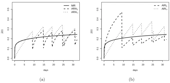
Based on the estimated parameter values from Table 4.1, Figure 4.4 presents the plots of the estimated intensity functions under the extreme models MR, ARA1, ARI1,

(31)

0 5 10 15 20 25 30 0.0 0.1 0.2 0.3 0.4 0.5 days ρ

^(t

)

MR ARA1

ARA∞

(a)

0 5 10 15 20 25 30

0.0 0.1 0.2 0.3 0.4 0.5 days ρ

^(t

)

ARI1

ARI∞

(b)

Figure 4.4: Estimated intensity functions under the fitted models, considering the first five failure times for one of the sample trucks. MR, ARA1 and ARA∞ models

are showed on the left, while ARI1 and ARI∞ are on the right.

Is is remarkable the difference in the behavior of the intensity functions between the worst fitted models (MR, ARA1, and ARI1) and the best one, ARI∞.

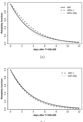
The reliability indicators derived in Section 4.4.2 are an useful tool for providing information about the future behavior of these repairable systems. In order to illus-trate, it is considered one of the five sample trucks, whose last observed failure time is T23 = 106.429 days. We can predict the behavior of the time to next failure (T24),

given the history up to time T23 (ℑT23−). Figure 4.5 shows the reliability functions ˆ

RT23(t) calculated for MR, ARA (Equation 4.10) and ARI (Equation 4.11) models,

using the ML parameters estimates. For the five models considered in the graphs, the reliability function goes from one to zero in12days, that is, the estimated probability of this system work without failure for 12days after T23 = 106.429 is zero, given all

the past of the failure process. While the fitted curve under model ARA∞ is very

close to the best fitted model one (ARI∞), the reliability functions under ARA1 and

MR models tend to overestimate the survival probabilities. This behavior can also be observed in the corresponding MTTF values from Table 4.2. The mean time to the next failure occuring after T23 is 3.1days according to the best fitted model, ARI∞,

(32)

0 2 4 6 8 10 12

0.0

0.2

0.4

0.6

0.8

1.0

days after T=106.429

Reliability function

MR ARA 1 ARA infty

(a)

0 2 4 6 8 10 12

0.0

0.2

0.4

0.6

0.8

1.0

days after T=106.429

Reliability function

ARI 1 ARI infty

(b)

Figure 4.5: Estimated reliability functions at T23= 106.429 days for the trucks data

set under the fitted models.

Table 4.2: Estimated MTTF values at T23 = 106.429 days for the trucks data set

under the fitted models.

Model: MR ARA1 ARA∞ ARI1 ARI∞

3.450 3.719 3.023 3.128 3.144

4.6 Conclusions and final remarks

(33)

applied in order to choose the best fitted model. Estimation of model parameters al-lowed to forecast future behavior of the failure process, through reliability indicators. According to criteria measures for model selection, the best fitted model was ARI∞.

Based on this model, the estimated shape of aging speed (β) parameter was1.90, with

95%confidence interval given by1.71to2.11, and the effect of repair parameterθwas estimated as 0.67(0.52 to0.87). These values give evidences that the trucks tend to fail more frequently over time, and also, that the repairs after failures tend to leave the equipment in a state between AGAN and ABAO. Illustrative predictive reliability indicators for a specific truck in the sample showed that the estimated probability of this system to work without failure for 12 days after the last observed failure time is zero, given all the past of the failure process. Additionally, the estimated MTTF after the last failure indicated that the mean time to the next failure for this system is 3.128 days.

(34)

5 Optimal Periodic Maintenance Policy Under

Im-perfect Repair: A Case Study of Off-Road Engines

5.1 Abstract

In the repairable systems literature one can find a great number of papers that pro-pose maintenance policies under the assumption of minimal repair after each failure (such repair leaves the system in the same condition as it was just before the failure - as bad as old). This paper derives a statistical procedure to estimate the optimal Preventive Maintenance (PM) periodic policy, under the following two assumptions: (1) perfect repair at each PM action (i.e., the system returns to the as good as new state) and (2) imperfect system repair after each failure (the system returns to an intermediate state between as bad as old and as good as new). Models for imperfect repair have already been presented in the literature. However inference procedures for the quantities of interest have not yet been fully studied. In the present paper, statistical methods, including the likelihood function, Monte Carlo simulation, and bootstrap resample methods, are used in order to: (1) estimate the degree of efficiency of repair and (2) obtain the optimal preventive maintenance check points that mini-mize the expected total cost. This study was motivated by a real situation involving off-road engines maintenance.

5.2 Introduction

5.2.1 Motivating situation: Off-road engine maintenance data

(35)

to the global mining industry directly (replacement and corrective repair actions) and indirectly through the inconveniences caused by those failures, such as loss of production, security risks, and reallocation of maintenance resources.

This paper was motivated by a real situation concerning engine failures in off-road trucks used by a Brazilian mining company. This company keeps a database with de-tailed descriptions of all maintenance actions performed on their off-road engines. The data used in this paper are a subset of this database, and include preventive (sched-uled) and corrective (nonsched(sched-uled) maintenance records for a sample of 143 diesel engines. There were 50 Preventive Maintenance (PM) actions during the follow-up period, each assumed to be a perfect repair returning the engine to AGAN condition. Therefore it is fair to say that a new system has been put up into observation just after the PM action.

Consequently, as far as the data analysis is concerned, these 50 PM actions leaded to 50 new systems. The final database consisted of 143+50=193 diesel engines and 208 failure time were recorded. In addition, among the 193 engines, 52 were right censored since their last inspection time corresponded to a system removal for a PM. The perfect repair assumption was verified through a statistical test comparing the 143 original systems to the 50 new ones generated by the PM actions. No evidence of difference between the failures behavior of the two groups was found.

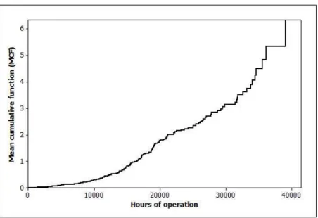
Figure 5.1 plots the mean cumulative number of failures versus time (in hours of operation) for the sample of 193engines. The convex shape of this function indicates that failures tend to occurr more frequently as the system age increases, in other words, the times between failures tend to get shorter with advancing age. This de-teriorating behavior of the engines indicates that PM actions are essential to ensure the reliability of these equipment.

(36)

Figure 5.1: Mean cumulative number of failures versus time for the 193 off-road engines.

5.2.2 Background and literature

In the maintenance literature one can find a great number of papers that propose PM policies under the assumption of Minimal Repair (MR) on failures. In other words, it is assumed that the repair after each failure does not materially change the condition of the system: the repair restores the system to its status immediately before failure (ABAO). Barlow and Hunter (1960) used elementary renewal theory to obtain two types of PM policies, one which is more useful for simple systems (age replacement policy) and another for complex systems (block replacement policy). Related work can be found in Morimura (1970), Phelps (1981), Barlow and Proschan (1987), Park et al. (2000), Wang (2002) and Jaturonnatee et al. (2006).

Gilardoni and Colosimo (2007) considered statistical inference for the optimal PM periodicity under MR using maximum likelihood estimation. More precisely, they applied Barlow and Hunter’s block replacement policy to a real data set concerning failures histories of power transformers. Assuming perfect PM actions (which restore the system to AGAN condition) and MR for failures, the authors came up with a closed form expression for the optimal PM policy, given by check points at every τ

(37)

However, in many practical situations, more realistic notions of repair, intermediate between the two extremes AGAN and ABAO, might be needed. In other words, many repairs actions are more likely to be Imperfect Repairs (IR), and any attempt to elaborate an optimal maintenance policy must take the actual degree of efficiency of these repairs into account. Many models have already been proposed for IR effects (for a review see, for example, Pham and Wang ,1996). Among them are the virtual age models proposed by Kijimaet al. (1988) and Kijima (1989). In particular, Kijima et al. (1988) adapted the block replacement policy by Barlow and Hunter (1960) to the assumption of IR, where the degree of efficiency of the repair is represented by the parameter θ (0≤θ ≤1) and includes ABAO and AGAN as special cases (θ = 1

and θ = 0, respectively). The authors developed a virtual age model to describe the operation over time of a system which is repaired by IRs. But opposed to the MR case developed by Gilardoni and Colosimo (2007), under IR assumption there is no closed form expression to find the optimal PM periodicity. To overcome this difficulty, an approximation procedure was proposed by the authors, but its usage depends on the knowledge of the repair efficiency (θ) and the distribution of the lifetimes of the systems being studied. Numerical examples were provided assuming the particular case of a Gamma distribution, but the model was not statistically studied. More recently, Wu and Zuo (2010) presented a collection of PM models under IR assumption, but statistical estimation for the models parameters was also not discussed.

(38)

(1988) corresponds to the particular case of ARA model with memory 1, namely, ARA1. More recently, Doyen and Gaudoin (2006, 2011) proposed the joint estimation

of aging and maintenance efficiency and also, Pan and Rigdon (2009) and Corset et al. (2012) used Bayesian analysis for the ARA and ARI classes of models, but the focus was not on optimal maintenance policies.

More recently, Remy et al. (2013) presented a case study of technical and eco-nomic optimization of the periodicity of predetermined PM actions carried out on a repairable industrial system from an EDF electric power plant. Using several model selection criteria, the authors came up with the best model, namely [CM ARA∞; PM

AGAN], in other words, corrective maintenance (CM) actions were modeled via an ARA model of order infinity and PM actions modeled as renewals. The parameters associated to the intensity function and efficiency of repair were estimated. Then, using an economic indicator as the optimization criterion, the authors came up with an equation for CT OT, the predictive total maintenace cost. Since CT OT is a random variable, the optimal periodicity w is the value that minimizes the expected value of

CT OT. The search for this optimal value was made through a Monte Carlo procedure whereN = 5×104 _{trajectories were drawn, given a set of fictitious but realistic input}

data.

In the present work we also deal with the estimation of the effect of the repair under a situation where PM actions are modeled as perfect (AGAN) and the corrective actions considered IRs. The main difference of this work with the one of Remy et al. (2013) is that the search for the optimal periodicity was done via an approximation of the mean (cumulative number of failures) function and not by a search for a given set of input data.

5.2.3 The problem

From a modelling point of view, {N(t)}t≥0 (where N(t) denotes the number of

observed failures up to time t) is a stochastic point process, with mean function

Λ(t) =E[N(t)] and failure intensity function

ρ(t) = lim

δt→0

P(N(t+δt)−N(t) = 1|ℑ−_t )

(39)

whereℑ−_t represents the history up to timet(informally, one could think of ℑ−_t as the information provided by the failure times 0< t1 <· · ·< tN(t)< t).

It can be shown (see, e.g. Aalen, 1978) thatΛ(t) = Rt

0 E[ρ(s)]ds .

Before the first maintenance action, the system failure intensity is the rate of occurrence of failures (ROCOF), given by

λ(t) = lim

δt→0

E[N(t+δt)−N(t)]

δt . (5.2)

While ρ(t) depends on the history ℑ−_t, the ROCOF λ(t) is not conditional and hence depends only on t. The ROCOF characterizes the reliability the system would have if it was not maintained.

Under the MP assumption, it is assumed that the effect of maintenance is to leave the system in the same state as it was just before failure. The underlying failure process in this case is a Nonhomogeneous Poisson Process (NHPP), and the failure intensity function ρ(t) equals the ROCOF. In other words, ρ(t) = λ(t),t ≥0.

Under the IR assumption, some functional forms forρ(t)have been proposed in the literature. In particular, for ARA1 model, it can be shown that the failure intensity

is given by (Doyen and Gaudoin, 2004)

ρ(t) =λ(t−(1−θ)TN(t)), (5.3) where Tn is a random variable representing the real age of the system at the nth failure (the elapsed time since the initial start-up of the system) and λ(.) is the ROCOF corresponding to the condition of MR.

If θ = 1, it is assumed that an MR is performed (NHPP). Futhermore, θ = 0

indicates that the system is renewed after each repair and the resulting process is a Renewal Process. Under this model, after each repair the virtual age of the system is reduced by the multiplicative constant 1−θ.

(40)

Λ(τ) =

Z τ

0

E[λ(t−(1−θ)TN(t))]dt. (5.4)

This equation is usually referred to in the literature as the general renewal func-tion, or g-renewal function. Unfortunately, there is no closed form solution for this

equation, except for special cases, such as θ = 1 (MR), orθ = 0 (perfect repair) with the underlying failure times exponentially distributed.

For the general case (0≤θ≤1), a deterministic approximation method for Equa-tion 5.4 was proposed by Kijima et al. (1988). However, applying such an approxi-mation to real systems (which is of great practical interest) is not possible, because this method does not enable estimating the parameters from the failure history data. Later on, Yevkin and Krivtsov (2012) also proposed an approximation for the g-renewal function, but no inference procedure with desirable statistical properties was

proposed.

Although no closed form solution may be obtained for theg-renewal function, this function still can be estimated from the data.

In view of the limitations of the approximations cited above, this paper proposes a procedure to obtain estimators for Equation 5.4 using the observed failure history. The proposed method aims at dealing with the following three issues at the same time, namely: (1)the estimation of the parameters of the intensity function ρ(t)(Equation 5.3), (2) the calculation of an estimator for the mean function Λ(t) (Equation 5.4), and (3) the combination of (1) and (2) to find the optimal PM policy, i.e., to obtain the optimal PM check points (or periodicity τ) that minimize the expected total cost (preventive and corrective maintenance actions) under an IR environment. The method is applied to the failure history of off-road engines.

(41)

presented. Next, it is described how to use these estimates to determine the optimal PM periodicity for a predetermined ratio of costs (CP M/CIR), where CP M and CIR denote the PM and IR actions costs, respectively. Also, a Monte Carlo experiment was run to study the performance of the proposed method. Section 5.6 presents the results of this study, and also illustrates the proposed methodology with simulations. The method is applied to the off-road engines maintenance data and the results are presented in Section 5.7 (point and interval estimates forτ are provided). Conclusions and final comments end the paper in Section 5.8.

5.3 Cost Function and Optimal PM Under an ARA

₁

Model

Consider a system which is subject to failure, and that is put in operation at time

t = 0. Assume the following conditions:

• PM check points are scheduled after every τ units of time;

• at each PM check point, a maintenance of fixed cost CP M is executed, which instantly returns the system to AGAN condition;

• between successive PM check points, an IR of degree θ (0 ≤ θ ≤ 1) is done after each failure, where θ = 1represents an MR (ABAO condition) and θ = 0

a perfect repair (AGAN);

• the expected cost for each IR action is CIR, that is, for each period defined by successive PM check points, the expected total cost is equal to the expected cost per failure times the expected number of failures;

• repair costs and failure times are independent; • repair times are neglected.

Assume that PM is performed everyt units of time. The long run expected main-tenance cost C(t) per unit time for the system is given by (Gilardoni and Colosimo, 2007)

C(τ) = CP M +CIRE[N(τ)]

(42)

Under ARA1 model, E[N(t)] is given by Equation 5.4. The objective here is to

find an optimal PM interval τ which minimizes Equation 5.5. Then, the PM policy that minimizes C(t) is the value τ that satisfies

D(τ) = τ λ(τ)−Λ(τ) = CP M

CIR

. (5.6)

whereλ(τ) = _dτdΛ(τ) is the ROCOF function for the system.

However, under IR assumption no closed form solution can be obtained for the g-renewal function Λ(τ) and, consequently, for Equation 5.6.

In this paper, a procedure to deal jointly with the three following issues is proposed: (1) the estimation of the parameters involved in Equation 5.3, (2) the calculation of an estimator for the mean function Λ(t)(Equation 5.4) from which the ROCOFλ(t)

may be derived, and (3) the combination of (1) and (2) to solve Equation 5.6 for τ, i.e., to find the optimal PM policy.

The individual values of the costs CP M and CIR are not necessary. Instead, only the ratio between them needs to be considered, which simplifies the application in practice.

The first step for finding the optimal PM policy is to estimate the model param-eters. Section 5.4 introduces some additional notation and presents the likelihood function for ARA1 model. In particular, inference procedures for the parameters

involved in Equation 5.3 using a ROCOF modeled by a Power Law Process are pre-sented.

5.4 Parameter Estimation: The Likelihood Function

Consider k identical repairable systems, k = 1,2, . . ., where the failures occur independently. There are basically two ways to observe data from a repairable system. When the data collection stops after a predermined number of failures, the data are said to be failure truncated. On the other hand, when the data collection stops at a predetermined timet, the data are said to be time truncated. The likelihood function is constructed here assuming that among the k observed repairable systems, k1 are

time truncated and k2 are failure truncated, k1,k2 = 1,2, . . . ,k and k1+k2 =k.

(43)

• At each failure, a repair action of degree θ is executed.

• ni failures are observed in theith time truncated system, i= 1,2, . . . ,k1, andn∗j failures are observed in the jth _{failure truncated system,} _j _{= 1}_,₂_{, . . . ,k}

2.

• N =Pk1

i=1ni+

Pk2

j=1n∗j is the total number of observed failures in the systems. • Theith _{time truncated system is observed until the predetermined time}_t∗

i, and the jth _{failure truncated system is observed until the predetermined number of} failures n∗

j occurs.

• Let Ti,l (i = 1,2, . . . ,k1, l = 1,2, . . . ,ni) be random variables representing the

failure times for the ith _{time truncated system, recorded as the time since the} initial start-up of the system (Ti,1 < Ti,2 < . . . < Ti,ni). For time truncated

systems, it is a random number of variables. In addition, let ti,l denote their observed values (data), and Ti = (Ti,1;Ti,2;. . .;Ti,ni)

t _{be the} ₍_n

i×1) random vector of failure times for the ith _{time truncated system.}

• Let Tj,m(j = 1,2, . . . ,k2, m = 1,2, . . . ,n∗j) be random variables representing the failure times for the jth _{failure truncated system, thus being a fixed number of} variables (Tj,1 < Tj,2 < . . . < Tj,n∗

j). Let tj,m denote their observed values. In

addition, let Tj = (Tj,1;Tj,2;. . .;Tj,n∗

j)

t _{be the} ₍_n∗

j ×1)random vector of failure times for the jth _{failure truncated system.}

• LetN(t)be a random variable representing the number of failures in the interval

(0,t].

• Letµdenote the vector of model parameters. It includes the parameters index-ing the process intensity function and the repair efficiency parameter θ.

A likelihood function appropriate to model this process must combine the joint probability density function of the k systems global times, and is given by

L(µ) =

k1

Y

i=1

[fTi|N(t∗i)(ti,1, . . . ,ti,ni|ni)P(N(t

∗

i) =ni)]× k2

Y

j=1

(44)

if k ≥1, k=k1+k2.

The contributions of thek1 time truncated systems and of thek2 failure truncated

systems to the likelihood function are represented by the first and second terms of Equation 5.7, respectively.

As discussed above, the induced intensity function under the ARA1 model is shown

in Equation 5.3. Thus, it is assumed that the failure process has an intensity function which is conditional on the effective maintenance times. For this model, the likelihood function in Equation 5.7 becomes

L(µ) =

k1

Y

i=1

" _n_i Y

l=1

λ(ti,l−(1−θ)ti,l−1)eΛ(θti,l)−Λ(ti,l−(1−θ)ti,l−1)

!

e−Λ(t∗i−(1−θ)ti,ni)

# × × k2 Y i=1   n∗ j Y m=1

λ(tj,m−(1−θ)tj,m−1)eΛ(θtj,m−1)−Λ(tj,m−(1−θ)tj,m−1)



. (5.8)

If the Power Law Process (PLP - Crow, 1974) is used, then the ROCOF function in Equation 5.3 and its corresponding mean function are given, respectively, by

λ(t) = β

η

t η

β−1

, η,β,t >0, (5.9) and

Λ(t) =

Z t

0

ρR(u)du=

t η

β

, (5.10)

Determination of the optimal periodic maintenance policy under imperfect repair assumption

Determination of the optimal periodic maintenance

policy under imperfect repair assumption

Abstract

Contents

List of Figures

List of Tables

1

Acronyms

2

Introduction

2.1

Problem definition

2.2

Objectives

3

Layout of the text

4

ARA and ARI Imperfect Repair Models: A Case

Study in a Brazilian Mining Company

4.1

Abstract

4.2

Introduction

4.3

ARA and ARI classes of models

4.4

Estimation in ARA and ARI classes of models

4.5

Dump trucks data set revisited

4.6

Conclusions and final remarks

5

Optimal Periodic Maintenance Policy Under

Im-perfect Repair: A Case Study of Off-Road Engines

5.1

Abstract

5.2

Introduction

5.3

Cost Function and Optimal PM Under an ARA

Model

5.4

Parameter Estimation: The Likelihood Function