Numerical study of the generation and propagation of ultralow-frequency waves by artificial ionospheric F region modulation at different latitudes

www.ann-geophys.net/34/815/2016/ doi:10.5194/angeo-34-815-2016

© Author(s) 2016. CC Attribution 3.0 License.

Numerical study of the generation and propagation of

ultralow-frequency waves by artificial ionospheric F region

modulation at different latitudes

Xiang Xu, Chen Zhou, Run Shi, Binbin Ni, Zhengyu Zhao, and Yuannong Zhang

Department of Space Physics, School of Electronic Information, Wuhan University, Wuhan 430072, China Correspondence to:Chen Zhou (chenzhou@whu.edu.cn)

Received: 27 January 2016 – Revised: 24 May 2016 – Accepted: 7 September 2016 – Published: 21 September 2016

Abstract.Powerful high-frequency (HF) radio waves can be used to efficiently modify the upper-ionospheric plasmas of the F region. The pressure gradient induced by modulated electron heating at ultralow-frequency (ULF) drives a local oscillating diamagnetic ring current source perpendicular to the ambient magnetic field, which can act as an antenna ra-diating ULF waves. In this paper, utilizing the HF heating model and the model of ULF wave generation and prop-agation, we investigate the effects of both the background ionospheric profiles at different latitudes in the daytime and nighttime ionosphere and the modulation frequency on the process of the HF modulated heating and the subsequent generation and propagation of artificial ULF waves. Firstly, based on a relation among the radiation efficiency of the ring current source, the size of the spatial distribution of the modulated electron temperature and the wavelength of ULF waves, we discuss the possibility of the effects of the background ionospheric parameters and the modulation fre-quency. Then the numerical simulations with both models are performed to demonstrate the prediction. Six different background parameters are used in the simulation, and they are from the International Reference Ionosphere (IRI-2012) model and the neutral atmosphere model (NRLMSISE-00), including the High Frequency Active Auroral Research Pro-gram (HAARP; 62.39◦_{N, 145.15}◦_{W), Wuhan (30.52}◦_N,

114.32◦_{E) and Jicamarca (11.95}◦_{S, 76.87}◦_{W) at 02:00 and}

14:00 LT. A modulation frequency sweep is also used in the simulation. Finally, by analyzing the numerical results, we come to the following conclusions: in the nighttime iono-sphere, the size of the spatial distribution of the modulated electron temperature and the ground magnitude of the mag-netic field of ULF wave are larger, while the propagation loss due to Joule heating is smaller compared to the daytime

iono-sphere; the amplitude of the electron temperature oscillation decreases with latitude in the daytime ionosphere, while it increases with latitude in the nighttime ionosphere; both the electron temperature oscillation amplitude and the ground ULF wave magnitude decreases as the modulation frequency increases; when the electron temperature oscillation is fixed as input, the radiation efficiency of the ring current source is higher in the nighttime ionosphere than in the daytime iono-sphere.

Keywords. Ionosphere (wave propagation) – radio science (ionospheric propagation; waves in plasma)

1 Introduction

waveg-uide, investigating the coupling, transmission, reflection and cutoff of ULF waves and the effects of propagation direction. The shear Alfvén waves and compressional waves propagate independently in the magnetosphere, while in the ionosphere they are coupled through Hall conductivity, which can af-fect the reflection and penetration of ULF waves (Yoshikawa and Itonaga, 1996, 2000; Yoshikawa et al., 1999). Since the ionosphere is not an absolutely perfect conductor itself, ULF waves can penetrate through the ionosphere into neutral at-mosphere then propagate as electromagnetic waves which can be observed on the ground. The 90◦ _{phase rotation of}

magnetic perturbation from the magnetosphere to the atmo-sphere is called Hughes rotation and was thoroughly studied by Hughes (1974) and Hughes and Southwood (1976a, b). Following their previous research, Sciffer and Waters (2002) and Sciffer et al. (2004) presented an analytic solution to the problem of the propagation of ULF waves from the netosphere to the ground in the oblique background mag-netic fields for a thin sheet ionosphere, neutral atmosphere and perfectly conducting ground. In order to investigate the temporal and spatial evolution of ULF waves, Lysak (1997, 1999, 2004) built a numerical model assuming a vertical magnetic field and uniform plasma to study the propagation features of ULF waves in the high-latitude ionosphere with different background parameters and another model includ-ing dipole geometry to analyze magnetosphere–ionosphere coupling by Alfvén waves at midlatitudes by performing a three-dimensional simulation. Also, a new model featuring finite ionospheric conductivity and capable of calculating the ground magnetic field of ULF waves is developed by Lysak et al. (2013) to study the ionospheric Alfvén resonator (IAR) in a dipolar magnetosphere.

Apart from research on the propagation of naturally ex-cited ULF waves, the generation of ULF waves by iono-spheric modulated heating is considered a physical problem of great importance and interest as well. A strong horizon-tal electric current driven by an atmospheric dynamo electric field and a magnetospheric electric field flows in the D or E region of the polar ionosphere, which is called the auro-ral electrojet. Similarly, the equatorial electrojet flows in the lower equatorial ionosphere, which is associated with Cowl-ing conductivity and a tidal electric field. Modulated heatCowl-ing of the lower-ionospheric region where these currents flow with powerful high-frequency (HF) pump waves makes the ionospheric conductivity of the region change periodically, which in turn modulates the preexisting currents in the heated area (Moore, 2007). In the meantime, these oscillating cur-rents form an electric dipole antenna radiating low-frequency waves in the ionosphere. This hypothesis was first suggested by Willis and Davis (1973) and was then proved when artifi-cially excited low-frequency signals were detected in an ex-periment for the first time (Getmantsev et al., 1974). A series of experiments of generating low-frequency waves follow-ing this mechanism were carried out at the European Inco-herent Scatter Scientific Association (EISCAT) and the High

Frequency Active Auroral Research Program (HAARP; Co-hen et al., 2012; Agrawal and Moore, 2012; Moore et al., 2007; Ferraro et al., 1984; Papadopoulos et al., 2003), and this mechanism was named PEJ (polar electrojet) (Stubbe and Kopka, 1977; Barr et al., 1991). The method of arti-ficially generating low-frequency waves by modulating the lower ionosphere is completely dependent on the existence of quasi-stationary ionospheric currents, which to some extent limits the location of the heating facility to the high and equa-torial latitudes and also makes the generation of ULF waves more unpredictable (Papadopoulos et al., 2011b). Moreover, some experimental observations such as ULF artificial ex-cited signals at frequencies of 3.0, 5.0 and 6.25 Hz at Arecibo in 1985 still cannot be explained by classic ionospheric cur-rent modulation mechanism (Ganguly, 1986), which makes it necessary to develop new theories and experimental meth-ods.

In a series of experiments conducted from 2009 to 2010 at HAARP, artificial ULF and lower ELF signals generated by the modulated heating ionospheric F region in the ab-sence of electrojets were received on the ground far away from the heating facility, and the dependence on the heating conditions differs from the low-frequency waves generated by modulating the ionospheric currents (Papadopoulos et al., 2011a, b; Eliasson and Papadopoulos, 2012). This artificial generation of ULF waves relates to the oscillating diamag-netic drift current in the upper ionosphere due to the mod-ulated heating, which is based on the ICD (ionospheric cur-rent drive) theory proposed by Papadopoulos et al. (2007). By modifying the model developed by Lysak (1997), Pa-padopoulos et al. (2011b) built a new model to study the ICD in the polar ionosphere by F region heating in cylindrical ge-ometry. Eliasson et al. (2012) performed a theoretical and numerical study of the ICD based on a numerical model of the generation and propagation of ULF and ELF waves. The simulation results agree with the HAARP experimental mea-surements. Utilizing the ICD method, similar experiments conducted at SURA also received artificially generated ULF waves by modulated heating the F region. A comprehensive investigation of ULF wave properties and their dependence on modulation frequencies, polarization, beam inclination, receiving location and the geomagnetic activity was carried out by Kotik et al. (2013, 2015).

ionospheric parameters and the modulation frequency, based on a relation among the radiation efficiency of the ring cur-rent source, the size of the spatial distribution of the modu-lated electron temperature and the wavelength of ULF waves; secondly, we run the simulation with the HF heating model to investigate the electron temperature response to the mod-ulated heating under different ionospheric conditions with a modulation frequency sweep; thirdly, we run the simulation with the model of ULF wave generation and propagation in the same way to study the radiation efficiency of the ring cur-rent source, the propagation loss and the ground ULF wave magnitude. In Sect. 4, conclusions based on the simulation results and the corresponding analysis are summarized.

2 Numerical model

2.1 Mechanism of artificial generation of ULF waves in ionospheric F region

The radial electron pressure gradient caused by the HF heat-ing in ionospheric F region can drive a local diamagnetic rheat-ing current perpendicular to the ambient magnetic field given by

J_⊥=B0× ∇pe

|B_0|2 , (1)

whereB0is the background magnetic field and∇pe is the

electron pressure gradient in the heated F region (Spitze, 1967). When the HF pump wave is amplitude modulated with the oscillation frequency f in the ULF band, the ring current will oscillate with the same frequency. The empiri-cal evidence of the modification of the F region reveals that the change in electron temperature is larger than the elec-tron density and that the response time of the elecelec-tron den-sity to the HF heating is much longer than that of the electron temperature (Robinson, 1989; Hansen et al., 1992a). There-fore, the electron pressure gradient mainly originates from the electron temperature gradient due to HF heating, and the pressure gradient is given by

∇pe=nekB∇Te, (2)

wherene is the electron density,kB is the Boltzmann

con-stant andT_eis the electron temperature. The oscillatory ring current can be expressed as

J_⊥=nekB

B0× ∇Te

|B0|2

exp(i2πf t ) . (3)

The ring current integrated over the heated volume will cre-ate an oscillating magnetic dipole moment parallel to the am-bient magnetic field, acting as a virtual antenna which ra-diates ULF waves at the modulation frequency in the iono-sphere. Some of ULF waves will penetrate into the Earth– ionosphere waveguide and will be received on the ground.

2.2 HF heating model

The plasma transport model for the F region ionospheric heating model can be described as follows (Bernhardt and Duncan, 1982; Shoucri et al., 1984; Hansen et al., 1992b):

n_ev_{e= −}D

(

∂

∂s[nekB(Te+Ti)]+

X

α

mαnαgk

)

(4)

∂ne

∂s +

∂ (neve)

∂s =Qe−βene (5)

3 2kB

ne ∂Te

∂t +neve ∂Te

∂s

+kBneTe ∂ve

∂s

= ∂

∂s

Ke ∂T_e

∂s

+SHF+S0−Le, (6)

with the subscriptαdenoting electron (e) and ions (i),nαand mα the number density and mass of electron and ions,

re-spectively,TeandTithe electron and ion temperature,kBthe

Boltzmann constant, _∂s∂ the directional derivative along the ambient geomagnetic field,ve=ve·B0/B0the field-aligned

flow velocity, andg_k=g_·B0/B0 the projection of gravity

acceleration along the field line.

Equation (4) is the steady-momentum equation under the assumption of ambipolar diffusion and quasi-neutrality, and electron inertia can be neglected for the time- and space scales under consideration. The diffusion coefficientDcan be expressed as (Hinkel et al., 1992)

D₌ 1

meυen+MIυIN

, M_Iυ_IN=P 1

i

(ni/ne) /miυin

, (7)

with the ionic species indexidesignating the ions involved in our simulation domain, i.e., O+_{, O}+

2 and NO+.υenandυin

are electron–neutral and ion–neutral collisional rates, respec-tively, both of which are calculated from Banks and Kocharts (1973) and Schunk and Nagy (1978).

Equation (5) is the continuity equation along the direc-tion of the geomagnetic field line for ionospheric electrons, whereQ_eis the local ionization source term producing the equilibrium density profile without the HF heating andβ_eis the electron recombination rate.β_eis given by (Hinkel et al., 1992; Schunk and Walker, 1973)

βe=k1nNO++k2nO+

2, (8)

with k₁₌4.2_×10−7(300/T_e)0.85cm3s−1 _{and k}

2=1.6×

10−7(300/T_e)0.55cm3s−1_{. The ion densities of O}+_{, O}+ 2 and

NO+ are obtained and updated according to the impor-tant photochemical equilibrium with the dissociative reaction rates and the source term of ion production rates dependent upon the background densities of neutrals, electron and ions (Park and Banks, 1974; Schunk and Walker, 1973; Schunk and Nagy, 1980; Hinkel et al., 1992).Qe is calculated from

ionospheric density profiles (Shoucri et al., 1984), and it is used as a constant during our simulation.

Equation (6) is the electron energy conservation equation along the geomagnetic field line, which includes the effects of convection and pressure flux and heat conduction. Also note that our simulation is based on the assumption that ion temperatures of O+, O+₂ and NO+and neutral temperatures of N2, O2, O and He are the same and the temperature

re-mains invariant during the simulation.

Keis the parallel coefficient of thermal conductivity which

takes the form of (Banks and Kocharts, 1973)

K_e=

7.75×105T_e2.5

1₊3.22_×104 T_e2/ne P n

NnhQni

eV cm−1s−1K−1, (9)

withNn being the densities of neutrals andhQni the cross

section of the mean neutral–electron momentum transfer, which is calculated from Schunk and Nagy (1978).

L_eis the rate of electron cooling, the physical mechanism of which mainly contains the translational electron–neutral interactions, the rotational and vibrational excitation of N2

and O2, the fine structure excitation of O, and the electronic

excitation of O and O2. The expression ofLecan be found in

Schunk and Nagy (1978).

S0 represents the steady-state source term in the absence

of the heating and can be estimated by Eqs. (4) and (6) by

∂

∂t =0 andSHF=0, which takes the form of S0=Le0−

∂

∂s

Ke0 ∂T_e0

∂s

+3

2kBne0ve0

∂T_e0

∂s

+kBne0Te0 ∂ve0

∂s . (10)

The terms in Eq. (10) with an extra subscript “0” denote the value att₌0 in our simulation, which is exactly calculated from the initial background profiles.S0is also kept invariant

during our simulation likeQ_e. The profile ofS₀used in the simulation is shown in Fig. 6a.

S_HF is the energy absorption from heating waves. Since only thermal process is taken into account, S_HF provides the external heating source for ionospheric changes. For the F region, the heating source term SHFincludes both ohmic

loss and anomalous loss due to the nonlinear wave–wave in-teraction and wave–particle inin-teraction (Meltz et al., 1974; Perkins et al., 1974). The absorption of HF pump power can be expressed as (Shoucri et al., 1984; Gustavsson et al., 2010)

SHF=

1 2Re

E∗_±(z)_·σ_±(z)_·E_±(z)

=1

2σ±|E±(z)|

2_{, (11)}

withE_±(z)being the HF wave electric field,σ_±(z)the elec-tric conductivity tensor, and the subscript “₊” and “₋” repre-senting the right-hand circularly polarized O mode and left-hand circularly polarized X mode, respectively.

The wave field at altitude ofzis calculated as (Shoucri et al., 1984; Gustavsson et al., 2010)

E_±(z)₌

E (z0)

z0 z

ε_±(z0) ε_±(z)

0.25

exp

 ik0

z

Z

z0

N_±(z)dz

 , (12)

withz0 being the bottom altitude of the ionosphere,ε±(z)

the ionospheric dielectric tensor,k0the vacuum wave number

andN_±(z)the ionospheric refractive index expressed as

N_±(z)₌µ_±(z)₊iχ_±(z) . (13)

The real partµ_±(z)and the imaginary partχ_±(z)are related toσ_±(z)andε_±(z)by

N_±2(z)₌(µ_±(z)₊iχ_±(z))2₌ε_±(z)

+i (4π/ω)σ_±(z) , (14)

and the exact expression ofσ_±(z)andε_±(z)can be found in Shoucri et al. (1984).

If ohmic heating is considered as the only mechanism when calculating the absorption of HF pump power by the ionosphere, the energy deposition of the ionosphere when the X mode is used as the pump wave is approximately 4 times larger than that of the O mode (Löfås et al., 2009). This is be-cause the absorption of HF power is dependent on the imagi-nary part of the refractive indexN_±(z)according to Eqs. (12) and (13), andχ₋(z)of the X mode is larger thanχ₊(z)of the O mode. However, near the O mode reflection point of the F2 peak, huge anomalous absorption can be induced by para-metric instability and thermal self-focusing instability when the O mode wave is used as the pump wave, which usually brings about much larger density and temperature enhance-ment than ohmic heating (Perkins and Valeo, 1974; Gure-vich, 1986; Istomin and Leyser, 1997; Kuo, 2015).

In order to achieve a better HF heating effect, the pump wave of the O mode is utilized in our simulation and the fre-quency of the HF wave is adjusted so that the reflection point is near the F2 peak. At the reflection point in our simula-tion, the absorption of HF power is calculated as (Meltz et al., 1974; Perkins and Valeo, 1974)

SHFmax=Sohmic+Sanom= ε0

2

ω_pe2υ_e1

ω₀2

!

E₀2

+16

_n

eTe ω₀

υ_e22

_E

0 E_t

4

, (15)

withS_ohmic being ohmic loss,S_anom the anomalous absorp-tion caused by collisional and Landau damping (Perkins et al., 1974),ε₀ the vacuum dielectric constant,ω_pethe elec-tron plasma frequency at the reflection point, andω0the

fre-quency of the pump wave. The electron collisional frefre-quency inSohmicis calculated as

withυ_ei being the electron–ion collisional frequency at the reflection point; it is derived from Banks and Kocharts (1973) and Schunk and Nagy (1978), while the exact expression of

υ_e2inS_anomcan be found in Perkins et al. (1974). The peak electric field amplitudeE0is estimated by an empirical

for-mula:

E0=

√ 30ERP

z , (17)

with ERP the effective radiated power as a input parameter thus the propagation loss of the HF pump wave is not taken into account. The threshold field value E_t for inducing the anomalous absorption is calculated from Kuo (2015). For simplification of the calculation, we adopt a 2-D Gaussian absorption model taking the form of

SHF=SHFmaxexp

−(x₋xr)2/σx2−(z−zr)2/σz2

, (18)

withS_HFmaxbeing the HF power absorption at the reflection point calculated by Eq. (14), (x_r,z_r), the coordinate of the reflection point in our simulation domain; σx the

horizon-tal half-width; and σz the vertical half-width. According to

the artificial generation of ULF waves in ionospheric F re-gion experiment conducted at HAARP and SURA (Kotik and Ryabov, 2012; Papadopoulos et al., 2011b), the source term

SHFis modulated by ULF square waves with 50 % duty cycle

in our simulation.

2.3 Model of ULF wave generation and propagation In our simulation, the generation model of ULF waves pro-posed by Eliasson et al. (2012) is used to calculate the fol-lowing propagation of ULF waves excited by modulated HF heating. The model is built under the following assumption: firstly, the frequency of the artificially generated ULF wave is far less than the electron cyclotron frequency; secondly, O+ is considered as the only ion dominating the propaga-tion of the plasma wave and the condipropaga-tion of quasi-neutrality

n0=ni=nefor ion and electron number densities is

satis-fied; thirdly, the electron–neutral and ion–neutral collisions are the main collision mechanism when calculating the wave dynamics.

In the ionosphere, the propagation of artificially generated ULF waves is calculated by the following equations:

∂E

∂t = −

υin+ ωci ωce

υen

E₊v_A2H1[∇ ×(∇ ×A)]

− c

2

ω2_peH2[∇ ×(∇ ×E)]+S (19)

∂A

∂t = −E (20)

B_{= ∇ ×}A (21)

S₌kB e

H_3∇δT_e−∂∇δTe ∂t

, (22)

withE being the electric field,B the magnetic field,Athe vector potential introduced by Eq. (20),E_{= ∇}ϕ₋∂_∂tA with the gaugeϕ₌0,cthe speed of light,ωpe=

q

e2_n 0

ε0me the elec-tron plasma frequency,v2_A= B

2 0

µ0n0mi the Alfvén speed,ethe electron charge,n0the number density of electron andµ0the

permeability of free space.

H₁,H₂andH₃are the background parameter matrices tak-ing the form of the followtak-ing expressions:

H1= 

     

υinυen+ωciωcecos2θ ωciωce

(υinωce−υenωci)cosθ ωciωce −

cosθsinθ (υenωci−υinωce)cosθ

ωciωce

υinυen+ωciωce ωciωce

(υinωce−υenωci)sinθ ωciωce

−cosθsinθ (υenωci−υinωce)sinθ ωciωce

υinυen+ωciωcesin2θ ωciωce



     

(23)

H2=

" _υ

en ωcecosθ 0

−ωcecosθ υen ωcesinθ

0 ₋ωcesinθ υen

#

(24)

H3=

"

−υin ωcicosθ 0

−ωcicosθ −υin ωcisinθ

0 ₋ωcisinθ −υin

#

, (25)

withωce=

q

eB0

me and ωci=

q

eB0

mi being the ion and elec-tron cycloelec-tron frequencies, θ the dip angle of the ambient geomagnetic field, andυenandυinthe electron–neutral and

ion–neutral collisional rates, respectively, both of which can be calculated according to Banks and Kocharts (1973) and Schunk and Nagy (1978) as in the HF heating model.

In this model, the modulated HF heating effect is estimated by Eq. (21), in whichδT_eis the electron temperature devia-tion from the background value. When the geomagnetic field is assumed to be vertical,δT_eis calculated as

δTe=δTemaxsin(ωt )exp

"

−(x−xr)

2

D_x2 −

(z₋zr)2 D2_z

#

, (26)

withδTemaxbeing the oscillation amplitude of the electron

temperature,ωthe modulation frequency of HF heating, and

Dx andDz the half-width of the spatial distribution of the δTein the horizontal and vertical direction, respectively. Note

that Eq. (17) and Eq. (25) are similar in form yet their physi-cal meanings are completely different. According to Eliasson et al. (2012), the term ∂∇δTe

∂t mainly generates the waves of

non-propagating modes which are not studied in this paper. In the meantime, the magnetosonic wave is directly excited by the diamagnetic ring current due to the perpendicular elec-tron temperature pressure gradient, while the Alfvén wave is generated by mode conversion from the magnetosonic wave through Hall conductivity. Thus, in our simulation, only the

ycomponent of Eq. (21) is considered, and it is expressed as

SULF= kBωci

e

sinθ∂δTe ∂z −cosθ

∂δTe ∂x

At the boundary between the ionosphere and atmosphere, the boundary condition proposed by Eliasson et al. (2012) is ap-plied. Also, the electromagnetic perturbation in the neutral atmosphere is estimated by analytic expression, and the in-versely spatial Fourier transform is applied to obtain the real space wave field (Eliasson and Papadopoulos, 2009; Eliasson et al., 2012).

2.4 Parameter setting in numerical simulation

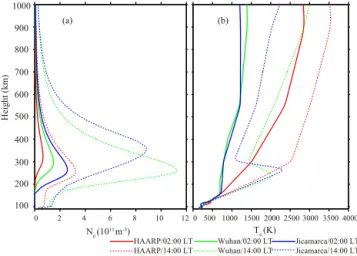
In this paper, simulations with both models introduced pre-viously in Sects. 2.2 and 2.3 are conducted in a two-dimensional computational domain, with x as the horizon-tal direction andzas the vertical direction. The background profiles used in the simulation are one-dimensional functions with height in zdirection and remain constant in x direc-tion. It should be noted that the HF heating model and the ULF wave generation and propagation model share the same background profiles in this paper. In our simulation with both models, HAARP (62.39◦N, 145.15◦W), Wuhan (30.52◦N, 114.32◦E) and Jicamarca (11.95◦S, 76.87◦W) are chosen as the locations of the HF heater. The according ionospheric and atmospheric background profiles are given by the In-ternational Reference Ionosphere (IRI-2012) model and the neutral atmosphere model (NRLMSISE-00). The profiles in-clude the number densities of electron, O+_{, O}+

2, NO+, N2,

O2, O and He, the temperatures of electron, ions and neutrals,

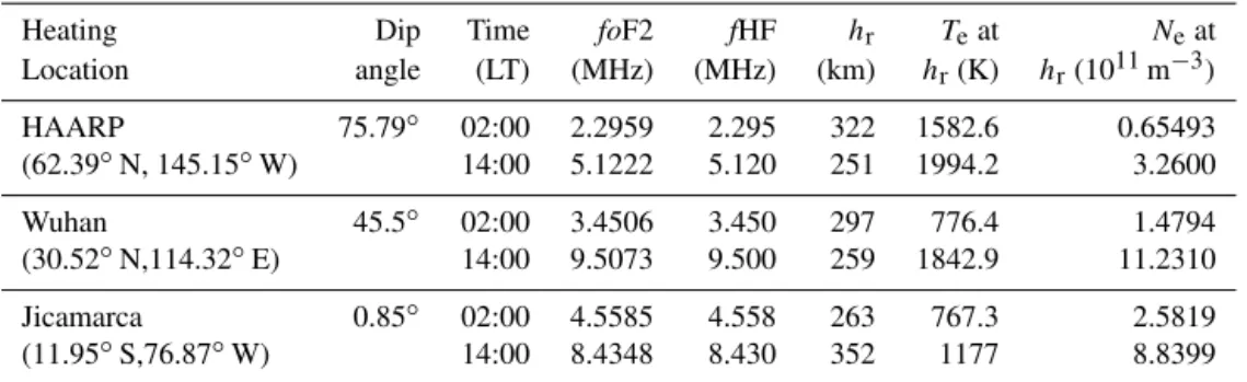
and the dip angleθof the geomagnetic field. The simulation time is set to 02:00 and 14:00 LT, 10 March 2006, to study the effect of the daytime and nighttime ionosphere. The intensity of the background geomagnetic field is set to be 4.0_×105T. The heating parameters for the modulated HF heating are listed in the Table 1, includingfoF2, the electron plasma fre-quency at the peak of the F2 layer; f_HF, the frequency of pump wave;hrthe reflection height of the pump wave; the

electron temperature,Te; and the number density,Ne, athr.

Figure 1 shows the electron density and temperature profiles against height from 90 to 1000 km in the ionosphere used in the simulation.

Now we introduce the setting of the simulation domain. In the simulation with the HF heating model, the spatial grid size in thexandzdirection is 1.0 km, and the time resolution is 1.0_×10−3_{s. The spatial range is from}

−100 to 100 km in the x direction and from 180 to 400 km in the z direc-tion. In the simulation with the wave generation and propa-gation model, the spatial grid size in thexandzdirection is 10.0 km, and the time resolution is 1.0_×10−4s. The spatial range is from₋1000 to 1000 km in thexdirection and from 0 to 1000 km in thezdirection, with the ionosphere from 90 to 1000 km and neutral atmosphere from 0 to 90 km.

0 2 4 6 8 10 12

N_e (1011_m-3₎

(a)

0 500 1000 1500 2000 2500 3000 3500 4000 100

200 300 400 500 600 700 800 900 1000

Height (km)

HAARP/02:00 LT HAARP/14:00 LT

Wuhan/02:00 LT Wuhan/14:00 LT

Jicamarca/02:00 LT Jicamarca/14:00 LT Te (K)

(b)

Figure 1.The background ionospheric electron density and temper-ature profile used in our numerical simulation.

3 Simulation results and discussion

3.1 ULF wave generation and ring current radiation source

According to the physical mechanism of the generation of ULF waves in the ionospheric F region, a diamagnetic ring current source of ULF radiation is driven by the modulated HF heating, which is of crucial importance in the whole wave generation process. So, the relation between the wave gen-eration and the source of ULF radiation due to HF heating should be qualitatively discussed before presenting the sim-ulation results.

Since in the simulation with the model of ULF wave gen-eration and propagation, the electron temperature response to HF heating is estimated with Eq. (25), it is natural that both the amplitude of the electron temperature oscillation and the spatial distribution of theδTeare expected to affect the

gen-eration of ULF waves. An analytical mathematical deduc-tion by Vartanyan (2015) based on Eqs. (18) and (19) has re-vealed the relation between the horizontal half-width of the spatial distribution of theδTeand the radiation efficiency of

Table 1.Heating parameters used in the model.

Heating Dip Time foF2 fHF hr Teat Neat

Location angle (LT) (MHz) (MHz) (km) hr(K) hr(1011m−3)

HAARP 75.79◦ 02:00 2.2959 2.295 322 1582.6 0.65493

(62.39◦N, 145.15◦W) 14:00 5.1222 5.120 251 1994.2 3.2600

Wuhan 45.5◦ 02:00 3.4506 3.450 297 776.4 1.4794

(30.52◦N,114.32◦E) 14:00 9.5073 9.500 259 1842.9 11.2310

Jicamarca 0.85◦ 02:00 4.5585 4.558 263 767.3 2.5819

(11.95◦S,76.87◦W) 14:00 8.4348 8.430 352 1177 8.8399

the shape of the distribution ofδTeafter simplification, which

can be achieved by solving Eq. (27): 1

v2_A ∂2Ay

∂t2 = ∂2Ay

∂x2 + k_Bω_ci

ev2_A ∂δT_e

∂x . (28)

The source termδT_ecan be estimated by Eq. (25) as well but withz₌0. Using the method of the Green function and sim-ply considering the far-field magnitude of the ULF radiation (x_≫Dx), the solution to this equation can be expressed as

Ay₌

√_π

2

ωcikBδTemaxDx

ev2_A

exp

−1 4k

2_D2 x

sin(i (kx₋ωt )) , (29)

withkbeing the wave number of the ULF wave andAy

des-ignating the ground far-field magnitude of the ULF radiation. After substituting k withk₌2π_λ, in which λ is the wave-length of the ULF wave, we can obtain the relation among

A_y

,λandD_x, which takes the form of

Ay

∝exp

− π

2

λ2_/D2 x

. (30)

Eq. (29) indicates that the ground magnitudeAy

primarily

depends on the ratio ofλtoDx. Moreover,Ay

is less than

an order of 10−5 _{of the intensity of ULF radiation source}

whenλ_≤Dx, and the magnitude begins to increase with the ratioλ/Dxwhenλ > Dx. This magnitude growth is almost linear, in the range of 1< λ/Dx<5.

Similarly, we can conduct the deduction in the vertical di-rection and find that the vertical radiation efficiency is depen-dent on the ratio of the wavelengthλto the vertical half-width

Dz of the δTe spatial distribution. Judging from the above

analysis, it is clear that the efficiency of the ULF radiation is higher when the size of theδTespatial distribution is smaller.

Also, the intensity of the ULF ring current radiation source depends on the energy the whole modulated heating elec-tron contains, which can be given byWe=nekBRRδTedxdz.

When the amplitude of the electron temperature oscilla-tion is constant, the intensity of the ULF radiaoscilla-tion source

monotonously increases with the area the modulated heat-ing electron covers. Since both the intensity of the radiation source and the far-field radiation efficiency contribute to the ground wave field magnitude, it is seemingly tricky to di-rectly discuss the dependence of the amplitude of the ground wave field on the size of the spatial distribution ofδTe. As a

matter of fact, if we think about this problem in terms of en-gineering, a larger amplitude of the ground wave field can be obtained by adjusting the heating parameters of the HF trans-mitter with a certain ionospheric profile, which is not much of a difficulty.

However, what is truly uncontrollable is the effects of the background ionospheric profiles on the generation and prop-agation of artificial ULF waves. Firstly, during the process of modulated HF heating, both the modulation frequency and background ionospheric profile are expected to have an im-pact onδTemax, the amplitude of electron temperature

oscil-lation, and the shape of theδTespatial distribution, based on

the HF heating model. Secondly, since the wavelength of the ULF wave is decided byλ₌2π vA

ω and the Alfvén speed is

associated with the ionospheric electron density, the iono-spheric profile and the modulation frequency are both ex-pected to affect the radiation efficiency of the diamagnetic ring current source according to Eq. (29). Thirdly, the prop-agation characteristics and propprop-agation loss of the artificial ULF wave, after being generated in the ionosphere, are re-lated to both the modulation frequency and the background ionospheric profile, based on the generation model of the ULF waves.

These factors jointly contribute to the distribution of ground magnetic field intensity, which makes it difficult to find an exact function to describe the relation among them. However, the effects of the background ionospheric parame-ters and the HF heating modulation frequency can be inves-tigated with the following simulation results.

3.2 Electron temperature response to modulated heating

modu-HAARP 0 2 4 6 8 0 100 200 300 0 50 100 0 5 10 15 20 25 0 200 400 600 0 100 200 300 400 Wuhan 0 10 20 30 0 200 400 600 800 0 100 200 300 400 Jicamarca Height ( km)

Horizontal distance (km) Horizontal distance (km) Horizontal distance (km)

−100 −50 0 50 100 −100 −50 0 50 100 −100 −50 0 50 100

ΔTe (K)

Height ( km) Height ( km)

ΔTe (K) ΔTe (K)

0.01 s 1.0 s 2.0 s

200 250 300 350 400 200 250 300 350 400 200 250 300 350 400

(a) (b) (c)

(d) (e) (f)

(g) (h) (i)

Figure 2.Contours of electron temperature changes with modulation frequency of 0.5 Hz at heating time of 0.01, 1.0 and 2.0 s in the nighttime ionosphere. 0 2 4 6 8 10 0 100 200 300 400 500 0 50 100 150 200 250 0 2 4 6 8 10 0 100 200 300 400 500 0 100 200 300 0 2 4 6 8 10 0 100 200 300 400 500 0 100 200 300 HAARP Wuhan Jicamarca _Height ( km)

−100 −50 0 50 100 −100 −50 0 50 100 −100 −50 0 50 100

Height ( km) Height ( km)

ΔT_e (K) ΔT_e (K) ΔT_e (K)

Horizontal distance (km) Horizontal distance (km) Horizontal distance (km)

0.01 s 1.0 s 2.0 s

(a) (b) (c)

(d) (e) (f)

(g) (h) (i)

200 250 300 350 400 200 250 300 350 400 200 250 300 350 400

Figure 3.Contours of electron temperature changes with modulation frequency of 0.5 Hz at heating time of 0.01, 1.0 and 2.0 s in the daytime ionosphere.

lated heating. In this simulation, the parameters of the HF power absorption Eq. (17) are given by σx=20 km and σz=40 km, and the ERP is set to be 800 MW.

To begin with, we focus on the spatial distributions of electron temperature change1T_ewith different background ionospheric profiles when the modulation frequency is in-variant. The contours of electron temperature changes due to modulated HF heating with a modulation frequency of 0.5 Hz in the nighttime ionosphere are presented in Fig. 2, and the results with the same heating conditions in the day-time ionosphere are presented in Fig. 3. The top, middle and bottom row correspond to the cases where the locations of HF heaters are HAARP, Wuhan and Jicamarca, respectively.

The left, middle and right column represent the1Tespatial

distribution at the heating time of 0.01, 1.0 and 2.0 s. Figure 2d, e and f show the change in the spatial distribu-tion of1T_e in the nighttime ionosphere at Wuhan during a complete modulation period. The HF transmitter is turned on from 0 to 1.0 s and turned off from 1.0 to 2.0 s. At the time of 0.01 s, the energy of1Teconcentrates completely around the

reflection point. Unlike the low-ionosphere HF heating, the transport process becomes quite important during the mod-ulated heating of the ionospheric F2 region plasma, as illus-trated in the HF heating model in Sect. 2.1. As time pro-ceeds, the spatial distribution of1Temanifests a distinct

0 1 2 3 4 5 6 7 8 0

100 200 300 400 500 600 700 800 900 1000 1100

Time (s)

Δ

Te

(t)

(

K)

0 1 2 3 4 5 6 7 8

Time (s) 0 1 2 3Time (s)4 5 6 7 8

HAARP Wuhan Jicamarca

0.5Hz/02:00 LT

0.5Hz/14:00 LT 2.0Hz/02:00 LT2.0Hz/14:00 LT 8.0Hz/02:00 LT8.0Hz/14:00 LT

(a) (b) (c)

Figure 4.Temporal evolution of electron temperature change at the reflection point.

1Te spatial distribution across the field does not show

ev-ident change since the conduction and diffusion of heat is much faster and stronger along the field than across the field. Comparing the simulation results in nighttime conditions in Fig. 2 with the daytime condition ones in Fig. 3, we find that the “extension” feature of the1Tespatial distribution is

rel-atively less obvious in daytime conditions than in nighttime conditions. Another interesting phenomenon in the HAARP case is that the extension of the 1T_e spatial distribution is faster below the reflection point in the nighttime ionosphere, while it is faster above the reflection in the daytime iono-sphere. This is becauseKe, the parallel coefficient of thermal

conductivity per electron, is higher below the reflection point in the nighttime ionospheric HF heating, while the situation is exactly the opposite in the daytime condition, as illustrated in Fig. 6b.

Now, we extend the discussion in Sect. 3.1 about the rela-tion between the radiarela-tion efficiency of the ULF ring current source and the size of the1Tespatial distribution to the cases

where dip angles of the geomagnetic field are included. The vertical and horizontal half-widths correspond to longitudi-nal half-width along the field and the transversal half-width across the geomagnetic field, respectively, in this section. Following this conclusion in Sect. 3.1, the increase in the longitudinal half-width of the 1T_e spatial distribution will compromise the radiation efficiency along the geomagnetic field. In terms of this explanation, the radiation efficiency of the ULF ring current source is supposed to decline when the latitude of the heating location is increasing since the lon-gitudinal half-width of the1Tespatial distribution increases

with the latitude according to the results in Figs. 2 and 3. Also, modulated HF heating in the daytime ionosphere can drive a ULF radiation source with larger radiation efficiency than in the nighttime because of the smaller size of the1Te

spatial distribution.

Since δTemax, the amplitude of the electron temperature

oscillation, is a key index measuring the intensity of the ULF radiation source due to the modulated heating, the effects of the ionospheric parameters and the modulation frequency on

δT_emaxshould also be studied, which can be achieved

eas-0 1 2 3 4 5 6 7 8

0 40 80 120 160 200 240 280 320 360

Modulation frequency (Hz)

Average

T

oscillation

amplitude

(K)

e

HAARP/02:00 LT HAARP/14:00 LT Wuhan/02:00 LT Wuhan/14:00 LT Jicamarca/02:00 LT Jicamarca/14:00 LT

Figure 5.The variation of the average electron temperature oscilla-tion amplitude with different modulaoscilla-tion frequencies.

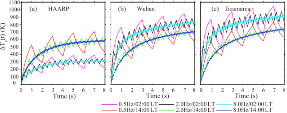
ily by investigating the electron temperature at the reflection point. A series of results of the temporal evolution of the elec-tron temperature change at the reflection point are presented in Fig. 4, and the variation of the average electron tempera-ture oscillation amplitude with different modulation frequen-cies is presented in Fig. 5. The modulation frequency sweep of 0.5, 1.0, 2.0, 4.0 and 8.0 Hz is used in the simulation.

Since in the ionospheric F2 layer the electron cooling time is tens of seconds due to the dramatically decreasing colli-sion rates and the dominating transport process (Gurevich, 1986), the electron temperature deviation from the initial background value cannot return to zero in the cooling phase of a modulation period. Moreover, the oscillation of1Tewill

finally reach a saturation state, as the results from Fig. 4 in-dicate. Also, the amplitude of the oscillation of1T_eis not a fixed value due to the drastic increase at the first modulation period. So we make an average of the amplitude of the oscil-lation of1T_ewith the value of the first period excluded, the results of which are shown in Fig. 5. When the ionospheric profile is fixed, we find that the average amplitude of the oscillation of 1Te is approximately inversely proportional

220 240 260 280 300 320 340 360 380

Height (km)

220 240 260 280 300 320 340 360 380

Height (km)

0 1 2 3 4 5 6 7

S0/Ne (10

-21_{J s}-1₎

0 1 2 3 4 5 6 7 8

Ke/Ne (10

-14_{J m}-1 _s-1 _K-1₎

0 0.5 1 1.5 2 2.5 3

(SHF+S0-Le)/Ne (10

-20_{J s}-1₎ 0 0.5 1_L 1.5 2 2.5 3

e/Ne (10

-21_{J s}-1₎

HAARP/02:00 LT HAARP/14:00 LT

Wuhan/02:00 LT

Wuhan/14:00 LT Jicamarca/02:00 LTJicamarca/14:00 LT

(a) (b)

(c) (d)

Figure 6. (a)The steady-state source termS0profile per electron; (b–d)profiles of the parallel coefficient of thermal conductivityKe, the total electron heating rateSHF+S0−Leand the electron cool-ing rate Le per electron at heating time of 1.0 s with modulation frequency of 0.5 Hz.

the ULF wave generated due to the modulated HF heating is probably undetectable on the ground. This dependence of the average amplitude of the oscillation of1Teon the

mod-ulation frequency is expected since more pump wave energy will be absorbed by the ionosphere, and the electron tempera-ture can take enough time to cool down when the modulation frequency is lower.

According to Sect. 2.1, the HF heating model is a self-consistent simulation model. Also, the background parame-ters such as plasma number density and temperature affect the electron temperature change jointly. So it is not advisable to directly relate the evolution of1T_eto a single factor from the background parameters. However, we can analyze the amplitude of the oscillation of1Tebased on the source terms

of the equations in the HF heating model. It is without doubt that the change in the electron temperature at the reflection point in a certain modulation period primarily depends on the source terms of Eq. (6). What is more, the change in elec-tron density can be negligible in a modulation period due to its much longer relaxation time than the electron tempera-ture. So the term ∂Te

∂t representing the changing rate of the

electron temperature is related to the term 2(SHF+S0−Le)

3nekB in the heating phase of a modulation period and related to the term 2Le

3nekB in the cooling phase according to Sect. 2.1. The total electron heating rate profile, SHF+S0−Le, per

elec-tron and the elecelec-tron cooling rate profile, Le, per electron

are shown in Fig. 6c and d, at the modulation frequency of 0.5 Hz. The values of the term (SHF+S0−Le)/Neat the

re-flection point in the nighttime ionosphere are 1.45_×10−20, 2.22_×10−20and 2.60_×10−20J s−1_{, which correspond to the}

HAARP case, the Wuhan case and the Jicamarca case, re-spectively. In the daytime ionosphere the corresponding val-ues are 1.70×10−20, 1.43×10−20 and 1.24×10−20J s−1. Comparing these values, we find that in the nighttime mod-ulated heating, the total heating rate per electron increases with the latitude at which the HF heating is conducted, while in the daytime it decreases with latitude. Moreover, in the midlatitudes and the equator region, the total heating rate per electron is larger in the nighttime ionosphere, while in the high-latitude region it is larger in the daytime ionosphere. The cooling rate per electron manifests the same characteris-tics as shown in Fig. 6. Since the amplitude of the oscillation of1Teis related to ∂T∂te, we can conclude thatδTemaxis

af-fected by the ionospheric profiles in the same way as the total heating rate per electron. This conclusion is obviously sup-ported by the results in Fig. 5.

3.3 Propagation and generation of ULF waves vs. modulation frequency and ionospheric parameters

In this section, we discuss the effects of modulation fre-quency and ionospheric parameters on the propagation and generation of ULF waves based on the simulation results from the model of ULF wave generation and propagation in-troduced in Sect. 2.2. In our simulation, the parameters of the electron temperature deviation Eq. (25) areδTemax=500 K, Dx₌40 km andDz₌40 km, which are fixed in all the cases of the simulation.

The magnitude of the total magnetic field vector of the ar-tificially generated ULF waves att₌2.0 s in the simulation presented in Fig. 7, in which the magnitude of the magnetic field is calculated as_|B_{| =}qB_x2₊B_y2₊B_z2. The top, middle and bottom row represent the HAARP case, Wuhan case and Jicamarca case, respectively. The left column corresponds to the generation and propagation of ULF waves in the night-time ionosphere, while the right column corresponds to the daytime case. The modulation frequency is 4.0 Hz in the sim-ulation of Fig. 7.

0 2 4 6 8 10

5 10 15 20

0

0 5 10 15

0 5 10 15 20 25

0 5 10 15

0 5 10 15 20

02:00 LT |B|(10-12_T) 14:00 LT _|B|(10-12_T)

0 200 400 600 800 1000

Height (km)

HAARP

0 200 400 600 800 1000

Height (km)

Wuhan

0 200 400 600 800 1000

Height (km)

Jicamarca

í í 0 500 1000

Horizontal distance (km)

í í 0 500 1000

Horizontal distance (km)

(a) (b)

(c) (d)

(e) (f)

Figure 7.The magnitude of total magnetic field vector of the artifi-cially generated ULF wave att=2.0 s in a simulation. The modu-lated HF heating is conducted in the ionosphere at HAARP, Wuhan and Jicamarca at 02:00 LT and 14:00 LT, and the modulation fre-quency is 4.0 Hz.

through wave propagation in the nighttime ionosphere, while in the daytime ionosphere, the wave energy is severely con-strained in the heating region, with less than 50 % of the en-ergy getting out of the region. This can be partially explained by the conclusion from Sect. 3.1. According to the definition of ULF wave wavelength in Sect. 3.1 and the Alfvén speed in Sect. 2.2, we can expect thatλ_∝n1

e when the modulation fre-quency is invariant. As depicted in Fig. 1a, the electron den-sity is larger in the daytime ionosphere, so the wavelength of ULF wave is relatively shorter. Based on the conclusion on the relation between the radiation efficiency and the wave-length in Sect. 3.1, the radiation efficiency is supposed to be lower in the daytime ionosphere than in the nighttime iono-sphere.

Now we focus on how the background parameters and the modulation frequency affect the propagation of ULF waves and their penetration to the ground. Although we can draw some conclusion from the simulation with the realistic geo-magnetic dip angles and the ionospheric profiles varying to-gether, there is no doubt that the joint effects of these two factors can make the problem more complicated and puz-zling. In order to simplify the problem without omitting the parameters we are interested in, we can focus on the HAARP case but with the dip angle assumed to be 90◦_{. The following}

discussion is based on the simulation with this assumption. Also, the modulation frequency sweep of 2.0, 4.0 and 8.0 Hz is used in this simulation.

In order to investigate the effects of the ionospheric pro-files on the propagation loss of the ULF waves, we introduce the magnetic energy of the ULF waves at a certain height within the range from −100 to 100 km in the horizontal di-rection, which is calculated as WB=R |B|

2

2µ0dx. Usually we attribute the energy loss of ULF waves in the high-latitude

0 0.5 1.0 1.5

σ_P (10- 4_{S m}-1₎

HAARP σP /02:00 LT

HAARP σP /14:00 LT

90 100 110 120 130 140 150 160 170 180 190 200

Height (km)

Figure 8.The Pederson conductivity profiles in the daytime and nighttime ionosphere at HAARP used in our simulation.

ionosphere to Joule heating because of the existence of the Pedersen current JP=σPE0 (Kelley, 2009), with σP the

Pederson conductivity and E0 the stable ionospheric

elec-tric field at high latitude. So the energy loss can be estimated byJP·δE, withδEthe electric field of the ULF waves. Both

the daytime and nighttime ionospheric Pederson conductiv-ity profiles calculated from the parameters used in the simu-lation are perceptible mainly from 200 km in the F region to the bottom of the ionosphere at 90 km, as shown in Fig. 8. So we use the magnetic energy of ULF waves at 90 and 200 km to study the propagation loss. The temporal evolution of the magnetic energy of the artificially generated ULF wave at a height of 90 km (solid line) and 200 km (dashed line) in the daytime (blue) and nighttime (red) ionosphere is presented in Fig. 9, in which the modulation frequency in this case is 2.0 Hz. The lefty axis shows the value at 200 km, while the righty axis shows the value at 90 km. We find that the magnetic energy at 200 km increases from zero and reaches a steady oscillation at the modulation frequency, while the magnetic energy at 90 km is not stable compared with that at 200 km. Since 90 km is the boundary of the ionosphere and atmosphere where the mutual conversion of ULF waves and electromagnetic waves in free space happens, this un-stable oscillation of the wave energy at 90 km is to be ex-pected. What is more important is the difference between the wave energy in the daytime and nighttime ionosphere. As depicted in Fig. 9, the magnetic energy of ULF waves at 200 km in the daytime ionosphere is much larger than in the nighttime ionosphere, while the wave energy at 90 km in the daytime ionosphere is nearly the same as in the night-time ionosphere. This feature indicates that a larger propaga-tion loss is expected in the daytime ionosphere. To present the energy loss intuitively, we make a time average of the magnetic energy at 90 and 200 km, denoting them, respec-tively, asWB90 km andWB200 km, and calculate the ratio of WB90 km/WB200 km. In this way, a smaller ratio indicates a

Ta-0 1 2 3 4 5

W

B

(10

-11

J m

-2) 200

km

0 1 2 3 4 5

W

B

(10

-14

J m

-2) 90

km

0 0.5 1 1.5 2 2.5 3 3.5 4

Time (s) Nighttime 200 km

Daytime 200 km

Nighttime 90 km Daytime 90 km

Figure 9.Temporal evolution of the magnetic energy of the artifi-cially generated ULF wave at the modulation frequency of 2.0 Hz at a height of 90 and 200 km in the daytime and nighttime ionosphere.

Table 2.Ratio between the magnetic energy of the artificial ULF wave at 90 and 200 km in the nighttime and daytime ionosphere at the modulation frequency of 2.0, 4.0 and 8.0 Hz.

Heating location Time (LT) Modulation frequency (Hz)

2.0 4.0 8.0

HAARP 02:00 0.1347 0.0755 0.0198

14:00 0.0011 0.0007 0.0004

ble 2. We find that the results support the feature that the day-time ionosphere produces more energy dissipation in wave propagation at all the modulation frequencies in the simu-lation. This can be qualitatively explained by the estimation of the energy loss due to Joule heating. According to Fig. 8, the values of the height-integrated Pederson conductivity in the daytime and nighttime ionosphere can be calculated as

P

Pday=

4.8×10−3S and P

Pnight=

2.816×10−4S, respectively, indicating a stronger Pederson current, JP. Moreover, the

wave energy at 200 km in the daytime ionosphere based on our results is much larger than in the nighttime ionosphere, which means a larger ULF electric field,δE, in most of the region where Pederson conductivity dominates. With both contributing factors larger, the daytime ionosphere is sup-posed to produce more energy loss by Joule heating. Another feature found in Table 2 is that the wave energy losses in the daytime and nighttime ionosphere both decrease when the modulation frequency increases.

Finally, we discuss the feature of the artificially excited ULF waves penetrating into the ground. The ground magni-tudes of the ULF waves at the modulation frequency of 2.0, 4.0 and 8.0 Hz in the daytime and nighttime ionosphere are demonstrated in Fig. 10. We find that both in the daytime and nighttime ionosphere, the amplitude of the magnetic field of the ULF wave decreases when the modulation frequency is enhanced from 2.0 to 8.0 Hz. According to the analysis in Sect. 3.1, the wavelength is shorter when the modulation

fre-8Hz/02:00 LT 8Hz/14:00 LT

4Hz/02:00 LT 4Hz/14:00 LT

2Hz/02:00 LT 2Hz/14:00 LT −500 −400 −300 −200 −100 0 100 200 300 400 500

Horizontal (km) 0

0.2 0.8 1.0 1.4

0.4 0.6 1.2

Ground |B| (10

-13T)

Figure 10.The ground magnitude of magnetic field of the artifi-cially generated ULF waves at the modulation of 2.0, 4.0 and 8.0 Hz in the daytime and nighttime ionosphere.

quency is raised, which makes the radiation efficiency of the ring current source lower. Moreover, the higher modulation frequency causes more propagation loss in the ionosphere as indicated in Table 2. Both factors contribute to the smaller ground magnetic field amplitude at the higher modulation frequency. When the modulation is fixed, the ground magni-tude of the ULF magnetic field is larger when the wave gen-eration and propagation happen in the nighttime ionosphere than in the daytime ionosphere. Also, this difference of the ground amplitude of the ULF wave due to the nighttime and daytime ionospheric profiles expands when the modulation increases.

4 Conclusions

Based on the HF heating model and the model of ULF wave generation and propagation, we investigate the effects of the background profiles and the modulation frequencies on the process of modulated HF heating in the ionospheric F re-gion and the subsequent generation and propagation of the artificially generated ULF waves. Some conclusions can be drawn, as follows:

2. The size of the spatial distribution ofδT_eis larger in the nighttime ionosphere than in the daytime ionosphere, and it is smaller in the ionosphere at low latitudes than at high latitudes, which indicates a higher radiation ef-ficiency of the ring current source in the daytime iono-sphere at low latitudes with a fixed ULF wavelength. 3. The background ionospheric profiles can affect the

ab-sorption of the pump wave and the cooling rate of the electron temperature during the modulated HF heating, thus determining the oscillation amplitude of δTe at a

fixed modulation frequency. The oscillation amplitude of δTe increases with latitude in the nighttime

iono-sphere, while it decreases with latitude in the daytime ionosphere. Also, the oscillation amplitude of δTe is

approximately inversely proportional to the modulation frequency.

4. The radiation efficiency of the ULF ring current source is larger in the nighttime ionosphere than in the daytime ionosphere regardless of different geomagnetic field dip angles, while the energy conversion efficiency from electron temperature oscillation to ULF waves is lower in the nighttime ionosphere with a fixedδT_einput and a fixed modulation frequency.

5. The daytime ionosphere produces more energy dissi-pation during the propagation of artificially generated ULF waves due to Joule heating, and this propagation loss is larger when the modulation frequency is raised. 6. The ground magnitude of the magnetic field of the

ar-tificial ULF wave is larger in the nighttime ionosphere than the daytime ionosphere, and the difference between daytime and nighttime conditions expands as the mod-ulation frequency increases. Also the ground ULF wave amplitude decreases when the modulation frequency in-creases.

5 Data availability

Background parameters of our numerical simula-tion used in this paper are from the Internasimula-tional Reference Ionosphere (IRI-2012) model and the neutral atmosphere model (NRLMSISE-00). These data can be accessed at the following websites: http://omniweb.gsfc.nasa.gov/vitmo/iri2012_vitmo.html and http://ccmc.gsfc.nasa.gov/modelweb/models/nrlmsise00. php.

Acknowledgements. This work was supported by the National Nat-ural Science Foundation of China (NSFC grant No. 41204111, 41574146). Chen Zhou appreciates the support by Wuhan Univer-sity “351 Talents Project”.

Topical Editor K. Hosokawa thanks three anonymous referees for their help in evaluating this paper.

References

Agrawal, D. and Moore, R. C.: Dual-beam ELF wave gener-ation as a function of power, frequency, modulgener-ation wave-form, and receiver location, J. Geophys. Res., 117, A12305, doi:10.1029/2012JA018061, 2012.

Banks, P. M. and Kocharts, G.: Aeronomy, Part A and Part B, New York, Academic Press, 1973.

Barr, R., Stubbe, P., and Kopka, H.: Long-range detection of VLF radiation produced by heating the auroral electrojet, Radio Sci., 26, 871–897, doi:10.1029/91RS00777, 1991.

Bernhardt, P. A. and Duncan, L. M.: The feedback-diffraction the-ory of ionospheric heating, J. Atmos. Sol.-Terr. Phy., 44, 1061– 1074, doi:10.1016/0021-9169(82)90018-6, 1982.

Cohen, M. B., Moore, R. C., Golkowski, M., and Lehtinen N. G.: ELF/VLF wave generation from the beating of two HF ionospheric heating sources, J. Geophys. Res., 117, A12310, doi:10.1029/2012JA018140, 2012.

Eliasson, B. and Papadopoulos, K.: Penetration of ELF currents and electromagnetic fields into the Earth’s equatorial ionosphere, J. Geophys. Res., 114, A10301, doi:10.1029/2009JA014213, 2009. Eliasson, B., Chang, C. L., and Papadopoulos, K.: Generation of ELF and ULF electromagnetic waves by modulated heating of the ionospheric F2 region, J. Geophys. Res., 117, A10320, doi:10.1029/2012JA017935, 2012.

Ferraro, A. J., Lee, H. S., Allshouse, R., Carroll, K., Lunnen, R., and Collins, T.: Characteristics of ionospheric ELF radiation generated by HF heating, J. Atmos. Terr. Phys., 46, 855–865, doi:10.1016/0021-9169(84)90025-4, 1984.

Ganguly, S.: Experimental observation of ultra-low-frequency waves generated in the ionosphere, Nature, 320, 511–513, doi:10.1038/320511b0, 1986.

Getmantsev, G. G., Zuikov, N. A., Kotik, D. S., Mironenko, N. A., Mityakov, V. O., Rapoport, Y. A., Sazanov, V. Y., Trakhtengerts, V. Y., and Eidman, V. Y.: Combination frequencies in the inter-action between high-power short-wave radiation and ionospheric plasma, J. Exp. Theor. Phys., 20, 101–102, 1974.

Greifinger, C. and Greifinger, P.: Theory of hydromagnetic propa-gation in the ionospheric waveguide, J. Geophys. Res., 73, 7473– 7490, doi:10.1029/JA073i023p07473, 1968.

Greifinger, C. and Greifinger, P.: Wave guide propagation of mi-cropulsations out of the geomagnetic meridian, J. Geophys. Res., 78, 4611–4618, doi:10.1029/JA078i022p04611, 1973.

Greifinger, P.: Ionospheric propagation of oblique hydromagnetic plane waves at micropulsation frequencies, J. Geophys. Res., 77, 2377–2391, doi:10.1029/JA077i013p02377, 1972.

Gurevich, A. V.: Nonlinear Phenomena in the Ionosphere, translated by: Liu, X. M. and Zhang, X. J., edited by: Xia, M. Y., Trans. Beijing, Science Press, 1986 (in Chinese).

Gustavsson, B., Rietveld, M. T., Ivchenko, N. V., and Kosch, M. J.: Rise and fall of electron temperatures: Ohmic heating of iono-spheric electrons from underdense HF radio wave pumping, J. Geophys. Res., 115, A12332, doi:10.1029/2010JA015873, 2010. Hansen, J. D., Morales, G. J., Duncan, L. M., and Dimonte, G.: Large-scale HF-induced ionospheric modifications: Experi-ments, J. Geophys. Res., 97, 113–122, doi:10.1029/91JA02403, 1992a.

J. Geophys. Res., 97, 17019–17032, doi:10.1029/92JA01603, 1992b.

Hughes, W.: The effect of the atmosphere and ionosphere on long period magnetospheric micropulsations, Planet. Space Sci., 22, 1157, doi:10.1016/0032-0633(74)90001-4, 1974.

Hughes, W. and Southwood, D.: The Screening of Micropulsation Signals by the Atmosphere and Ionosphere, J. Geophys. Res., 81, 3234–3240, doi:10.1029/JA081i019p03234, 1976a.

Hughes, W. and Southwood, D.: An illustration of Modification of Geomagnetic Pulsation Structure by the Ionosphere, J. Geophys. Res., 81, 3241–3247, doi:10.1029/JA081i019p03241, 1976b. Hinkel, D., Shoucri M., Smith, T., and Wagner, T.: Modeling of HF

propagation and heating in the ionosphere, Final Technical Re-port, TRW space and technology group, Griffiss Air Force Base, New York, 1992.

Istomin, Y. N. and Leyser, T. B.: Small-scale magnetic field-aligned density irregularities excited by a powerful electromag-netic wave, Phys. Plasmas, 4, 817–828, doi:10.1063/1.872175, 1997.

Kelley, M. C.: The Earth’s Ionosphere, 2nd Edn., Academic Press, Inc, San Diego, 2009.

Kotik, D. S. and Ryabov, A. V.: New results of experiment on gener-ation ULF/VLF waves with SURA facility, 2012 AGU Fall Meet-ing, Abstract ID: SA13A-2139, San Francisco, California, 2012. Kotik, D. S., Ryabov, A. V., Ermakova, E. N., Pershin, A. V., Ivanov, V. N., and Esin, V. P.: Properties of the ULF/VLF signals gen-erated by the SURA facility in the upper ionosphere, Radio-phys. Quantum El., 56, 344–354, doi:10.1007/s11141-013-9438-9, 2013.

Kotik, D. S., Ryabov, A. V., Ermakova, E. N., and Pershin, A. V.: Dependence of characteristics of SURA induced artificial ULF/VLF signals on geomagnetic activity, Earth Moon Planets, 116, 79–88, doi:10.1007/s11038-015-9465-y, 2015.

Kuo, S. P.: Ionospheric modifications in high frequency heating ex-periments, Phys. Plasmas, 22, 012901, doi:10.1063/1.4905519, 2015.

Löfås, H., Ivchenko, N., Gustavsson, B., Leyser, T. B., and Ri-etveld, M. T.: F-region electron heating by X-mode radiowaves in underdense conditions, Ann. Geophys., 27, 2585–2592, doi:10.5194/angeo-27-2585-2009, 2009.

Lysak, R. L.: Propagation of Alfven waves through the iono-sphere, Phys. Chem. Earth, 22, 757–766, doi:10.1016/S0079-1946(97)00208-5, 1997.

Lysak, R. L.: Propagation of Alfven waves through the iono-sphere:Dependence on ionospheric parameters, J. Geophys. Res., 104, 10017–10030, doi:10.1029/1999JA900024, 1999.

Lysak, R. L.: Magnetosphere-ionosphere-coupling by Alfven waves at midlatitudes, J. Geophys. Res., 109, A07201, doi:10.1029/2004JA010454, 2004.

Lysak, R. L., Waters, C. L., and Sciffer, M. D.: Modeling of the ionospheric Alfven resonator in dipolar geometry, J. Geophys. Res., 118, 1514–1528, doi:10.1002/jgra.50090, 2013.

Meltz, G., Holway, L. H., and Tomljanovich, N. M.: Ionospheric heating by powerful radio waves, Radio Sci., 9, 1049–1063, doi:10.1029/RS009i011p01049, 1974.

Moore, R. C.: ELF/VLF wave generation by modulated HF heating of the auroral electrojet, PhD thesis, Stanford University, 2007. Moore, R. C., Inan, U. S., Bell, T. F., and Kennedy, E. J.: ELF Waves

generated by modulated HF heating of the auroral electrolet and

observed at a ground distance of 4400 km, J. Geophys. Res., 112, A05309, doi:10.1029/2006JA012063, 2007.

Papadopoulos, K., Wallace, T., McCarrick, M., Milikh, G. M., and Yang, X.: On the efficiency of ELF/VLF generation using HF heating of the auroral electrojet, Plasma Phys. Rep., 29, 561– 565, doi:10.1134/1.1592554, 2003.

Papadopoulos, K., Tesfaye, B., Shroff, H., Shao, X., Milikh, G. M., Chang, C. L., Wallace, T., Inan, U., and Piddyachiy, D.: F-region magnetospheric ULF generation by modulated ionospheric heat-ing, Eos Trans. AGU, Abstract ID: SM53D-04, 88, 2007. Papadopoulos, K., Gumerov, N. A., Shao, X., Doxas, I., and Chang,

C. L.: HF-driven currents in the polar ionosphere, Geophys. Res. Lett., 38, L12103, doi:10.1029/2011GL047368, 2011a. Papadopoulos, K., Chang, C. L., Labenski, J., and Wallace, T.: First

demonstration of HF-driven ionosphere currents, Geophys. Res. Lett., 38, L20107, doi:10.1029/2011GL049263, 2011b. Park, C. G., and Banks, P. M.: Influence of thermal plasma flow

on the mid-latitude nighttime F₂layer: effects of electric fields and neutral winds inside the plasmasphere, J. Geophys. Res. 79, 4661, doi:10.1029/JA079i031p04661, 1974.

Perkins, F. W. and Valeo, E. J.: Thermal self-focusing of electro-magnetic waves in plasmas, Phys. Rev. Lett., 32, 1234–1237, doi:10.1103/PhysRevLett.32.1234, 1974.

Perkins, F. W., Oberman C., and Valeo E. J.: Parametric instabilities and ionospheric modification, J. Geophys. Res., 79, 1478–1496, doi:10.1029/JA079i010p01478, 1974.

Robinson, T. R.: The heating of the high latitude ionosphere by high power radio waves, Phys. Rep., 179, 79–209, doi:10.1016/0370-1573(89)90005-7, 1989.

Schunk, R. W. and Nagy, A. F.: Electron temperatures in the F re-gion of the ionosphere: theory and observation, Rev. Geophys. Space GE., 16, 355–399, doi:10.1029/RG016i003p00355, 1978. Schunk, R. W. and Nagy A. F.: Ionospheres of the ter-restrial planets, Rev. Geophys. Space GE, 18, 813–852, doi:10.1029/RG018i004p00813, 1980.

Schunk, R. W. and Walker, J. C. G.: Theoretical ion densi-ties in the lower ionosphere, Planet. Space Sci., 21, 1875, doi:10.1016/0032-0633(73)90118-9, 1973.

Sciffer, M. D. and Waters, C. L.: Propagation of ULF waves through the ionosphere: Analytic solutions for oblique magnetic fields, J. Geophys. Res., 107, 1297, doi:10.1029/2001JA000184, 2002. Sciffer, M. D., Waters, C. L., and Menk, F. W.: Propagation of ULF

waves through the ionosphere: Inductive effect for oblique mag-netic fields, Ann. Geophys., 22, 1155–1169, doi:10.5194/angeo-22-1155-2004, 2004.

Shoucri, M. M., Morales, G. J., and Maggs, J. E.: Ohmic heating of the polar F region by HF pulses, J. Geophys. Res., 89, 2907– 2917, doi:10.1016/0167-2789(84)90092-7, 1984.

Spitze, L.: Physics of Fully Ionized Gases, 2nd Edn., Interscience, New York, 1967.

Stubbe, P. and Kopka, H.: Modulation of the polar electrojet by powerful HF waves, J. Geophys. Res., 82, 2319–2325, doi:10.1029/JA082i016p02319, 1977.

Tepley, L. and Landshoff, R. K.: Waveguide theory for ionospheric propagation of hydromagnetic emissions, J. Geophys. Res., 71, 1499–1504, doi:10.1029/JZ071i005p01499, 1966.

Willis, J. W. and Davis, J. R.: Radio frequency heating effects on electron density in the lower E region, J. Geophys. Res., 78, 5710–5717, doi:10.1029/JA078i025p05710, 1973.

Yoshikawa, A. and Itonaga, M.: Reflection of Shear Alfvén Waves at the Ionosphere and the Divergent Hall Current, Geophys. Res. Lett., 23, 101–104, doi:10.1029/95GL03580, 1996.

Yoshikawa, A. and Itonaga, M.: The nature of reflection and mode conversion of MHD waves in the inductive iono-sphere: Multistep mode conversion between divergent and ro-tational electric fields, J. Geophys. Res., 105, 10565–10584, doi:10.1029/1999JA000159, 2000.