PRICE-SETTING POLICY DETERMINANTS:
MICRO-EVIDENCE FROM BRAZIL
*Marcelo L. Moura† José Luiz Rossi Júnior‡
Abstract
The paper studies the frequency of price changes from a survey data on Brazilian companies. The data set has the advantage of including all of the economic sectors: agricultural and food products, trading, indus-try and services. Strong evidence of nominal price rigidities is found on the data with average and median price durations around 10.1 and 8.1 months, which is very close to results reported for the euro area and the United States. Using econometric modeling through an ordered probit and also an OLS regression, we find that price change duration is mostly explained by the wage duration, the degree of competition, product spe-cialization, the elasticity of demand and economic sector dummies. The empirical results refute somewhat commonly used macroeconomic mod-eling for monetary policy evaluation; however they do not refute time-dependent models since those are consistent with different price
dura-tions across firms. These results shed light on some stylized facts that a macroeconomic price-setting model would need to reproduce.
Keywords:price-setting; frequency of price changes; nominal rigidities; sticky prices; survey data.
JEL classification:E31, D40.
1
Introduction
Price stickiness and nominal rigidities play a central role in modern
macroe-conomic models. For instance, as emphasized by Gali & Gertler(2007), the
baseline model for monetary policy evaluation relies on the assumption that
firms set prices individually on a staggered basis. Usually, a Calvo (1983)
formulation is used, where at each period there is a fixed probability that a given firm will change its price independent of its history. Although this formulation simplifies aggregation across firms and produces parsimonious aggregate supply curves, there is increasingly empirical micro evidence that price changes does not operate in this way.
The validity of those theoretical results has recently been studied empir-ically by the Inflation Persistence Network (IPN) of the European Central
*The authors would like to thank many helpful comments from an anonymous referee and Tânia
de Toledo Lima for excellent research assistance.
†Insper Instituto de Ensino e Pesquisa, email: [email protected]. ‡Insper Instituto de Ensino e Pesquisa, email: [email protected]
170 Moura and Rossi Júnior Economia Aplicada, v.14, n.2
Bank. Angeloni et al. (2006) compare recent microevidence with the main
macro models used in monetary policy analysis. Their results indicate that these models are seriously challenged by stylized facts on price-setting
prac-tices and inflation persistence. Alvarez et al. (2006) summarizes micro
ev-idence regarding price-setting policies from the analysis of panel quotes of consumer and producer prices and surveys. Their general results points to some stylized facts: i) firms change price infrequently, on average once a year; ii) price-setting behavior is heterogeneous across firms; iii) implicit or explicit contracts and coordination failure theories are important; and iv) downward price rigidity is slightly higher than upward rigidity.
The main goal of this paper is to explore the first two stylized facts
pre-sented byAlvarez et al.(2006). Our central questions are: is there evidence of
stickiness in Brazilian companies’ pricing policies? If the answer is yes, how is the frequency of price changes influenced by firms’ heterogeneity? The paper is structured as follows. Section 2 introduces a theoretical discussion con-cerning price stickiness and some of the control variables used in this study. Section 3 presents the data used in the analysis and investigates the evidence
for price stickiness. Section4studies the empirical determinants of the
dura-tions of price changes. Section 5 concludes.
2
Theoretical basis
New-Keynesian macroeconomic models usually incorporate price stickiness into the baseline model through an assumption of exogenous price changes,
as inCalvo’s1983staggered price-setting model1. InCalvo’s1983model, in
each period a fractionθof firms, 0< θ <1, reset prices, and a fraction 1−θ
of firms keep prices unchanged for at least one additional period. Assuming monopolistic competition, the problem that a particular firm faces when it has the opportunity to change its price level is to make this choice by maxi-mizing profits during the time when prices are expected to be kept fixed. The problem can be formalized as
max
p∗
t
+∞ X
k=0
θknβkhp∗tyt+k|t−C(yt+k|t) io
, (1)
subject to
yt+k|t=kp−tε, (2)
where, in equation (1),p∗tis the optimal chosen price level,βis the time
dis-count factor,yt+k|tis the expected production level int+k,given information
1Accordingly to Gali & Gertler (2007) who summarize the macroeconomic modeling
available at timetandC(·) is the firm’s cost function, which is increasing,
con-vex and twice differentiable. Equation (2) is the demand equation, wherekis
an arbitrary constant andε, is the constant elasticity of demand. In order to
have a well-defined maximization problem, we assumeε >1,.
The solution for the problem stated in (1) and (2) gives the first-order con-dition:
+∞ X
k=0
θk
(
βkyt+k|t "
pt∗−µ∂C(yt+k|t) ∂yt+k|t
#)
= 0, (3)
whereµ=ε/(ε−1) is the mark-up, a decreasing function of the demand
elastic-ity parameter,ε. Notice that, given thatε >1, the mark-up is always positive
and greater than one.
Consider the special case where firms have the opportunity to change
prices every period, this is the case of no price rigidities, withθ = 0. From
equation (3), it is easy to see that in this case the optimal price-setting will imply a constant price mark-up over the marginal cost, that is,
p∗t= ε
ε−1
∂C(yt)
∂yt . (4)
The expression in equation (4) gives an interesting benchmark case for our theoretical discussion. In the absence of rigidities, prices will change in response to changes in marginal costs or demand elasticity.
Although theoretically interesting, the equilibrium condition under flex-ible prices does not appear to be realistic. Empirical surveys indicate strong
evidence of price rigidities. Consistently with the IPN studies, like inAlvarez
et al.(2006), retail price duration in the euro area is around four to five quar-ters while in the United States is around two quarquar-ters. The same study indi-cates that the main reasons for price stickiness are the existence of implicit or explicit contracts and strategic interactions among competing firms.
Building models with endogenous price-setting rules is no simple task. Many have been developed that produce no straightforward equilibrium
con-ditions; see, for instance,Romer(1990),Kiley(2000) andBonomo & Carvalho
(2004). In general, those models allow firms to choose optimally the
proba-bility parameter of price changes, θ, implying an average price duration of
1/θ. Those models associate price changes with macroeconomic conditions;
in general, longer durations are observed with lower money growth rates and lower price variability. However, those models present no link with such mi-croeconomic conditions as demand elasticity, number of competitors or spe-cialization in one product, characteristics that our empirical study aims to investigate.
We do not intend to develop an endogenous price-setting model in this section. Instead, our goal is simply to discuss some theoretical implications of
this price-setting model2. In particular, we are interested in the shape of the
profit function with regard to the elasticity of demand. We do this by looking at the profit loss by not adjusting prices and using comparative statics to see how this profit loss depends on the elasticity of demand.
For instance, assume that at some period, there is an incentive for the
firm’s adjusting its price to the optimal level p∗, given by (4), but instead,
172 Moura and Rossi Júnior Economia Aplicada, v.14, n.2
the firm decides to keep prices fixed atp∗+∆p. Consider this profit loss
de-noted asxt≡π(p∗+∆p)−π(p∗); a Taylor second-order approximation implies
that
xt≃ ∂π
∂p p=p∗
∆p+1 2
∂2π ∂p2 p=p∗
(∆p)2
=1
2
∂2π ∂p2 p=p∗
(∆p)2
=−K(∆p)2<0,
(5)
where the second equality uses the first-order condition of profit maximiza-tion and the last one uses the second-order condimaximiza-tion for a maximum, where
K is a positive constant. From equation (4), we notice that changes in prices
are motivated only by changes in marginal costs, assuming a constant elastic-ity of demand for a given firm. Thus, substituting this into equation (5), we have
xt=−K
ε
ε−1
2
∆∂C(yt)
∂yt
!2
. (6)
Specifically, if we are interested in the effect of the elasticity of demand on
net losses
∂xt ∂ε =
2K
(ε−1)2 ε
ε−1
∆∂C(yt)
∂yt
!2
>0. (7)
This result implies that as the elasticity of demand increases, so do real net losses as a result of not adjusting prices. Assuming that there is a fixed cost in adjusting prices, the menu costs hypothesis, it is more likely that firms facing higher demand elasticity will be more inclined to change prices. Therefore, our first theoretical assumption is that firms with higher elasticity of demand will change prices more frequently, implying lower price durations. We will
test this assumption empirically in section4.
Another assumption we will test empirically concerns the relationship among the degree of concentration in the industry, measured by market share, the number of competitors, and price duration. The link we make is through the elasticity of demand. From our result in equation (4), we see that a lower elasticity implies a higher mark-up and consequently greater market power we expect will be wielded by the firm. Thus, our second theoretical assump-tion is: the higher the market power, the lower the elasticity of demand and consequently the higher the price duration.
Equation (6), shows that the profit loss depends on changes in marginal cost. However, the marginal cost also depends on the technology and the cost function. Since we have no information about the exact format of the cost function of each firm, we opt for an indirect approach to control price
adjust-ments to the cost effects. We do this by relating the profit or loss to known
effects of scale and scope. Economies of scale are defined byPanzar & Willig
(1977) when “a small pro-portional increase in the levels of all input factors can lead to more than proportional increases in the levels of outputs
(1981) is that there are economies derived from producing two or more prod-uct lines in one firm rather than producing them separately. Thus, in our final theoretical assumption, we assume that, in the presence of economies (disec-onomies) of scale and scope, the production level and the degree of product
specialization affects the frequency of price-setting. However, we make no
as-sumption with regard to whether scale and scope have a positive or negative impact on price frequency.
3
Data
We looked at a survey of 281 Brazilian firms organized by the research de-partment of Ibmec São Paulo and conducted by Sensus, a market and opinion research institute. The survey was conducted from the 3rd to the 28th of September 2007; questions were asked taking as reference the year of 2007, unless otherwise indicated. The sample was selected by using the same com-panies surveyed by Gazeta Mercantil, one of the major business newspapers in Brazil, in order to keep track of financial data of those companies and also to have a representative sample of the major business sectors of the Brazilian economy. In this way, we were able to merge data from the two independent surveys.
Table1presents the defined variables that we employed in our analysis.
Motivated by the theoretical discussion in section 2and the existent
litera-ture, we selected the wage-change duration as a proxy for cost structure; the market share or number of competitors, the level or degree of concentration
in the industry; the log of net revenues, for scale effects; the proportion of a
firm’s flagship product within total sales, for economies of scope and demand
elasticity for market conditions and mark-up effects. Notice that for
multi-product firms, the interviewer of the survey asked the interviewee to consider only the main product of the firm, the product that represents the highest per-centage of total sales. Those variables were drawn from a larger questionnaire involving a total of 90 questions. In the majority of cases, questions were an-swered at the company site by the CEO, the CFO, the director, or the financial manager.
Table2presents summary statistics for our variables of interest. Of note is
that price average and median durations for 2006/07 in Brazil are surprisingly high; the mean is 10.06 months, and the median is 12 months. Although Brazil has historically had very high inflation, particularly from 1980 to 1994, with yearly rates above 100%, we detect, for the year 2007, price durations in Brazil to be quite similar to those of the euro area and even higher than in the United States. Álvarez et al. (2006) report that for the euro area and the United States, the respective mean-price durations are 10.8 and 8.3 months. This is in accordance with the fact that CPI growth in the Brazilian economy was only 3.1% in 2006 and 4.5% in 2007, representing inflation rates just slightly above the euro area and US standards.
This result is similar to that ofGagnon(2007), who studies price-setting
174 Moura and Rossi Júnior Economia Aplicada, v.14, n.2
Table 1: Variable definitions.
Variable Survey question Answer
Price change duration ‘With what frequency does your company change prices?’
Open answer, number of months.
Wage change duration ‘With what frequency does your company change wages?’
Open answer, number of months.
Market share ‘What was the market share of your main product in 2006?’
Open answer,
Log Net revenue (R$) ‘What were the total net sales of your company in 2006?’
Open answer, thousands of Brazilian reais (R$).
Participation of the main
product ‘What is the percentage ofyour main product in total sales?’
Open answer,
Number of Competitors ‘How many competitors are in the market occupied by your main product?’
Open answer, discrete num-ber.
Demand Elasticity ‘All else being equal, in 2006, if you increase your price by 10
Source: Ibmec São Paulo / Sensus Brazilian Companies Survey
Note: Values were converted to numbers: option (a) is 0; option (b) is 2; option (c) is 4; options (d) and (e) are 8.
a much larger period than ours, encompassing a period during which infla-tion was more volatile. In fact, she finds that decreases in price durainfla-tions occurred when the economy was hit by confidence shocks, as in 2002, when
inflation hiked to 12.6%.3 Barros et al. (2009) als studies price setting in
Brazil with particular interest on the effect of variable macroeconomic
con-ditions, as market crises, change in exchange rate and monetary regimes and others. They use an unique data set from the Brazilian CPI index of Fundação Getulio Vargas with individual price-quotes from 1996-2008. Their findings also go in the same direction than the others cited above in the sense that price increases are more frequent with higher inflation, exchange rate depreciation,
higher economic activity and uncertainty.4
Regarding the other variables in table 2, we find that wage-change dura-tion is closely matched by the mean and median values for price changes; it has, however, much lower variability. With respect to competition variables, we find the market share and the number of competitors indicating the pres-ence of strong concentration in Brazilian companies; the median firm, for its main product, has around 30% of the market and 5 competitors. Mean and 3In fact, countries with a history of high inflation, like Brazil and Mexico in the 1980s and
the first half of the nineties might be associated with a lack of an anti-inflation culture. Although testing for the presence of an anti-inflation culture after price stabilization in Brazil, after 1994, would be interesting to undertake, we currently do not have the large data span necessary to test it. We thus leave this point for further research.
4We thank an anonymous referee for remembering us about the existence of a large body of
Table 2: Summary statistics
Variable Median Mean Std. Dev. Max. Min. Obs.
Price-change duration 12 10.4 8.1 60 1 195
Wage-change duration 12 11.7 2.1 24 3 255
Market share 30 35.7 32.3 100 0.000 154
Log net revenue 10.2 10 2.3 16.8 3.2 181
Revenue 26089 240174 1278565 19200000 25 181
% main product 75 68.6 30.2 100 1 109
Numb. of competitors 5 16.4 27.6 98 0 211
Demand elasticity 2 2.1 1.7 8 0.5 236
Source: Ibmec São Paulo / Sensus Brazilian Companies Survey
Net revenue in multiples of R$1,000.00 – approximately US$600.00, according to average quotes as of April 2007.
median values for the main product’s percentage of total sales indicate that Brazilian companies are generally not very diversified across products. The average demand elasticity demonstrates that the majority of Brazilian compa-nies are in the elastic region of their demand curves. The number of observa-tions across variables varies, owing to the lack of available responses to some questionnaires. Recall that, as was expressly mentioned in the questionnaire, all variables refer to the main product of each firm, which is the product re-sponsible for the most sales.
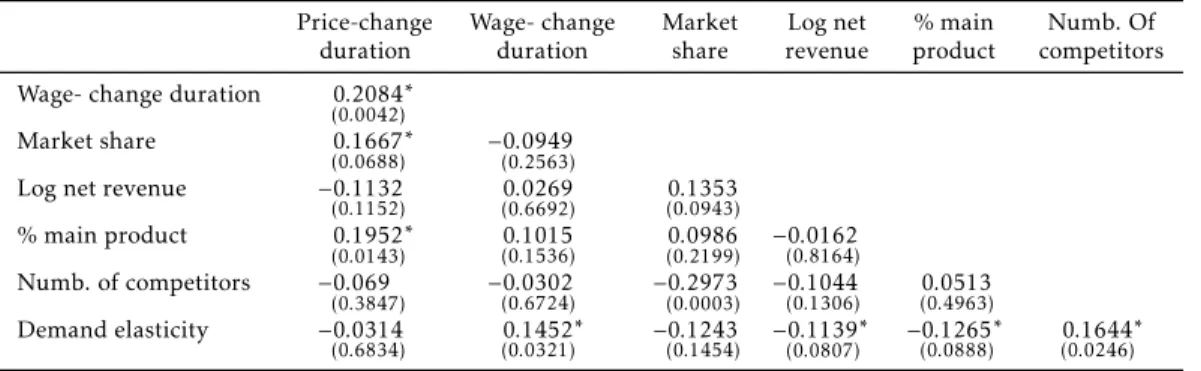
Table3presents the correlations across our variables of interest. In our
theoretical discussion in section2, we noted our expectation that price change
duration would be positively correlated to cost changes and market power. This hypothesis is partially confirmed with positive and statistically signif-icant correlations among price durations with wage-change durations and market share. Specialization (% main product) also has a positive and sig-nificant correlation with price duration, indicating possible diseconomies of scope, as price changes depend on the slope of the cost curve; see equation
. Finally, in section 2, we also mentioned that demand elasticity would be
negatively associated with market power; this is confirmed by the negative correlation of demand elasticity with market share and a positive correlation with the number of competitors.
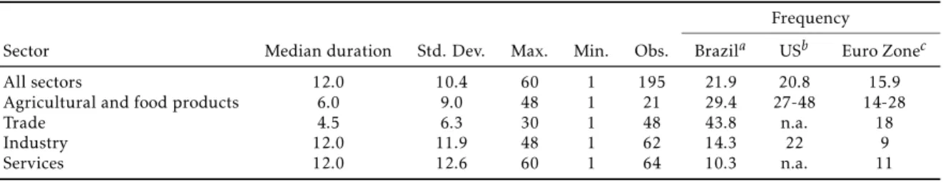
The stylized fact mentioned byAlvarez et al.(2006) regarding price
adjust-ments being heterogeneous across sectors is replicated in our survey. Table
4displays data on price frequencies across sectors and compares them with
euro-area and US data. From this, we can see a strong heterogeneity across sectors that are closely matched by euro area and US data. In general, the trading sector has longer price durations, followed by agricultural and food products. Industry and services have the longest durations and consequently lower price frequencies.
In summary, we can associate three stylized facts with our data. First, prices are indeed sticky and have high average durations. Second, data is
coherent with our theoretical hypothesis in section2. Third, price-changing
17
6
M
ou
ra
an
d
R
os
si
Jú
n
io
r
E
co
n
om
ia
A
p
lic
ad
a,
v.1
4
,
n
.2
Table 3: Correlation matrix
Price-change Wage- change Market Log net % main Numb. Of duration duration share revenue product competitors Wage- change duration 0.2084
(0.0042) ∗
Market share 0.1667
(0.0688)
∗ −0.0949
(0.2563)
Log net revenue −0.1132
(0.1152) (0.6692)0.0269 0(0.0943).1353
% main product 0.1952
(0.0143)
∗ 0.1015
(0.1536) 0(0.2199).0986 −(0.8164)0.0162
Numb. of competitors −0.069
(0.3847) −(0.6724)0.0302 −(0.0003)0.2973 −(0.1306)0.1044 (0.4963)0.0513
Demand elasticity −0.0314
(0.6834) (0.0321)0.1452
∗ −0.1243
(0.1454) −(0.0807)0.1139
∗ −0.1265 (0.0888)
∗ 0.1644
(0.0246) ∗
4
Determinants of price durations
In this section, we aim to model the firm’s decision regarding price changes as a function of market characteristics. Motivated by our theoretical discussion
in section2, we selected as potential explanatory variables the wage change
duration, as a proxy for cost structure; market share or number of competi-tors, for competition level; log of net revenues, for scale; proportion of the
main product as part of total sales, for economy of scope effects and demand
elasticity for market conditions. We also used a dummy for economic sectors in order to capture all other market specificities not captured by the previous variables.
Since our dependent variable is a discrete ordered variable, we employ an ordered qualitative response model for the price change frequency. In
par-ticular, we apply an ordered probit model, where ifyi is the price duration
choice of firmi andXi denotes the vector of firm’si characteristics, then the
probability ofyi assuming a given discrete valueJ= 0,1,2, . . . ,12, . . . ,60 is
Pr(yt=J) = Pr(y∗t< γJ) = Pr(Xiβ+ui< γJ), (8)
WhereβandγJ, J= 0,1,2, . . . ,12, . . . ,60 are the estimated parameters.
Although discrete, our dependent variable is nearly a continuous variable. Therefore, on order to test for the robustness of our results and also to make
coefficients easier to interpret, we also adopt a continuous model:
yt=α+Xiβ+ui. (9)
The regression model in (9) is estimated using ordinary least squares.
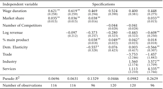
Table5reports our empirical results for the ordered probity model,
equa-tion (8), and Table6reports results for the continuous variable model,
equa-tion (9). In the two models, the results are basically the same.
The coefficient for wage-duration changes has the expected positive sign
but is not statistically significant in some specifications. As predicted in the theoretical discussion a higher competition level leads to a lower price
dura-tion; coefficients for market share are positive and significant in seven out of
eight specifications, and coefficients for the number of competitors are
nega-tive but not significant. Larger firms will also change prices more regularly,
although the coefficient is significant for just one specification in each
regres-sion model.
The level of specialization in production also seems to play an important role, as firms more devoted to one product will have higher durations and change their prices less frequently. As mentioned before, this is indicative of the presence of diseconomies of scope. The result of the demand
elastic-ity coefficient also matches the theoretical assumption that higher demand
elasticity increases real net losses by not adjusting prices and consequently
decreases price durations; see equation (7). The demand elasticity coefficient
is mostly negative and is statically significant in four out of eight cases. As
ex-pected from the analysis of section4, the industrial and service sectors have
significantly higher price duration than that shown by the other sectors, trade and agribusiness.
As a final comment, our results corroborate the empirical results of
17
8
M
ou
ra
an
d
R
os
si
Jú
n
io
r
E
co
n
om
ia
A
p
lic
ad
a,
v.1
4
,
n
.2
Table 4: Price frequency changes by sector.
Frequency
Sector Median duration Std. Dev. Max. Min. Obs. Brazila USb Euro Zonec
All sectors 12.0 10.4 60 1 195 21.9 20.8 15.9
Agricultural and food products 6.0 9.0 48 1 21 29.4 27-48 14-28
Trade 4.5 6.3 30 1 48 43.8 n.a. 18
Industry 12.0 11.9 48 1 62 14.3 22 9
Services 12.0 12.6 60 1 64 10.3 n.a. 11
aPercentage of prices that change in a given month, this value is 100/(number of months to change prices). bUnprocessed and processed food CPI data.
P
ric
e-Se
tt
in
g
P
ol
ic
y
D
et
er
m
in
an
ts
17
9
Independent variable Specifications
Wage duration 0.139
(0.054)
∗∗∗ 0.139 (0.054)
∗∗∗ 0.101 (0.061)
∗ 0.091
(0.059) (0.061)0.077 (0.064)0.115 ∗
Market share 0.006
(0.003)
∗∗∗ 0.006 (0.004)
∗∗∗ 0.007 (0.004)
∗ 0.006
(0.004)
Number of Competitors −0.006
(0.004) −(0.005)0.005
Log revenue 0.000
(0.048) −(0.061)0.084 −(0.052)0.038 −(0.054)0.085 −(0.068)0.169 ∗∗
% main product 0.010
(0.004) (0.003)0.010
∗∗∗ 0.008
(0.004)
∗∗ 0.005
(0.004)
Dem. Elasticity −0.178
(0.074) −(0.066)0.048 −(0.068)0.075 −(0.078)0.214 ∗∗∗
Trade −0.514
(0.371) −(0.451)0.563
Industry −0.712
(0.354)
∗∗ −0.871 (0.422) ∗∗
Services −0.816
(0.371)
∗∗ −1.307 (0.474) ∗∗
PseudoR2 0.028 0.028 0.0726 0.0412 0.1055 0.4651
Number of observations 116 116 0.96 120 120 96
18
0
M
ou
ra
an
d
R
os
si
Jú
n
io
r
E
co
n
om
ia
A
p
lic
ad
a,
v.1
4
,
n
.2
Table 6: OLS regression -Dependent Variables – Price-change Duration.
Independent variable Specifications
Wage duration 0.621
(0.258)
∗∗ 0.619 (0.259)
∗∗ 0.469
(0.294) (0.390)0.524 (0.381)0.400 (0.275)0.448
Market share 0.035
(0.015)
∗∗ 0.036 (0.015)
∗∗ 0.038
(0.016)
∗∗ 0.033
(0.015) ∗∗
Number of Competitors −0.044
(0.028) −(0.028)0.041
Log revenue −0.097
(0.212) −(0.257)0.373 −(0.323)0.280 −(0.322)0.443 −(0.250)0.608 ∗∗
% main product 0.038
(0.018)
∗∗ 0.049 (0.022)
∗∗ 0.042 (0.023)
∗ 0.018
(0.018)
Dem. Elasticity −0.557
(0.328)
∗ 0.076
(0.423) (0.417)0.003 −(0.307)0.566 ∗∗
Trade −3.753
(2.246) −(1.882)1.457
Industry 1.560
(2.174) (1.709)3.572 ∗∗
Services 1.113
(2.210) (1.766)4.335 ∗∗
PseudoR2 0.0696 0.0631 0.1329 0.0446 0.0982 0.2629
Number of observations 116 116 96 120 120 96
(2005) for Spanish companies, with regard to the signs and significance of competition, firm size and sector dummy variables.
5
Conclusion
The paper studied price-setting policies, using as micro-evidence survey data for 281 Brazilian companies. The analyses demonstrate interesting stylized facts, some already observed in other micro-evidence studies for the euro area and the US. The empirical results help an understanding of commonly-used macroeconomic modeling for monetary policy evaluation, particularly those models that imply nominal rigidities. New research on the topic has two equally productive veins: investment in theoretical pricing-rule models that replicate empirical stylized facts, and the further exploration of empirical
determinants of different price-setting policies across firms.
Bibliography
Alvarez, G. & Julián, L. (2008), ‘What do micro price data tell us on the
validity of the newkeynesian phillips curve?’, Economics: The Open-Access,
Open-Assessment E-Journal2(2008-19).
Alvarez, L., Dhyne, E., Hoeberichts, M., Kwapil, C., Le Bihan, H., Lünne-mann, P., Martins, F., Sabbatini, R., Stahl, H., Vermeulen, P. & Vilmunen, J. (2006), ‘Sticky prices in the euro area: A summary of new micro-evidence’,
Journal of the European Economic Association4.
Alvarez, L. & Hernando, I. (2005), Price setting behavior in spain: Stylized facts using consumerprice micro data, Working Paper Series 538, European Central Bank.
Angeloni, I., Aucremanne, L., Ehrmann, M., Galí, J., Levin, A. & Smets, F. (2006), ‘New evidence on inflation persistence and price stickiness inthe
euro area: Implications for macro modeling’, Journal of the European
Eco-nomic Association4(2-3), 562–574.
Bonomo, M. & Carvalho, C. (2004), ‘Endogenous time-dependent rules and
inflation inertia’,Journal of Money, Credit and Banking36(6), 1015–1041.
Calvo, G. (1983), ‘Staggered prices in a utility-maximizing framework’,
Jour-nal of Monrtary Economics12, 383–398.
Gagnon, G. (2007), Price setting during low and high inflation: Evidence from mexico, International Finance Discussion Papers 896, Board of Gover-nors of the Federal Reserve System.
Gali, J. & Gertler, M. (2007), ‘Macroeconomic modeling for monetary policy
evaluation’,Journal of Economic Perspectives21(4), 25–45.
Hoeberichts, M. & Stockman, A. (2004), Pricing behavior of dutch compa-nies: Main results from a survey. mimeo.
Kiley, M. T. (2000), ‘Endogenous price stickiness and business cycle
182 Moura and Rossi Júnior Economia Aplicada, v.14, n.2
Nakamura, E. & Steinsson, J. (2008), ‘Five facts about prices: A reevaluation
of menu costs models’,The Quarterly Journal of Economics123(4), 1415–1464.
Panzar, J. C. & Willig, R. D. (1977), ‘Economies of scale in multi-output
pro-duction’,The Quarterly Journal of Economics91(3), 481–493.
Panzar, J. C. & Willig, R. D. (1981), ‘Economies of scope’,The American
Eco-nomic Review71(2), pp. 268–272.
URL:http://www.jstor.org/stable/1815729
Romer, P. (1990), ‘Endogenous technological change.’, Journal of Political