*e-mail: [email protected]
Numerical Simulation of Solute Trapping Phenomena
Using Phase-Field Solidification Model for Dilute Binary Alloys
Henrique Silva Furtadoa*, Américo Tristão Bernardesb,
Romuel Figueiredo Machadob, Carlos Antônio Silvac
a
ArcelorMittal Tubarão, Av. Brigadeiro Eduardo Gomes, 930, Serra - ES, Brazil
bDepartamento de Física e REDEMAT,
Universidade Federal de Ouro Preto – UFOP,
Campus Morro do Cruzeiro, Ouro Preto - MG, Brazil
c
Departamento de Metalurgia e REDEMAT,
Universidade Federal de Ouro Preto – UFOP,
Campus Morro do Cruzeiro, Ouro Preto - MG, Brazil
Received: April 13, 2009; Revised: August 18, 2009
Numerical simulation of solute trapping during solidification, using two phase-field model for dilute binary alloys developed by Kim et al. [Phys. Rev. E, 60, 7186 (1999)] and Ramirez et al. [Phys. Rev. E, 69, 05167 (2004)] is presented here. The simulations on dilute Cu-Ni alloy are in good agreement with one dimensional analytic solution of sharp interface model. Simulation conducted under small solidification velocity using solid-liquid interface thickness (2λ) of 8 nanometers reproduced the solute (Cu) equilibrium partition coefficient. The spurious numerical solute trapping in solid phase, due to the interface thickness was negligible. A parameter used in analytical solute trapping model was determined by isothermal phase-field simulation of Ni-Cu alloy. Its application to Si-As and Si-Bi alloys reproduced results that agree reasonably well with experimental data. A comparison between the three models of solute trapping (Aziz, Sobolev and Galenko [Phys. Rev. E, 76, 031606 (2007)]) was performed. It resulted in large differences in predicting the solidification velocity for partition-less solidification, indicating the necessity for new and more acute experimental data.
Keywords: phase-field, solute trapping, dilute alloys, solidification
1. Introduction
During low velocity solidification of alloys the solid-liquid inter-face atomic diffusion is much faster then the movement of interinter-face. In that case solid-liquid equilibrium holds at interface and its com-position can be obtained by equilibrium phase diagram1.
For alloys with solute partition coefficient (ratio between solute concentration at solid side of the interface and the maximum solute concentration in the liquid phase) smaller than one and solidified under low velocities, the liquid close to the solid-liquid interface will be enriched with solute, resulting in a well known segregation phenomena, which can be detrimental to the material properties1.
Rapid solidification process (RSP) allows the solid-liquid in-terface to deviate from local equilibrium, producing solute trapping phenomena in solid phase1, which increases the solute concentra-tion in solid phase and reduces the segregaconcentra-tions in the liquid side of interface. In the limit of partition-less solidification, the solute con-centration in both phase are equal, i.e., there is no segregation. This process is useful to obtain very fine structure with uniform properties. Examples of RSP products are powders, wires and foils which can be used in powder metallurgy or in producing higher performance composite materials. As an emerging RSP technology, direct strip casting is a continuous casting process for producing as cast metallic sheet of carbon and stainless steel, aluminium, magnesium, titanium and other alloys without any further thermo-mechanical processing.
Therefore, the development of capability in predicting solute trap-ping phenomena is an important task in designing new materials and new processes.
Recently, Galenko2 developed from a mass flux balance at solid-liquid interface the following expression to predict the effect of solidification velocity on the solute partition coefficient:
k V c
V V k k c V V
V V V V
v
DS e e D
DS D
, 0
2
0 2
1 1
1
(
)
=(
−(
)
)
⋅ + −(
)
+−
(
)
(
)
+
for V < VDS (1)
and kv(V, c0) = 1 for V ≥ VDS
where V is the solidification velocity; VDS is the maximum speed for solute diffusion propagation; VD is the atomic diffusion velocity of solute at the interface (or characteristic trapping velocity) ke is the equilibrium partition coefficient and c0 is the initial solute concen-tration in the system. The velocities VDS and VD are usually obtained fitting equation 1 to data obtained experimentally.
k V k V V V V
v e D
D
( )
= ++
1 (2)
and in this dilute limit, but with VDS finite to the Sobolev’s model2, i.e:
k V
V V k V V
V V V V
v
DS e D
DS D
( )
=(
−(
)
)
⋅ + −(
)
(
)
+ 1 1 2 2 (3) Phase-field model, which is based on the concept of diffuse interface, is well known for its capability in simulating solute trap-ping phenomena2-7 and therefore can be an auxiliary tool in regard to the design of material experiments. As an example, Equation 2 using the following expression to predict VD has been demonstrated to fit perfectly the phase field simulation results on solute partition coefficient in dilute alloys3,6:VD= Dl
⋅
γ λ2 (4)
where γ ω =
(
−)
⋅( )
K k k st e e 1 1 ln (5) and Dl is the interfacial solute diffusivity (generally approximated by solute liquid diffusivity),2 λ is the solid-liquid interface thickness;ω a phase-field constant and Kst is determined through fitting Equa-tions 1 to 3 to numerical results. This model takes in consideration the dependence of VD on the equilibrium partition coefficient through the parameter defined by γ. Precisely, it states that lower values of ke can increase the characteristic velocity for solute trapping (i.e. makes it more difficult to occur). The value of Kst can be taken as a correction on γ, due to the definition of a finite solid-liquid interface thickness used in phase-field models.
The objective of the present work is to compare 2 phase field models for dilute binary alloys presented in the literature6,7 and, from their validation against analytical solution of sharp interface model, to determine the value of Kst for Ni-Cu dilute alloy and to verify its va-lidity when applied to experimental data8-10. Furthermore, the models of solute trapping described above are analyzed based on phase field results and experimental data of Si-As8,9 and Si-Bi10 dilute alloys.
2. Isothermal Phase-Field Model for
Dilute Binary Alloys
Two different dilute binary alloys phase-field models can be identified from a literature review. Those are from Kim el al.6 and from Ramires et al.7. Both were developed based on previous models for pure materials and the differences between then holds on the source term. For the present work, where the phase field variable (ϕ) ranges from +1 (solid phase) to 0 (liquid phase), the diffusion equation is as follows:
∂
∂ = −
(
− + ′ − ∇)
ϕ ξ ϕ
t M source WΦ
2 (6)
where
′ =
(
(
−)
)
Φ d
dϕ ϕ ϕ
2 1 2 (7)
and W is a model parameter which introduces the effect of interface tension in the model; ξ is another model parameter related with the interface thickness and M is a mobility term.
The source term from Kim et al.6 is as follows:
source P RT
V c c c c m S e L L e S = ′
( )
⋅( )
−(
−)
−( )
(
−)
ϕ ln 1 1
1 1 (8)
and the one from Ramires et al.7 is:
source P RT
V k c
T
m k P
m e e e = ′
( )
⋅ ⋅ −(
⋅( )
)
ϕ ln ∆ exp ln ϕ
(9) where T is the temperature; Vm is the molar volume; R is the universal gas constant; ke is the equilibrium partition coefficient; me is the liquidus slope; cSe and cLe are the equilibrium solute concentration in solid and liquid phases determined by the following equations:
c T
m L e
e
=
( )
∆ (10)c T k
m S
e e
e
=
( )
∆ (11)where ∆T = (T – Tm) and Tm is the solid-liquid equilibrium temperature of pure solvent. The terms cs and cl are de solute concentrations in solid and liquid phases, which are related to the concentration field (c) through the following relations:
c c
k P P
L e
=
⋅
( )
ϕ + −(
1( )
ϕ)
(12)c k c
k P P
s e
e
= ⋅
⋅
( )
ϕ + −(
1( )
ϕ)
(13)where P (ϕ) is a function which has the following properties:
′
( )
=( )
==
P dP
d
ϕ ϕ
ϕ ϕ 0 1; 0 (14)
P
(
ϕ =0)
=0(15)
P
(
ϕ =1)
=1(16) The P expression used in the present work is3:
P
( )
ϕ =ϕ3(
6ϕ2−15ϕ+10)
(17)The model parameter W and ξ can be determined in a similar way as for pure materials, using the following expressions6:
W=3ϖσ
λ (18)
ξ λσ
ϖ
where 2λ is the interface thickness; ω is a constant that depends on the range of ϕ that defines the interface thickness (e.g. ω = 2.2 for ϕ ranging from 0.05 to 0.95); σ is the interfacial energy.
The mobility parameter (M) can be estimated by the thin in-terface approach11. Following that Kim et al.6 and Ramires et al.7 developed different formulations. The one presented by Kim et al.6 is as follow:
1 1 2 0 2 0 M RT k
V m D W c c
e k
m e i
S e L e =
(
−)
+( )
ξ σ µξ ζ ,
(20) where Diis the interface solute diffusivity (approximated by liq-uid solute diffusivity); µ0k is the interface kinetic coefficient; and
ζ
( )
c cSe, Le is as follows:ζ ϕ ϕ ϕ c c RT V
c c P P
P c c P
S e L e m L e S e L e L e ,
( )
(
)
( )
[
( )
]
( )
[
]
( )
= ⋅ − − − − + 2 11 1 ϕϕ
ϕ ϕ ϕ
( )
( )
−(
)
∫ ⋅ − c c d S e S e 1 1 0 1 (21) The one reported by Ramires et al.7 is expressed by the equation bellow: 1 1 2 1 0 2 0 M H T A Hc D W
D m k
H c c
f
m k
f
p i T
e e f p = + ⋅ ⋅ ⋅ ⋅ ⋅ + ⋅ − ⋅
(
)
ξ σ µ ξ a ∆ ∆ ∆ (22)where ∆Hf is the heat of fusion; cp is the heat capacity at constant pressure; aT is the thermal diffusivity and A is a constant that de-pends on the form of the P(ϕ) expression and in the present work is equal to 0.231.
The isothermal solidification model is completed by a diffusion equation for the solute field. In this case the proposal of Kim et al.6 was implemented, i.e.:
∂ ∂ = ∇⋅
( )
(
)
∇ − ct D H c c
c c
S L L
L
ϕ ϕ, , ln
1 (23)
where
H
(
ϕ, ,c cS L)
= −1 P( )
ϕcL(
1−cL)
+P( )
ϕ cS(
1−cS)
(24) andD
( )
ϕ =P( )
ϕ ⋅DS+ −(
1 P( )
ϕ ⋅DL)
(25) where DS e DL are solute diffusivities in the solid and liquid phases, respectively.It is important to mention that the Kim et al.6 proposal for the solute diffusion equation has no provision for an anti-trap device as proposed by Ramires et al.7. This would be no problem as far as the interface thickness is small enough to avoid abnormal artificial solute trapping induced by the diffuse interface.
3. Numerical Implementation
Equation 6 and 23 were solved using finite volume method with uniform grid12. For the time derivative the explicit scheme was used. This one imposes a restriction in the time step due to the mesh size as following13:
∆t ∆x Dl ≤
4 (26)
however this scheme is easy to implement and has the advantage that the phase field equation does not need to be solved outside the interface thickness.
The solute trap phenomena was simulated considering a planar isotropic steady state solid-liquid interface evolution of a dilute Ni-Cu alloy (0.05 mole fraction of Cu) under different undercoolings by using a 2 dimensional (2D) model developed previously. In order to reduce processing time a domain composed by 3 nodal points in × direction (1 point inside the domain and 2 points at the borders) and 2001 nodal points in y direction was adopted. Typical processing time to reach steady state was around 30 minutes using 2 processor Xeon® 3.4 GHz with 4 GB of memory and Fortran programming language with vectorization technique. The data used in those simulations are summarized in Table 1.
4. Results and Discussion
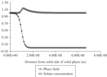
The results of present work on the solute (Cu) and phase field (ϕ) profiles along the y direction for the two dilute phase field models are presented in the Figures 1 and 2. The purpose here is to show that both results are qualitatively consistent with the physics of solidification of dilute alloys despite the differences in solidification velocities. In
Figure 1. Dimensionless steady state Cu concentration (ratio between actual concentration and solute concentration in solid at solid side of interface) and phase field profile along the y direction determined in the present work using the phase field model of Ramires et al.7: solidification velocity = 0.06 m/s
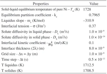
Table 1. Properties and parameters of Ni-0.05 mole fraction of Cu dilute alloy6
Properties Value
Solid-liquid equilibrium temperature of pure Ni – Tm (K) 1728
Equilibrium partition coefficient - ke 0.7965 Liquidus slope - me (K/mol) –310.9 Interfacial tension – σ (J/m2) 0.37 Solute diffusivity in liquid phase - DL (m2/s) 1.0 × 10⁻⁹ Solute diffusivity in solid phase - DS (m2/s) 1.0 × 10⁻¹⁴ Interfacial kinetic coefficient -µ
0
k (m/(sK)) 0.1
Interface thickness (2λ) (m) 8.0 × 10⁻⁹ Grid size - ∆x = ∆y (m) 1.0 × 10⁻⁹
Time step - ∆t (s) 0.5 × 10⁻¹¹
T liquidus (K) 1712.5
this case as the liquid-solid transformation evolves, the solute leaves the lower solubility solid phase to the liquid, increasing its concentra-tion close to the interface. This higher solute concentraconcentra-tion drives the diffusion process mainly in the direction of the liquid phase due to its higher diffusivity in this phase.
One of the main criticisms regarding alloy phase field models without an anti-trapping device is the artificially induced numerical solute trapping which is defined by the interface thickness used in the simulation7. This undesirable effect tends to vanish as the interface thickness tends to 0. However a very small interface thickness can lead to very large processing times. Therefore as far as the interface thickness is concerned there is a tradeoff between this undesirable numerical effect and the computational processing time.
In order to define the interface thickness to be used in the present work, simulations were performed varying the interface thickness at low solidification velocity and comparing the solute field with the one-dimensional analytical solution of sharp interface model reported by Kim et al.6 Under this condition, the phase field model should reproduce the equilibrium partition coefficient and the solute con-centration at solid side of interface should be close to the equilibrium solute concentration in this phase. Actually, as presented in Figure 3
the results using an interface thickness of 8 nanometers are in good agreement with the equilibrium condition mentioned before. In this case the numerical and analytical solutions are close to each other and the artificially induced numerical solute trapping in solid phase (solute concentration in the solid phase minus equilibrium solute concentration in this phase), was smaller than 1% of liquid bulk concentration (4.4 × 10⁻⁴ mole fraction); this error was considered reasonably small for the present study.
Another comparison of the results from the present work and an analytical solution of sharp interface model6 can be observed in the Figure 4, where the steady state solidification velocities are plotted against a range of undercoolings. Based on these results one can conclude that both models predict results with small deviation from the analytical solution.
A comparison of the effect of solidification velocity on the maxi-mum concentration close to the interface as estimated in the present work using the dilute alloy models6,7 is presented in Figure 5. It can be seen that the results are very similar. Figure 6 reports solute partition coefficient taken from models allowing for solute trapping and this work. It seems that with the appropriate values of VD and VDS the three models can fit very well the phase field results for the Ni-0.05 mole fraction of Cu alloy. Here the best fit reproduced a value of Kst equal
Figure 2. Dimensionless steady state Cu concentration (ratio between actual
concentration and solute concentration in solid at solid side of interface) and phase field profile along the y direction determined in the present work using the phase field model of Kim et al.6: solidification velocity = 0.17 m/s.
Figure 3. Solute concentration profile of Ni-0.05 mole fraction of Cu alloy along the interface, from solid side (1) to liquid side (0) at very low solidifi-cation velocity (V = 8.0 × 10⁻⁵ m/s): Model 1 means present work based on
phase field model from Kim et al.6; Analytical means one-dimensional analytic
solution of sharp interface model6.
Figure 4. Solidification velocity of Ni-0.05 mole fraction of Cu as a function of undercooling; a comparison of results from different phase field models and the analytical solution of sharp interface model: Model 1 means present work based on Kim et al.6; Model 2 means present work based on Ramires et al.7.
to 1.5. This value when used in equation 4 predicted the solute atomic diffusion velocity at interface (VD) to be 0.205 m/s.
Concerning the critical velocity to partition-less solidification (VDS) it is observed that Aziz’s model (Equation 2) approaches kv to 1 as VDS tends to infinity. Other models suggest kv= 1 for a finite VDS, which in the present Ni-Cu alloy was estimated to be 10 m/s. Nevertheless at solidification velocity of 5 m/s the results on kv for all models are around 0.99, which is very close to the partition-less solidification. It means that 1% error in the solute partition coefficient determination could change the prediction of velocity for partition-less solidification by 50%. Therefore, the precise determination of the critical velocity of partition-less solidification requires very accurate data on solute partition coefficient.
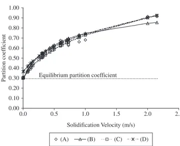
The trend of solute partition coefficient as a function of so-lidification velocity for Si-As dilute alloy is plotted in Figure 7. The experimental data are from Kittl et al.8. In this figure are also presented the best fits of equations 1 to 3. Particularly, for equation 2 the VD value was determined using equation 4 and 5 and Kst equal to 1.5. The relevant material properties used in this calculation are presented in Table 2.
As it can be seen from Figure 7 all models predicted the solute partition coefficient reasonably well up to 1 m/s. However, for higher solidification velocity Sobolev`s and Galenkos’s formula seem to better predict the partition coefficient. Nevertheless, as pointed out by Kittl et al. 8, the higher velocity experimental data have a high level of uncertainty which could lead to questionable values of VD and VDS (0.75 to 0.8 m/s and 2.1 to 2.7 m/s, respectively) reported by Sobolev`s and Galenkos’s models.
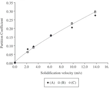
Phase-field calculation using data from Table 2, which is inde-pendent of VD and VDS, reported a trend similar to the Aziz’s model with VD predicted by equations 4 and 5 and Kst equal to 1.5 (Figure 8). Actually this trend fits the lower limit of experimental higher solidi-fication velocity partition coefficient uncertainty range. In this case, the use of Sobolev`s and Galenkos’s models to fit phase field results produced values of VD and VDS around 0.58 and 30m/s, respectively. These are very different of those obtained through fitting directly the experimental data. The reason for those large differences could be the uncertainty of experimentally obtained partition coefficient (ranging
Figure 6. The effect of solidification velocity on Cu partition coefficient: A)
Present phase-field calculations; B) best fit of equations 2,4,5; C) best fit of equation 3,4,5 using VDS = 10 m/s; and D) best fit of equations 1,4,5 using VDS=10 m/s and c0 = 0.05.
Figure 7. The effect of solidification velocity on As partition coefficient in
Si-As alloy : A) experimental8; B) equation 2 ,4 and 5 using K
st equal to 1.5;
C) Sobolev’s fitting; and D) Galenkos’s fitting.
Table 2. Data used to predict the effect of solidification velocity on solute
partition coefficient
Properties Si-As9 Si-Bi10
Equilibrium partition coefficient - ke
0.30 7.0 × 10⁻⁴ Solute diffusivity in
liquid phase - DL (m2/s)
1.8 × 10⁻⁹ 2.5 × 10⁻⁸ Solute diffusivity in
solid phase – DS (m2/s)
3.0 × 10⁻¹³ -Solid-liquid Equilibrium
tempera-ture of pure solvent (Si) - Tm (K)
1685 1685
Liquidus slope - me (K) –400
-Molar volume - Vm (m3/mol) 12 × 10-6 -Interfacial tension (J/m2) 0.472
-Figure 8. The effect of solidification velocity on As partition coefficient in
Si-As alloy: A) experimental8; B) equation 2 ,4 and 5 using K
st equal to 1.5;
from 3 to 6.5%) as well as those related to material properties used in phase-field calculation, mainly the solute diffusivities in the liquid, whose uncertain are very large (more than 30%)6,8.
Another comparison between solute trapping models is presented in Figure 9 for Si-Bi alloy. As Galenko’s and Sobolev’s models pro-duce very similar results for dilute alloys only results from Sobolev’s and Aziz’s models are presented. The experimental data are from Azis10. It can be seen that Aziz’s model with V
D determined from equations 4 and 5 and using Kst equal to 1.5 and Sobolev’s model can predict the experimental data reasonably well using VD equal to 33 m/s and VDS equal to 80 m/s.
As presented, 2 different isothermal phase field models for dilute alloy without anti-trapping device6,7 can be used to estimate the solute trapping mechanism of actual binary alloys as far as the interface thickness is small enough to avoid abnormal numerical solute trapping. From this simulation is also possible to determine a constant to be used in Azis’s formula (Equation 4 and 5) which reproduces reasonably well the effect of solidification velocity on experimentally determined solute partition coefficient in 2 different binary alloys. However, despite of the fact that one constant could be able to describe solute trapping in 2 alloys with very distinct characteristic trapping velocity, its applicability to another binary alloys must be checked using more experimental data. Furthermore, as the solute steady state concentration profile for a given interface thickness is reached, further decrease of the value of this parameter leads to a different result for Kst.
It seems from the present work that alloys with lower equilibrium partition coefficient are less prone to solute trapping, requiring a higher solidification velocity to achieve partition-less solidification. However the estimated critical velocity for partition less solidification can vary significantly depending on the solute trapping model and on the accuracy of experimental data used to determine their parameters (VD and VDS). In this case Aziz’s model will always predict a higher solidification velocity to achieve partition-less solidification (VDS) due to its asymptotic characteristic. Nevertheless, all solute trap-ping models presented here agree very well with the experimental data in the low velocity range (more accurate data) and also with the phase-field results.
Specifically for Si-As and Si-Bi dilute alloys the RSP might be a interesting process to improve conductivity of polycristaline or amor-phous semiconductor type N, due to the solute trapping effect which could extend and uniformize the solid solution of doping elements (As and Bi). Particularly for Bi this effect would be more pronounced in function of its very low equilibrium solubility in solid Si. Besides, the increase of solidification velocity beyond the partition less solidifica-tion velocity (VDS) might result in an order-disorder phase transition8, producing amorphous alloy with some peculiar properties. In this regard the solidification velocity and the consequent solid solution concentration could in principle be predicted by a simple isothermal phase-field model.
5. Conclusions
The results from two models of phase field diffusion equation6,7 reported in present work were very similar to the analytical solution of sharp interface model as far as solidification velocity and solute profile are concerned.
Using an interface thickness of 8 nanometers, the abnormal sol-ute trapping was considered very low (less than 1% of solsol-ute bulk concentration) for the present analysis.
The results of phase field solute (Cu) partition coefficient in a Ni-Cu alloy, defined as the ratio between solute concentration at the solid side of interface and the maximum concentration at the liquid phase, fitted very well to different solute trapping models of Aziz, Galenko and Sobolev.
A constant Kst equal to 1.5 determined in this fitting procedure was applied to predict the effect of solidification velocity on solute partition coefficient of Si-As and Si-Bi alloys using Aziz´s formula. The results fitted reasonably well the experimentally obtained data.
When a steady state concentration profile is reached further reduction of the interface thickness used in phase field calculations will change the value of Kst.
It seems that there is a correlation between the equilibrium parti-tion coefficient and the tendency to solute trapping. Alloys with lower solid solute solubility seem to be less prone to solute trapping.
The 3 solute trapping models and phase field results agreed rea-sonably well with the experimental data on solute partition coefficient of Si-As and Si-Bi dilute alloys, especially at the lower solidification velocity range.
The uncertainty on values of higher velocity partition coefficient in Si-As alloys leads to Galenko’s and Sobolev’s model values of VD and VDS which can be questionable.
The asymptotic characteristic of Aziz’s model will always lead to a higher solidification velocity for partition-less solidification than the other solute trapping models (Galenko e Sobolev).
It seems that for better determination of VD and VDS at higher solidification velocity, and to define the best predictive model for solute trapping, new and more accurate experimental data and mate-rial properties are required.
Concerning RSP, phase filed simulation of solute trapping phenomena could be an interesting tool to predict the solid solute concentration of doping elements (ex. As and Bi) in the Si based semiconductors, as well as the order-disorder phase transition, as far as the partition less solidification velocity can be precisely determined.
Acknowledgements
The authors are grateful to ArcelorMittal Tubarão post graduate program which partially supported this work. Funding from Brazilian agencies CNPq, CAPES and FAPEMIG is also acknowledged.
Figure 9. The effect of solidification velocity on Bi partition coefficient in Si-Bi alloy: A) experimental10; B) equation 2, 4 and 5 using K
st equal to 1.5;
References
1. Stefanescus DM. Science and Engineering of Casting Solidification. Kluwer, New York: Academic/Plenum Publisher; 2002.
2. Galenko P. Solute Trapping and diffusion-less solidification in binary system. Physical Review E 2007; 76(031606): 1-9.
3. Boettinger WJ, Warren JA, Beckermann C and Karma A. Phase-Field Simulation of Solidification. Annual Review of Materials Research. 2002; 32: 163-194.
4. Conti M. Phase and solute fields across the solid-liquid interface of a binary alloy. Physical Review E 1999; 60(2): 1913-1920.
5 Wheeler AA, Boetinger WJ and McFadden GB. Phase-Field Model of solute Trapping during solidification. Physical Review E 1993; 47(3): 1893-1909.
6. Kim SG, Kim WT and Suzuki T. Phase-field model for binary alloy. Physical Review E 1999; 60(6): 7186-7197.
7. Ramirez JC, Beckermann C, Karma A and Diepers HJ. Phase-Field Modeling of binary alloy solidification with coupled heat and solute diffusion. Physical Review E 2004; 69(051607): 1-16.
8. Kittl JÁ, Sansers PG, Aziz MJ, Brunco DP and Thompson MO. Complete Experimental Test of Kinetic Model for Rapid Alloy Solidification. Acta Materialia. 2000; 48(20): 4797-4811.
9. Danilov D and Nestler B. Phase-field modeling of solute trapping during rapid solidification of Si-As alloy. Acta Materialia 2006; 54(18): 4659-4664.
10. Aziz JM. Interface Attachment Kinetics in Alloy Solidification. Metallurgical Transaction A. 1996; 27A(3): 671-686.
11. Karma A and Rappel WJ. Phase-Field method for computationally efficient modeling of solidification with arbitrary interface kinetics. Physical Review E 1996; 53(4): R3017-R3020.
12. Patankar SV. Numerical Heat transfer and fluid flow. New York: Hemisphere Publishing Corporantion; 1980. 197 p.