Lat. Am. j. solids struct. vol.10 número3

(1)

Abs tract

In the present paper, a variationally consistent exponential shear deformation theory taking into account transverse shear deformation effect is presented for the flexural analysis of thick orthotropic plates. The inplane displacement field uses exponential function in terms of thickness coordinate to include the shear deformation effect. The transverse shear stress can be obtained directly from the constitutive relations satisfying the shear stress free surface conditions on the top and bottom surfaces of the plate, hence the theory does not require shear correction factor. Governing equations and boundary conditions of the theory are obtained using the principle of virtual work. Results obtained for static flexure of simply supported orthotropic plates are compared with those of other refined theories and elasticity solution wherever applicable. The results obtained by present theory are in excellent agreement with those of exact results and other higher order theories. Thus the efficacy of the present refined theory is established.

K ey words

exponential shear deformation theory,static flexure, orthotropic plates, shear deformation, displacements, transverse shear tresses

Flexure of thick orthotropic plates by exponential shear

deformation theory

1 INTRODUCTION

Classical plate theory [1, 2] underestimates the deflection and overestimates natural frequencies and buckling loads. This is due to not taking into account the effect of transverse shear and transverse normal stresses. The errors in deflection and stresses are quite significant for plate made out of ad-vanced composites.

First order shear deformation theory (FSDT) is considered as an improvement over the classical plate theory. Reissner [3, 4] was the first to provide consistent stress-based plate theory, which in-corporates the effect of shear deformation; whereas Mindlin [5] developed displacement based first order shear deformation theory. In these theories, the transverse shear strain distribution is as-sumed to be constant through the plate thickness and therefore, shear correction factor is required to account for the strain energy due to shear deformation. In general, these shear correction factors are problem dependent.

A . S. Say yad*

Department of Civil Engineering, SRES’S College of Engineering, Kopargaon-423601, (M.S.), India

Received 12 Dec 2011 In revised form 13 Aug 2012

*

(2)

The limitations of classical and first order shear deformation theories stimulated the develop-ment of higher order shear deformation theories, to include effect of cross sectional warping and to get the realistic variation of the transverse shear strains and stresses through the thickness of plate. For higher order theories, primarily two types of approaches are available. In one approach, the stresses are treated as primary variables. In the other approach, displacements are treated as prima-ry variables. Reddy [6] has developed well known higher order shear deformation theoprima-ry for the analysis of laminated plates considering polynomial function in-terms of thickness co-ordinate to include effect of transverse shear deformation. Many review papers are available on displacement based plate theories [7–9]. Recently many new refined theories [10-12] are developed for the analysis of isotropic and orthotropic plates. Ghugal and Sayyad [13] have developed trigonometric shear deformation theory considering effect of transverse shear and transverse normal strain/stress for the free vibration analysis of thick orthotropic plates. Shimpi and Patel [14] have developed a two vari-able refined plate theory for orthotropic plate analysis. Thai and Kim [15] applied two varivari-able plate theory for the buckling analysis of orthotropic plates using Levy type solution. Ghugal and Pawar [16] have carried out static flexure analysis of isotropic and orthotropic plates by hyperbolic shear deformation theory. Karama et al. [17] has used exponential function to predict the mechani-cal behavior multilayered laminated composite beams.

Pagano [18] has developed exact solutions within the framework of the linear theory of elasticity for rectangular bidirectional composites and sandwich plates with pinned edges. The solutions are compared to the respective solutions governed by classical laminated plate theory. However, the nature of exact solution is governed by the specific parameter which depends on the combination of the material, geometric and loading properties.

In the present work, an exponential shear deformation theory is presented for orthotropic plate analysis. The displacement model contains exponential terms in addition to classical plate theory terms. The numbers of unknown variables are same as that of first order shear deformation theory. Exact solution developed by Pagano [18] used as a basis for the comparison of results and to vali-date the present theory.

1.1 Orthotropic Plate under Consideration

Consider a plate (of length a, width b, and thickness h) made up of homogenous material. The plate occupies (in O – x – y – z right-handed Cartesian coordinate system) a region:

0≤x ≤a; 0≤y≤b; −h/ 2≤z ≤h/ 2 ₍₁₎

1.2 Assumptions made in the theory:

1. The inplane displacement u in x direction as well as displacement v in y direction each consists of two parts:

(3)

2. The transverse displacement w in z direction is assumed to be a function of x and y coordinates only.

3. The body forces are ignored in the analysis.

4. The plate can be subjected to transverse loads only.

Based upon the before mentioned assumptions, the displacement field of the present theory is given as below:

u

(

x,y,z

)

=

−

z

∂w

∂x

+

zexp −2

z h

⎛ ⎝ ⎜⎜ ⎜

⎞ ⎠ ⎟⎟ ⎟⎟

2

⎡

⎣ ⎢ ⎢ ⎢

⎤

⎦ ⎥ ⎥

⎥φ

(

x, y

)

v

(

x,y,z

)

=

−

z

∂w

∂

y

+

zexp −2

z h

⎛ ⎝ ⎜⎜ ⎜

⎞ ⎠ ⎟⎟ ⎟⎟

2

⎡

⎣ ⎢ ⎢ ⎢

⎤

⎦ ⎥ ⎥

⎥ψ

(

x, y

)

w

(

x,y,z

)

= w

(

x, y

)

(2)

Here u, v and w are the displacements in the x, y and z directions. The exponential function in terms of thickness coordinate in both the inplane displacements is associated with the transverse shear stress distribution through the thickness of plate and the functions φ and_ψ_{are the unknown} functions associated with the shear slopes. The normal strains ε

x,ε_yand shear strains γ_xy

,

γ_yz

,

γ_zx

corresponding to assumed displacement field Eqns. (2) are

ε

_x =

∂

u

∂

_x

;

ε

_y =

∂

v

∂

_y

;

γ

xy

= ∂u ∂x

+∂v ∂y

;

γ

zx

= ∂u ∂z

+∂w ∂x

;

γ

yz

= ∂v ∂z

+∂w ∂y

(3)

(4)

ε

_x =

−

z

∂

2

_w

( )

∂ψ

∂y

γ

xy =−2z

∂

2

_w

∂x

∂y+f z

=zexp −2 z

h ⎛ ⎝ ⎜⎜ ⎜ ⎞ ⎠ ⎟⎟ ⎟⎟ 2 ⎡ ⎣ ⎢ ⎢ ⎢ ⎤ ⎦ ⎥ ⎥ ⎥

The constitutive relations for orthotropic materials are as follows

σ_x =Q₁₁ε_x +Q₁₂ε_y;

σ_y =Q₁₂ε_x +Q₂₂ε_y;

τ_xy =Q₆₆γ_xy;

τ_yz =Q₄₄γ_yz;

f z

( )

∂ψ ∂y ⎡ ⎣ ⎢ ⎢ ⎤ ⎦ ⎥ ⎥;

τ_xy =Q₆₆ −2z

∂

2

_w

∂

x

∂y+f z

( )

∂φ ∂y + ∂ψ ∂x ⎛ ⎝ ⎜⎜ ⎜ ⎞ ⎠ ⎟⎟ ⎟⎟ ⎡ ⎣ ⎢ ⎢ ⎤ ⎦ ⎥ ⎥;

τ_yz =Q₄₄ df z

( )

dz ψ ⎡ ⎣ ⎢ ⎢ ⎢ ⎤ ⎦ ⎥ ⎥ ⎥

(5)

where, Q_ij are the material properties as follows:

Q₁₁₌ E1

1−_µ

12µ21

; Q₁₂ ₌ µ12E1

1−_µ

12µ21

; Q₂₂ ₌ E2

1−_µ

12µ21

;

Q₆₆ ₌G₁₂; Q₅₅ ₌G₁₃; Q₄₄ ₌G₂₃.

(7)

2 DERIVATION OF GOVERNING EQUATIONS AND BOUNDARY CONDITIONS

The governing equations and boundary conditions are derived using principle of virtual work. Let d

be the arbitrary variations

V

∫

(

δU−δW

)

∫

=0 ₍₈₎

where

δU =

0

a

∫

(

σ_xδε_x+σ_yδε_y +τ_yzδγ_yz+τ_zxδγ_zx +τ_xyδγ_xy

)

dx dy dz

0

b

∫

−h/2

h/2

∫

(9)

and

δ_W ₌

0

a

∫

q x

(

,y

)

δ_{w dx dy} 0

b

∫

(10)

Substituting Eqns. (9) and (10) in Eqn. (8)

σ_xδε_x +σ_yδε_y +τ_yzδγ_yz +τ_zxδγ_zx +τ_xyδγ_xy

(

)

0

a

∫

0

b

∫

-h /2

h /2

∫

dx dy dz

− q x,

(

y

)

0

a

∫

0

b

∫

δw dx dy =0

(11)

(6)

∂2 M_x ∂x2 +

2 ∂2

M_xy ∂_x∂_y +

∂2 M_y

∂y2 +q =

0 ₍₁₂₎

∂_N sx ∂x +

∂_N sxy ∂y

−_N

Tcx =0 (13)

∂_N sy ∂_y +

∂_N sxy

∂_x −NTcy =0 (14)

The boundary conditions are of the form:

at x = 0 and x = a

V

x =0 or w is prescribed (15)

M

x =0 or

∂w

∂x

is prescribed (16)

N

sx = 0 or φ is prescribed (17)

N_sxy ₌0 or _ψ is prescribed ₍₁₈₎

at y = 0 and y = b:

V_y = 0 _or_w_{is prescribed} ₍₁₉₎

M_y =0 or ∂w

∂y

is prescribed ₍₂₀₎

N_sxy ₌0 orφis prescribed ₍₂₁₎

N_sy ₌0 or _ψis prescribed ₍₂₂₎

M

_xy ₌0 _or_w_{is prescribed} ₍₂₃₎

(7)

M_x = σ

xz

(

)

dz

−h/2 h/2

∫

; M_y = σ

yz

(

)

dz

−h/2 h/2

∫

;

M_xy = τ

xyz

(

)

dz

−h/2 h/2

∫

; N_sx = σ

xf z

( )

⎡

⎣ ⎤⎦dz −h/2

h/2

∫

;

N_sy = σ

y f z

( )

⎡

⎣⎢ ⎤⎦⎥dz −h/2

h/2

∫

; N_sxy = τ

xyf z

( )

⎡

⎣⎢ ⎤⎦⎥dz; −h/2

∂M_xy

∂y ; Vy =

∂M_y

∂y +2

∂M_xy

∂x ⎫ ⎬ ⎪⎪ ⎪⎪ ⎪⎪ ⎪⎪ ⎪⎪ ⎪⎪ ⎪⎪ ⎪⎪ ⎪⎪ ⎪⎪ ⎪⎪ ⎪⎪ ⎪⎪ ⎪⎪ ⎭ ⎪⎪ ⎪⎪ ⎪⎪ ⎪⎪ ⎪⎪ ⎪⎪ ⎪⎪ ⎪⎪ ⎪⎪ ⎪⎪ ⎪⎪ ⎪⎪ ⎪⎪ ⎪⎪ (24)

The stress resultants in the Eqn. (24) can be expressed in-terms of functions involved in dis-placement field by Eqn. (2)

M_x =−D₁₁∂ 2_w

dx2

+Bs₁₁∂φ dx

−D₁₂∂ 2_w

dy2

+Bs₁₂∂ψ

dy (25)

M_y =−D₁₂∂

2_w

dx2 +Bs12

∂φ

dx

−D₂₂∂

2_w

dy2 +Bs22

∂ψ

dy (26)

M_xy =₋2_D 66

∂2 w

dx∂y+Bs66

∂φ dy + ∂ψ dx ⎛ ⎝ ⎜⎜ ⎜ ⎞ ⎠ ⎟⎟ ⎟⎟ (27)

N_sx =−_Bs 11

∂2_w

dx2 +Ass11 ∂_φ

dx

−_Bs 12

∂2_w

dy2 +Ass12 ∂_ψ

dy (28)

N_sy =−_Bs

12

∂2_w

dx2

+Ass₁₂∂φ dx

−_Bs

22

∂2_w

dy2

+Ass₂₂∂ψ

dy (29)

N_sxy =−2_Bs 66

∂2

w

dx∂y+Ass66

(8)

N

Tcx =Acc55φ (31)

N_Tcy ₌Acc

44ψ (32)

Using Eqns. (12) through (32) the governing equations and associated boundary conditions of the plate in-terms of functions involved in displacement field are as follows:

D₁₁

∂

4

w

w

∂

_y

4−Bs11

∂3_φ

∂x3

− _Bs

− _Ass

12+Ass66

(

)

∂

2 φ ∂_x∂_y =

0

(35)

The associated consistent boundary conditions at the edges x = 0 and x = a

−D11

∂3

w

∂x3 − D12+

4_D 66

(

)

∂

3

w

∂x∂y2+ Bs11

∂2 φ

∂x2+

2_Bs 66

∂2 φ

∂y2

⎛ ⎝ ⎜⎜ ⎜⎜ ⎞ ⎠ ⎟⎟

⎟⎟⎟+

(

Bs12+2Bs66

)

∂2 ψ

∂x∂y =

0

(36) or w is prescribed

−_D

11

∂2

w

dx2

+Bs11

∂_φ dx −_D 12 ∂2 w dy2

+Bs12

∂_ψ

dy = 0

or ∂w

∂x is prescribed (37)

−_Bs

11

∂2

w

dx2 +Ass11

∂_φ

dx −Bs12 ∂2

w

dy2 +Ass12

∂_ψ

dy =0 or φ is prescribed (38)

−2_Bs 66

∂2

w

dx∂y+Ass66

∂φ dy + ∂ψ dx ⎛ ⎝ ⎜⎜ ⎜ ⎞ ⎠ ⎟⎟

(9)

The associated consistent boundary conditions at the edges y = 0 and y = b:

−D22 ∂3

w

∂y3− D12+

4_D 66

(

)

∂

3

w

∂x2∂y− Bs22

∂2 ψ ∂y2 +

2_Bs 66

∂2 ψ ∂x2

⎛

⎝ ⎜⎜ ⎜⎜

⎞

⎠ ⎟⎟

⎟⎟⎟+

(

Bs12+2Bs66

)

∂2

φ ∂x∂y =

0 ₍₄₀₎ or w is prescribed

−D₁₂∂

2_w

dx2

+Bs₁₂∂φ dx

−D₂₂∂

2_w

dy2

+Bs₂₂∂ψ dy or

∂w

∂y

is prescribed (41)

−2_Bs 66

∂2

w

dx∂y+Ass66 ∂φ

dy +

∂ψ dx ⎛

⎝ ⎜⎜ ⎜

⎞ ⎠ ⎟⎟

⎟⎟ or φ is prescribed (42)

−_Bs 12

∂2_w

dx2

+Ass₁₂∂φ dx −Bs22

∂2_w

dy2

+Ass₂₂∂ψ

dy orψ is prescribed (43)

At corners:

−2_D 66

∂2 w

dx∂y+Bs66 ∂φ dy +

∂ψ dx ⎛

⎝ ⎜⎜ ⎜

⎞ ⎠ ⎟⎟

⎟⎟ or w is prescribed (44)

Various constants appear in governing equations and associated boundary conditions are as giv-en below:

D₁₁,D₁₂,D₂₂,D₆₆

=

(

Q₄₄,Q₅₅

)

df z

( )

dz ⎡

⎣ ⎢ ⎢ ⎢

⎤

⎦ ⎥ ⎥ ⎥ −h/2

+h/2

∫

2

dz.

⎫

⎬ ⎪⎪ ⎪⎪ ⎪⎪ ⎪⎪ ⎪⎪ ⎪⎪ ⎪⎪ ⎪⎪ ⎪⎪⎪

⎭ ⎪⎪ ⎪⎪ ⎪⎪ ⎪⎪ ⎪⎪ ⎪⎪ ⎪⎪ ⎪⎪ ⎪⎪⎪

(10)

3 NUMERICAL EXAMPLES

A simply supported rectangular plate is subjected to transverse loading

q x

(

,y

)

= q_mnsin mπx

a

⎛ ⎝ ⎜⎜ ⎜

⎞ ⎠ ⎟⎟ ⎟⎟sin n

π_y

b

⎛ ⎝ ⎜⎜ ⎜

⎞ ⎠ ⎟⎟ ⎟⎟ n=1,3...

∞

∑

m=1,3...

∞

∑

acting on the top surface (i.e., at z = – h/2), where

q

mn are the coefficients of Fourier expansion of load given as follows for various loading cases.

q mn=

16q₀

mnπ2

Uniformly distributed load

q

mn=q0 Single sine load

⎫

⎬ ⎪⎪ ⎪⎪⎪

⎭ ⎪⎪ ⎪⎪⎪

(46)

The governing differential equations and the associated boundary conditions for static flexure of plate under consideration can be obtained directly from Eqns. (12) through (23). The following are the boundary conditions of the simply supported orthotropic plates.

w

₌

_ψ

₌

M

x =Nsx

=

0

at x = 0 and x = a (47)

w

=

φ

₌

M

_y =

N

_sy

₌

0

_at_y_{= 0 and}_y₌_b ₍₄₈₎

assumed for the above exam-ples, which satisfies governing equations and boundary conditions exactly:

w x

(

,y

)

=

m=1 m=∞

∑

n=1 n=∞

∑

w_mnsinmπx

a sin

nπy

b ;

φ

(

x,y

)

=

mn, φmn and ψmn are the unknown coefficients of the respective Fourier expansions and m,

n are positive integers. In case of single sine load m = 1 and n = 1 in the above solution scheme. Substituting this form of solution and the load q x

(

,y

)

into the governing equations yields three

(11)

K11 K12 K13

K₁₂ K₂₂ K₂₃

K₁₃ K₂₃ K₃₃ ⎡ ⎣ ⎢ ⎢ ⎢ ⎢ ⎢ ⎢⎢ ⎤ ⎦ ⎥ ⎥ ⎥ ⎥ ⎥ ⎥⎥ w_mn φ_mn ψ_mn ⎧ ⎨ ⎪⎪ ⎪⎪ ⎪ ⎩ ⎪⎪ ⎪⎪ ⎪ ⎫ ⎬ ⎪⎪ ⎪⎪ ⎪ ⎭ ⎪⎪ ⎪⎪ ⎪ = q_mn 0 0 ⎧ ⎨ ⎪⎪ ⎪⎪ ⎪ ⎩ ⎪⎪ ⎪⎪ ⎪ ⎫ ⎬ ⎪⎪ ⎪⎪ ⎪ ⎭ ⎪⎪ ⎪⎪ ⎪ (50)

Eqn. (48) can be written in more concise form as follows:

K

⎡

⎣ ⎤⎦ Δ

{ }

=

{ }

q (51)

where, elements of matrix [K] and vector {Δ} are given as below:

K

11 =D11 m4_π4

a

4

+

(

2 D

12+4D66

)

m2n2_π4

a

2_b2

+ D

22 n4_π4

b4 ;

K

12 =−Bs11 m3_π3

a

3 − Bs

12+2Bs66

(

)

mn

_ab

2₂π3;

K

13 =−Bs22 n3_π3

b3 − Bs

12+2Bs66

(

)

m

_a

2n₂π3 b ;

K

22 =Ass11 m2_π2

a

2

+

Ass

66 n2_π2

b2

+

Acc

55;

K

23 =

(

Ass12+Ass66

)

mn_π2

ab

;

K

33 =Ass22 n2_π2

b

2

+

Ass66 m2_π2

a2

+

Acc

44;

Δ

{ }

= w

mn φmn ψmn

{

}

T

(52)

Unknown coefficients w

mn, φmn and ψmncan be easily evaluated using Cramer’s rule.

w_mn ₌

q_mn K₁₂ K₁₃

0 K₂₂ K₂₃

0 K₂₃ K₃₃

⎡ ⎣ ⎢ ⎢ ⎢ ⎢ ⎢ ⎢⎢ ⎤ ⎦ ⎥ ⎥ ⎥ ⎥ ⎥ ⎥⎥

K₁₁ K₁₂ K₁₃

K₁₂ K₂₂ K₂₃

K₁₃ K₂₃ K₃₃

⎡ ⎣ ⎢ ⎢ ⎢ ⎢ ⎢ ⎢⎢ ⎤ ⎦ ⎥ ⎥ ⎥ ⎥ ⎥ ⎥⎥

; φ_mn ₌

K₁₁ q_mn K₁₃

K₁₂ 0 K₂₃

K₁₃ 0 K₃₃

⎡ ⎣ ⎢ ⎢ ⎢ ⎢ ⎢ ⎢⎢ ⎤ ⎦ ⎥ ⎥ ⎥ ⎥ ⎥ ⎥⎥

K₁₁ K₁₂ K₁₃

K₁₂ K₂₂ K₂₃

K₁₃ K₂₃ K₃₃

⎡ ⎣ ⎢ ⎢ ⎢ ⎢ ⎢ ⎢⎢ ⎤ ⎦ ⎥ ⎥ ⎥ ⎥ ⎥ ⎥⎥

; ψ_mn ₌

K₁₁ K₁₂ q_mn

K₁₂ K₂₂ 0

K₁₃ K₂₃ 0

⎡ ⎣ ⎢ ⎢ ⎢ ⎢ ⎢ ⎢⎢ ⎤ ⎦ ⎥ ⎥ ⎥ ⎥ ⎥ ⎥⎥

K₁₁ K₁₂ K₁₃

K₁₂ K₂₂ K₂₃

K₁₃ K₂₃ K₃₃

(12)

Having obtained values of w x

(

,y

)

, φ

(

x,y

)

and ψ

(

x,y

)

from Eqn. (49) one can then calculate all

the displacement and stress components within the plate.

Displacements: Substituting the final solution for w(x, y), φ(x, y), and ψ(x, y) in the displacement field to obtained the inplane and transverse displacements. The expressions for these displacements are as follows:

u =

₋

z

mπ

a w

mn

+

zexp −2

z h ⎛ ⎝ ⎜⎜ ⎜ ⎞ ⎠ ⎟⎟ ⎟⎟ 2 ⎡ ⎣ ⎢ ⎢ ⎢ ⎤ ⎦ ⎥ ⎥ ⎥φmn ⎧ ⎨ ⎪ ⎪ ⎪ ⎩ ⎪ ⎪ ⎪ ⎫ ⎬ ⎪ ⎪ ⎪ ⎭ ⎪ ⎪ ⎪

cosmπx

a sin

nπy b

v =

₋

z

nπ

b w

mn

+

zexp −2

z h ⎛ ⎝ ⎜⎜ ⎜ ⎞ ⎠ ⎟⎟ ⎟⎟ 2 ⎡ ⎣ ⎢ ⎢ ⎢ ⎤ ⎦ ⎥ ⎥ ⎥ψmn ⎧ ⎨ ⎪ ⎪ ⎪ ⎩ ⎪ ⎪ ⎪ ⎫ ⎬ ⎪ ⎪ ⎪ ⎭ ⎪ ⎪ ⎪

sinmπx

a cos

nπy b

w = w

mnsin

mπx

a sin

nπy b ⎫ ⎬ ⎪ ⎪ ⎪ ⎪ ⎪ ⎪ ⎪ ⎪ ⎪ ⎪ ⎪ ⎪ ⎪ ⎭ ⎪ ⎪ ⎪ ⎪ ⎪ ⎪ ⎪ ⎪ ⎪ ⎪ ⎪ ⎪ ⎪ (54)

Inplane Stresses: The inplane normal and shear stresses (s_x,s_y, and t_xy) can be obtained by using stress-strain relations as given by the Eqns. (5) and (6).

σ_x = z Q₁₁

m

2 π2

a

2 +_Q 12 n2 π2 b2 ⎛ ⎝ ⎜⎜ ⎜⎜ ⎞ ⎠ ⎟⎟

⎟⎟⎟

w

mn

−

f z

( )

Q11

m

π

a

+Q12

nπ b ⎛ ⎝ ⎜⎜ ⎜ ⎞ ⎠ ⎟⎟ ⎟⎟φmn ⎧ ⎨ ⎪⎪ ⎩ ⎪⎪ ⎫ ⎬ ⎪⎪ ⎭ ⎪⎪sin mπx a sinnπy b

σ_y = z Q₁₂

m

2 π2

a

2 +_Q 22 n2 π2 b2 ⎛ ⎝ ⎜⎜ ⎜⎜ ⎞ ⎠ ⎟⎟

⎟⎟⎟

w

mn

−

f z

( )

Q12

m

π

a

+Q22

nπ b ⎛ ⎝ ⎜⎜ ⎜ ⎞ ⎠ ⎟⎟ ⎟⎟ψmn ⎧ ⎨ ⎪⎪ ⎩ ⎪⎪ ⎫ ⎬ ⎪⎪ ⎭ ⎪⎪sin mπx a sinnπy b

τ_xy =Q₆₆ −2_z

mn

π 2

ab

w

mn+f z

( )

nπ b φmn +

m

π

a

ψmn

⎛ ⎝ ⎜⎜ ⎜ ⎞ ⎠ ⎟⎟ ⎟⎟ ⎡ ⎣ ⎢ ⎢ ⎤ ⎦ ⎥ ⎥cos mπx a cosnπy b ⎫ ⎬ ⎪⎪ ⎪⎪ ⎪⎪ ⎪⎪ ⎪⎪ ⎪⎪ ⎭ ⎪⎪ ⎪⎪ ⎪⎪ ⎪⎪ ⎪⎪ ⎪⎪ (55)

Transverse Shear Stresses: The transverse shear stresses τ

zxandτyz can be obtained either by using the constitutive relations or by integrating equilibrium equations with respect to the thickness coordinate. The expressions for these stresses using constitutive relations are as follows:

τ_zx =Q₅₅ df z

( )

dz φmn ⎡ ⎣ ⎢ ⎢ ⎢ ⎤ ⎦ ⎥ ⎥ ⎥

cosmπx a

sinnπy b

τ_yz =Q₄₄ df z

( )

dz ψmn ⎡ ⎣ ⎢ ⎢ ⎢ ⎤ ⎦ ⎥ ⎥ ⎥

sinmπx a

cosnπy b ⎫ ⎬ ⎪⎪ ⎪⎪ ⎪⎪⎪ ⎭ ⎪⎪ ⎪⎪ ⎪⎪⎪ (56)

(13)

∂σ x ∂x

+ ∂τ

xy ∂y

+∂

τ zx ∂z

=0 (57)

∂τ

xy

∂_x +

∂σ

y

∂_y +

∂τ

yz

∂_z =0 (58)

Integrating Eqns. (57) and (58) both w.r.t the thickness coordinate z and imposing the following boundary conditions at top and bottom surfaces of the plate

τ

zx ⎡

⎣ ⎦⎤z = ± h / 2=0 ,⎣⎢⎡τyz⎤⎦⎥_{z=±h / 2}=0 (59)

Expressions for τ

zxandτyz can be obtained satisfying the requirements of zero shear stress con-ditions on the top and bottom surfaces of the plate. The following material properties are used for orthotropic plate given by Pagano [18].

E 1 E

2

=25,G12 E

2 =G13

E 2

=0.5,G23 E

2

=0.2 andµ₁₂=µ₁₃=µ₂₃=0.25 ₍₆₀₎

4 NUMERICAL RESULTS AND DISCUSSION

The displacements and stresses are obtained for different aspect ratios (S=a/h) of the plate. The results of exact elasticity theory [18] available in the literature are used as a basis for comparison of results obtained by various plate theories. The results obtained for displacements and stresses are presented in the following non-dimensional parameters.

w =w100h 3_E

2

q a4 ;

σ x, σy

(

)

=

σ x,σy qS2 ;

τ zx,τyz

(

)

=

τ zx,τyz

(

)

qS (61)

%error=

value by a particular model -value by exact elasticity solution

(14)

Table 1 Comparison of inplane displacement u_{at (}_x_{= 0,}_y₌_b_{/ 2,}_z_{= 0), deflection}w_{at (}_x₌_a_{/ 2,}_y₌_b_{/ 2,}_z_{= 0), normal}

stresses sx at (x = a / 2, y = b / 2, z = ± h / 2), normal stresses sy at (x = a / 2, y = b / 2, z = ± h / 2), and txy at (x = 0, y

= b / 2, z = ± h / 2) in orthotropic square plate subjected to sinusoidal load

S Theory Model u w σx σy τxy

4

Present ESDT 0.0094 1.5828 0.7765 0.0667 0.0312

Reddy [6] HSDT 0.0092 1.6206 0.7379 0.0640 0.0289

Mindlin [5] FSDT 0.0060 1.6616 0.4784 0.0579 0.0358

Kirchhoff [1, 2] CPT 0.0068 0.431 0.5387 0.0267 0.0213

Pagano [18] Elasticity 0.0093 1.5978 0.7276 0.0727 ---

10

Present ESDT 0.0071 0.6327 0.5809 0.0348 0.0229

Reddy [6] HSDT 0.0071 0.6371 0.5700 0.0347 0.0225

Mindlin [5] FSDT 0.0066 0.6383 0.5385 0.0339 0.0246

Kirchhoff [1, 2] CPT 0.0068 0.431 0.5387 0.0267 0.0213

100

Present ESDT 0.0068 0.4333 0.5391 0.0268 0.0213

Reddy [6] HSDT 0.0068 0.4333 0.5390 0.0268 0.0213

Mindlin [5] FSDT 0.0068 0.4333 0.5385 0.0267 0.0213

Kirchhoff [1, 2] CPT 0.0068 0.431 0.5387 0.0267 0.0213

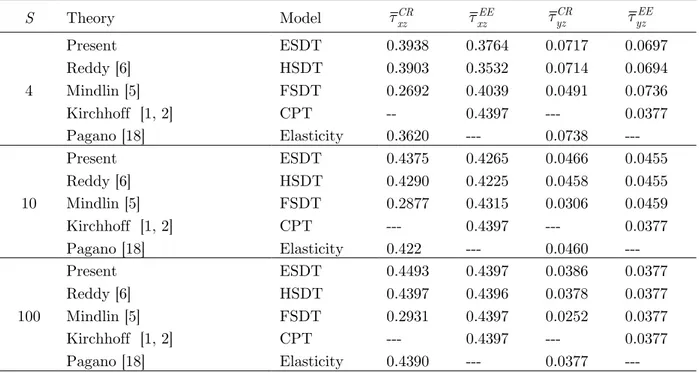
Table 2 Comparison of transverse shear stress τ

zx at (x = 0, y = b / 2, z = 0) and transverse shear stress τzy at (x = a / 2, y = 0, z = 0) in orthotropic square plate subjected to sinusoidal load

S Theory Model τ

xz CR

τ xz

EE _τ

yz

CR _τ

yz EE

4

Present ESDT 0.3938 0.3764 0.0717 0.0697

Reddy [6] HSDT 0.3903 0.3532 0.0714 0.0694

Mindlin [5] FSDT 0.2692 0.4039 0.0491 0.0736

Kirchhoff [1, 2] CPT -- 0.4397 --- 0.0377

Pagano [18] Elasticity 0.3620 --- 0.0738 ---

10

Present ESDT 0.4375 0.4265 0.0466 0.0455

Reddy [6] HSDT 0.4290 0.4225 0.0458 0.0455

Mindlin [5] FSDT 0.2877 0.4315 0.0306 0.0459

Kirchhoff [1, 2] CPT --- 0.4397 --- 0.0377

100

Present ESDT 0.4493 0.4397 0.0386 0.0377

Reddy [6] HSDT 0.4397 0.4396 0.0378 0.0377

Mindlin [5] FSDT 0.2931 0.4397 0.0252 0.0377

Kirchhoff [1, 2] CPT --- 0.4397 --- 0.0377

(15)

Table 3 Comparison of inplane displacement u at (x = 0, y = b / 2, z = 0), deflection w at (x = a / 2, y = b / 2, z = 0), normal

stresses σ

x at (x = a / 2, y = b / 2, z = ± h / 2), normal stresses σy at (x = a / 2, y = b / 2, z = ± h / 2), and τxy at (x = 0, y = b / 2, z = ± h / 2) in orthotropic square plate subjected to uniformly distributed load

S Theory Model u _w σ_x σ_y τ_xy

4

Present ESDT 0.0156 2.3368 1.0754 0.0740 0.0805

Reddy [6] HSDT 0.0147 2.3886 1.0188 0.0746 0.0739

Mindlin [5] FSDT 0.0092 2.4375 0.7041 0.0727 0.0742

Kirchhoff [1, 2] CPT 0.0104 0.6497 0.7867 0.0245 0.0464

10

Present ESDT 0.0113 0.9444 0.8341 0.0353 0.0514

Reddy [6] HSDT 0.0111 0.9506 0.8246 0.0355 0.0497

Mindlin [5] FSDT 0.0102 0.9520 0.7707 0.0353 0.0540

Kirchhoff [1, 2] CPT 0.0104 0.6497 0.7867 0.0245 0.0464

100

Present ESDT 0.0104 0.6528 0.7873 0.0246 0.0447

Reddy [6] HSDT 0.0104 0.6528 0.7871 0.0246 0.0445

Mindlin [5] FSDT 0.0104 0.6528 0.7866 0.0246 0.0465

Kirchhoff [1, 2] CPT 0.0104 0.6497 0.7867 0.0245 0.0464

Table 4 Comparison of transverse shear stress τ

zx at (x = 0, y = b / 2, z = 0) and transverse shear stress τzy at (x = a / 2, y = 0, z = 0) in orthotropic square plate subjected to uniformly distributed load

S Theory Model τ

zx CR

τ xz

EE _τ

yz

CR _τ

yz EE

4

Present ESDT 0.6542 0.6244 0.2172 0.2175

Reddy [6] HSDT 0.6567 0.6166 0.2183 0.1885

Mindlin [5] FSDT 0.4906 0.7359 0.1575 0.2362

Kirchhoff [1, 2] CPT --- 0.7806 --- 0.1846

10

Present ESDT 0.7564 0.7259 0.1935 0.1870

Reddy [6] HSDT 0.7469 0.6813 0.1909 0.1810

Mindlin [5] FSDT 0.5154 0.7731 0.1299 0.1949

Kirchhoff [1, 2] CPT --- 0.7806 --- 0.1846

100

Present ESDT 0.7970 0.7796 0.1887 0.1846

Reddy [6] HSDT 0.7800 0.7789 0.1847 0.1846

Mindlin [5] FSDT 0.5203 0.7805 0.1232 0.1847

Kirchhoff [1, 2] CPT --- 0.7806 --- 0.1846

(16)

4.1 Discussion of Results

Table 1 shows the comparison of inplane displacement, transverse (central) deflection, inplane nor-mal stresses and inplane shear stress for the orthotropic plate subjected to single sine load for the various aspect ratios. For aspect ratios (S=a/h) 10 and 100 present theory and Reddy’s [6] theory predicts exact results for inplane displacement whereas theory of Mindlin [5] and Kirchhoff [1, 2] underestimates the same. Central deflection predicted by present theory is in excellent agreement with that of exact solution for all the aspect ratios. Theories of Reddy [6] and Mindlin [5] overesti-mate the central deflection for aspect ratios 4 and 10. Present theory yields higher value for the inplane normal stress (σ

x) for all the aspect ratios whereas it is in good agreement when predicted by the theory of Reddy [6]. Inplane normal stress (σ

y) predicted by present theory is in excellent

agreement with exact solution. Reddy [6] underestimates the value of inplane normal stress (σ y) for all the aspect ratios. CPT [1, 2] and FSDT [5] yield the lower values for inplane normal stresses for all the aspect ratios.

Comparison of transverse shear stresses for the orthotropic plate subjected to single sine load is presented in Table 2. Examination of Table 2 reveals that, for S = 4, present theory overpredicts the value of maximum transverse shear stress (τ

zx) by 8.781 % when obtained using constitutive relation (τ

xz CR

) and overpredicts the same by 3.98 % when obtained using equilibrium equations (τ

xz

EE_{). For}

S=10, present theory and theory of Reddy [6] shows good accuracy of results. CPT [1, 2] and FSDT [5] overestimate the value of maximum transverse shear stress (τ

xz

EE_{) when obtained}

via equations of equilibrium. Present theory and theory of Reddy [6] shows good accuracy of results for maximum transverse shear stress (τ

yz) when obtained using constitutive relation.

Comparison of deflection and stresses of an orthotropic plate subjected to uniformly distributed load are shown in Tables 3 and 4. Observation of Table 3 shows that, present theory predicts higher value of inplane displacement for all the aspect ratios. The central deflections predicted by the pre-sent theory are in close agreement with those of exact elasticity solution for all the aspect ratios. The percentage error in central deflection is -0.94 %, -0.27 % and 0.015 % using present theory for aspect ratios 4, 10 and 100 respectively. The Reddy’s theory [6] and Mindlin’s theory [5] overpre-dicts the value of central deflection. The present theory yields the improved inplane normal stresses compared to other theories. The percentage error in inplane normal stress (σ

(17)

5 CONCLUSIONS

In this paper, exponential shear deformation theory is applied to static flexure of square orthotropic plates and following conclusions are drawn from the study.

1. It is variationally consistent displacement based refined shear deformation theory.

2. The constitutive relations are satisfied in respect of inplane stress and transverse shear stress. 3. The transverse shear stresses satisfy shear stress free boundary conditions at the top and bot-tom faces of the plate hence the theory does not require shear correction factor.

4. It is observed that the results of central deflection predicted by proposed theory is in excellent agreement with the exact results.

5. Inplane stresses predicted by proposed theory are in good agreement with the exact results and other higher order theories.

6. The proposed theory is capable of producing reasonably good transverse shear stresses using constitutive relations, and better values of these stresses can be obtained by integration of equilibri-um equations.

References

[1] G.R. Kirchhoff. Uber das gleichgewicht und die bewegung einer elastischen scheibe. Journal of Reine Angew. Math. (Crelle), 40:51-88, 1850.

[2] G.R. Kirchhoff. Uber die uchwingungen einer kriesformigen elastischen scheibe, Poggendorffs Annalen. 81:58-264, 1850.

[3] E. Reissner. On the theory of bending of elastic plates. Journal of Mathematics and Physics, 23:184-191, 1944. [4] E. Reissner. The effect of transverse shear deformation on the bending of elastic plates. ASME Journal of

Ap-plied Mechanics, 12:69-77, 1945.

[5] R.D. Mindlin. Influence of rotatory inertia and shear on flexural motions of isotropic, elastic plates. ASME Journal of Applied Mechanics, 18:31-38, 1951.

[6] J. N. Reddy. A simple higher order theory for laminated composite plates. ASME Journal of Applied Mechan-ics, 51:745-752, 1984.

[7] Y.M. Ghugal and R.P. Shimpi. A review of refined shear deformation theories for isotropic and anisotropic laminated plates. Journal of Reinforced Plastics and Composites, 21: 775-813, 2002.

[8] W. Chen and W. Zhen. A selective review on recent development of displacement-based laminated plate theo-ries. Recent Patents on Mechanical Engineering, 1:29-44, 2008.

[9] I. Kreja. A literature review on computational models for laminated composite and sandwich panels. Central European Journal of Engineering, 1(1):59-80, 2011.

[10] R. P. Shimpi. Refined plate theory and its variants. AIAA Journal, 40(1): 137-146, 2002.

[11] R. P. Shimpi, H. G. Patel and H. Arya. New first order shear deformation plate theories. Journal of Applied Mechanics, 74: 523-533, 2007.

[12] Y. M. Ghugal and A. S. Sayyad. A flexure of thick isotropic plate using trigonometric shear deformation theo-ry. Journal of Solid Mechanics,2(1):79-90, 2010.

[13] Y. M. Ghugal and A. S. Sayyad. Free vibration analysis of thick orthotropic plates using trigonometric shear deformation theory. Latin American Journal of Solids and Structures, 8: 229-243, 2011.

[14] R. P. Shimpi and H. G. Patel. A two variable refined plate theory for orthotropic plate analysis. International Journal of Solids and Structures, 43:6783-6799, 2006.

(18)

[16] Y. M. Ghugal and M. D. Pawar. Flexural analysis of thick plates by hyperbolic shear deformation theory. Journal of Experimental & Applied Mechanics, 2(1):1-21, 2011.

[17] M. Karama, K. S. Afaq and S. Mistou. Mechanical behavior of laminated composite beam by new multi-layered laminated composite structures model with transverse shear stress continuity. International Journal of Solids and Structures, 40:1525–1546, 2003.