(Recebido em 05/11/2008; Texto Final em 14/08/2009).
(Estudo Preliminar do Comportamento Mecânico de Soldas a Ponto por Fricção)
José Antônio Esmerio Mazzaferro1,2, Tonilson de Souza Rosendo1,2, Cíntia Cristiane Petry Mazzaferro1,2, Fabiano Dornelles Ramos2,3, Marco Antônio Durlo Tier2,3, Telmo Roberto Strohaecker1, Jorge Fernandes dos Santos2.
1Universidade Federal do Rio Grande do Sul/PROMEC-DEMEC, Porto Alegre, Rio Grande do Sul, Brazil
2GKSS Research Centre/Institute of Materials Research-Materials Mechanics Solid State Joining Processes (WMP), Geesthacht, Germany
3Universidade das Missões/Departamento de Engenharia e Ciências de Computação, Santo Ângelo, Brazil [email protected]
Abstract
The Friction Spot Welding - FSpW is a solid-state process that allows joining two or more metal sheets in lap configuration with no residual keyhole as occurs in the Friction Stir Welding - FSW process. The present work reports part of the efforts made at GKSS Research Centre to better understand the complex phenomena that take place during FSpW of aluminum alloys and establish the mechanical response of the resulting joints. Over the recent years the research on modeling friction based welding processes has increased considerably. Most of the works related to this subject deal with the process mechanics. On the other hand, some investigations have shown how the process variables affect the mechanical properties of the joints, but it is very difficult to find quantitative results that can be readily used for mechanical design purposes. The aim of this work is to develop an analysis procedure based on the process characteristics that allows evaluating how the resulting geometry and microstructure affect the joint mechanical behavior. For this, the results of the mechanical tests obtained on AA2024-T3 aluminum alloy were used to calibrate and validate a numerical model that was used to predict the joint failure mode. The model reproduced the specimen geometry and load conditions adopted in the lap-shear and cross-tensile tests. The joint was considered as formed by three main regions (SZ – stir zone, TMAZ – thermo mechanically affected zone and HAZ – heat affected zone) whose properties and dimensions were based in microhardness evaluation and macrographic analysis of welded specimens. It was observed a good agreement between the simulation results and experimental data. The numerical modeling of the joints allows the prediction of the joint mechanical properties, as well as to understand how a change in geometry and property of each region affects the final mechanical behavior. Based in the obtained results, the analysis procedure can be easily extended to the related friction based spot processes as Friction Stir Spot Welding – FSSW.
Key-words: Friction Spot Welding, FSpW, failure mode
Palavras Chave:Soldagem por fricção a ponto, modo de falha
Introduction 1.
The research associated to friction based process has considerably increased in the last years. This fact can be explained by the various advantages of these processes when compared to the conventional fusion welding process. The advantages become more evident in situations where the conventional processsimplycannotbeused,asincaseofdificultweldability orwhenjoiningdissimilarmaterials.
Thefocusoftheworkwasconcentratedinthedevelopment of a computer model to simulate the welding joint behavior under typical loading conditions.
Currently, the analysis had been concentrated on the Friction Spot Welding (FSpW), a spot welding process invented and patented by GKSS. This process can represent an alternative to conventional spot welding processes like Resistance Spot Welding (RSW) and Riveting if could be demonstrated that the mechanical behavior of the resulting joints is similar. In this way, the numerical simulation can be an attractive and eficient instrument to decrease the number of actual welding tests, shortening the technology development time in this area. Even,thepossibilityoftestvirtuallytheeffectofdifferentweld conditions/parameters over the resulting mechanical behavior and predict the failure mode under typical load conditions, can make simulation an useful instrument in estimation of potential service performance of mechanical elements containing FSpW joints.
Although some experience from previous studies has been obtained in dealing with the related process FSW, the Friction based Spot Welding Processes present their particular characteristics and joint mechanical behavior.
SincetheFSWprocesswasprimarilydevelopedandknown asapotentiallynewimportantweldingjoiningmethod,numerous studies have been conducted to allow a better understanding of its fundamentals. The irst efforts to model analytically and numerically the FSW process had been conducted by Bendzsak et al in 1997 [11]. Others, such as Chao and Qi in 1999 [2] Colegrove in 2000 [3], Ulysse in 2002 [5], Xu et al [4] and Arbegast [6] in 2003, and Schmidt et all in 2004 [7] can be cited as signiicant contributors to the best understanding of the processphysics,orproposednewmethodstosolvethehighly non linear problem. These efforts are extended to FSSW and FSpW [8, 9, 10] and the modeling methodologies are thought to become stronger instruments for future tool design, process optimization and control of these process.
Speciically in the friction based welding processes, these tools have been used to predict temperature, stress ields and material low around the tool. The numerical and analytical models available in the literature present different approaches, assumptionsandlevelsofcomplexity.Inthepresentworkthe objective is not to simulate the FSpW process itself but produce amodelthatallowsdeterminingtheresultingjointmechanical response.
Model Development 2.
The numerical model was developed considering the speciicities of the Friction Spot Welding process, the equipment used to produce the bonding region and the mechanical tests available for model validation.
FSpW characteristics 1.1
To correctly model the contact region between the welded plates, some characteristics of the welding equipment can be taken in consideration.
AsseeninFigure1theweldingmachineconsistsbasicallyof amainhead,wheretoolsofdifferentgeometriescanbeadjusted. Therotatingtool,whichcanbealsoseenintherighthandside of the igure, exhibits no traverse movement, what means the joint geometry is symmetric in both longitudinal and transversal directions.Inthisway,thestirzoneshapewilldependonlyof tool geometry and the variant of the process chosen.
Figure1.PrototypemachineforFSpWandweldingtool[12].
The FSpW tool is formed by an external clamping ring, a shoulder, and an internal pin. The model used in simulation wasdevelopedconsideringthedimensionsofthetoolusedto produce the FSpW joints: the pin and shoulder diameters are respectively 5.2 mm and 9.0 mm [12].
Regardingtheprocessvariant,therearebasicallytwoways the tool can penetrate in the plates, called the pin plunge and the shoulder plunge variants of the process.
Oncethecontactisestablished,thesequenceofstepsshown on the left and right hand sides describes the pin plunge and shoulder plunge variants respectively.
As can be seen, in the irst step of the pin plunge variant the shoulderretractswhilethepinpenetratesintheplatessqueezing the plasticized base metal to ill up the cavity formed by the shoulder movement. In the shoulder plunge variant the relative movementbetweenpinandshoulderoccursinoppositeways.
In the second stage pin and shoulder return to their initial position, corresponding to the top of the upper plate before the start of plunge step.
Finally,thetoolretractswithnorelativemovementbetween its parts. The cross section of the resulting weld spots will be determined by this sequence of events. There are speciic characteristics associated to each one of these variants, but whatdeinesthejointstrengthistheshapeoftheresultingspot
weld.Alltheexperimentalresultspresentedinthisworkwere obtained using the shoulder plunge variant, which produces a greatereffectiveplates’contactareaafterwelding.
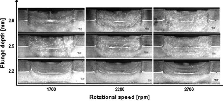
Figure 3 presents some macrographic images of AA2024-T3 FSpW joints to different plunge depths and rotational speeds.
Wecanobservethat,regardingthevariationofthewelding parameters, the stir zone width did not show evidence of change.Hence,themodelgeometrydeinitionwasbasedontool dimensions and plates coniguration actually used in mechanical tests.
Analyzing the macrographs, it is possible to observe the formationofregionswithdiversegrainsizesandorientations. TheseregionsaredesignedStirZone–SZ,Thermo-Mechanically AffectedZone–TMAZ,HeatAffectedZone–HAZandBase Metal–BM.Adetaileddescriptionoftheircharacteristicscan be found in [13].
Figure 3. Macrographic images of different shoulder plunge FSpW joints of AA2024-T3 [12, 14].
In the macrographs is possible to easily identify the approximate boundary between SZ, TMAZ and BM, as seen in Figure 4. It is possible to verify that, depending on process parameters, the clad layer can be more or less dispersed in SZ. Thiswasnotconsideredinthenumericalmodel.Inthedetailof Fig. 4 it is possible to see that there is a great difference in grain sizebetweenSZandTMAZ,whilegrainsofTMAZandHAZ are similar.
Based in this general aspect of a typical joint produced by the toolusedtoperformtheactualwelds,themodeljointgeometry wasdeinedasshowninthesketchofFigure5.
Figure5.Geometryofthedifferentweldingzonesdeinition for modeling purposes.
The sketch shows the interface between the two welded platesinlapconiguration,aswellasthedifferentjointregions. Thedashedbluelinerepresentsthecentreoftheweld,where theSZcanbeseenexactlywherethetoolpenetratessqueezing and plasticizing the base metal. Around the periphery of SZ is located the TMAZ, where a constant width of 0.75 mm was assumed, and beyond its external boundary, the BM that did not has experienced any microstructure change. The dimensions assumedfortheregionsweredeinedconsideringthesimplicity to model using simple features like lines and curves, and that the critical points should coincide with plate boundaries to avoid errors in contact between the just created surfaces and mesh geometry. The values are function of tool geometry and processing parameters, not changing appreciably to the range of parameters studied. It is worth noting that no HAZ was consideredinthemodel,whatcanbeexplainedbythesimilar mechanical properties of these adjacent regions.
Material Properties 1.2
The base material used in the simulations was theAlclad AA2024-T3 2 mm thick plate. This choice was based on its massive use in aircraft industry and the large number of experimentaldataavailablefrompreviousworks[12,14,15,16, 17].ThechemicalcompositionofthealloyisshowninTable1. The main mechanical properties of the alloy in T3 condition are: yield strength e = 310 MPa, ultimate tensile strength r = 448 MPa, elongation = 20 %.
Table 1. Chemical composition of the AA2024.
Grade Si Fe Cu Mn Mg Zn Ti Al
2024 0.19 0.23 3.94 0.55 1.24 0.22 0.02 bal.
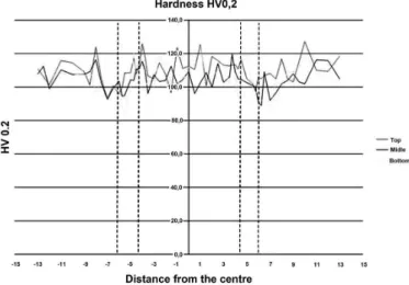
OncetheBMwaschosen,thepropertiesoftheotherweld regions should be deined. Since no mechanical test data on the propertiesofeachregionwereavailable,thehardnessproiles of an actual welded specimen were used to estimate these properties.
ThegraphshowninFigure6presentsthehardnessproile along the cross section of the joint at three different distances from the upper plate top surface. The vertical dashed lines deine the approximate position of SZ and TMAZ boundaries.
Analyzingthehardnessproileitisobservedthattherewas nosigniicantchangeinhardnessbetweenthedifferentregions. We can see a slightly hardness decrease in the boundary region betweenTMAZandBM.
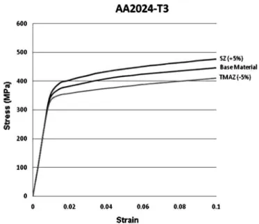
Based on the hardness proile, three different property settingswereassumed(Figure7).
The middle line shows the engineering stress-strain curve correspondingtothebasemetalproperties.Itwasassumedthat in the SZ region the mechanical resistance is 5% greater than that in the base metal, as indicates the upper line. On the other hand, in the TMAZ, a decrease of 5% from base metal resistance wasconsidered,asshowninthelowercurvebehavior.Asstated
before,thesevalueswerebasedinthehardnessobservedineach joint region.
Figure 7. Engineering stress-strain curves assumed for BM, SZ and TMAZ.
Model Characteristics 1.3
The solid model was developed using the commercial packages SolidWorks – CAD andAbaqus – CAE [11]. Once the3DsolidpartsweremodeledinSolidWorks,thegeometry was exported to Abaqus, where the assembly of components and speciication of contact and boundary conditions, loads, and meshcharacteristicswerecarriedout.
Each one of the modeled welding joints was composed of threedifferentparts:theStirZone,anUpperPlateandaLower Plate, as seen in Figure 8.
Figure 8. Welded joint composed of three different 3D parts.
TheSZ,whosedimensionswereshownpreviouslyinFigure 5, and properties correspond to a mechanical resistance 5% higher than in BM.
TheupperplatecontainsaholewheretheSZisaccommodated and a region of constant distance around this hole that represents the TMAZ. In this region, nearby the hole, the properties correspondtotheTMAZ,whileintherestoftheplatetheBM
propertieswereused.
Thelowerplateexhibitsafeaturecorrespondingtoholeleft when removing SZ.As occurs in the upper plate, a region of constant width around this feature represents theTMAZ.The rest of the plate corresponds to base metal.
The assembly of the model consists of place each part in its correct relative position as can be seen in the Figure 9.
Figure 9. Aspect of the joint after assembly.
Modeling the problem as described, makes easy to assign different properties to each region, control the mesh creation and establishthecontactbetweeneachoneoftheparts.
Oncedeinedtheweldzonesdimensionsandtheproperties of each region, the full model geometry deinition was based on plates’ coniguration, loading and boundary conditions actually used in mechanical test specimens. The specimens currently modeled correspond to lap-shear and cross-tensile test specimens.
Lap-Shear Specimen
The DIN EN ISO 14272 standard deines conditions for lap-shear and cross-tensile tests. As shown schematically in Figure 10-a, two plates welded by FSpW in lap coniguration are submitted to a uniaxial tensile load. To avoid misalignment of the plates and out of plane loading during the test, shims (represented in orange color in the igure) are placed bellow each plate.
Figure 10. Schematic specimen representation from DIN EN ISO 14272: a) lap-shear and
b) cross-tensile specimen, adapted from [13].
specimen size is very important to minimize the total number of inite elements necessary to represent it. Consequently the required computational resources and cost associated to the numerical simulation are reduced.
Figure 11. Lap-shear model geometry and boundary conditions.
As shown in the igure the extremity of the lower plate was pinned, what means that the displacements in the three orthogonaldirections(x,yandz)weresetequaltozero.Also, theverticalmovementoftheexternalportionofbothplateswas not allowed, to reproduce the effect of test machine clamps. To simulate the actual load condition experimented during the test,adisplacementoftheexternalsurfaceofupperplatewas speciied.
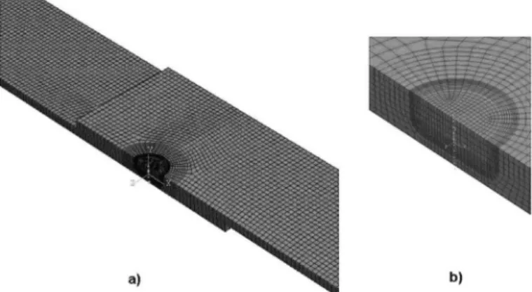
Ahexahedralstructuredmeshwascreatedinalltheregions of each one of the three parts where eight node linear brick elements were used. The reduced integration was adopted to avoidthevolumetriclockthatcanhappenwhen3Dsolidmodels are used [11]. The Figure 12-a presents the general aspect of the resultingmeshandinFigure12-badetailoftheweldregionis shown.
Figure12.Aspectofthemeshcreated:a)generalviewandb) detail of the region of interest.
As the highest stresses are developed in the region of contact betweentheplates,themeshdensityshouldbegreaterinthis area. Also it is possible to notice in the detail the coherency betweenadjacentelementsinthedifferentparts.Inthismodel thetotalnumberofelementswasabout28000.
Cross-Tensile Specimen
The cross-tensile specimen was shown schematically in Figure10-b.Usingaspeciicdevice(notshownintheigure)
twoplatesweldedbyFSpWinlapconigurationaresubmitted toaverticaltensileloadthatseparatesthem.Thedeviceallows the vertical movement of the central overlapped portion of both plates,whilekeepstheexternalportionofeachpartrestricted.
Figure 13 presents the geometry, boundary conditions and loading used in the cross-tensile model. In this case, the entire specimen had to be modeled to avoid unrealistic results.
Figure 13. Cross-tensile model geometry and boundary conditions.
To reproduce the test the following boundary conditions wereusedinthemodel:theexternalportionsoflowerplatehad its vertical movement constrained while a displacement was speciiedtotheexternalportionsoftheupperplate.Inthisway these portions remain parallel during the simulation
The mesh in this model has the same properties that previously describedforthelapshearspecimen.Figure14showstheinal aspect of the model after meshing.
Figure 14. Aspect of the mesh created in the model containing a detail of the region of interest.
For clarity purposes, the upper sheet is not visible in the detail.Asinthemodelpreviouslypresented,wecanseeaperfect connectionbetweenelementsinadjacentparts.
After the speciications of the models were concluded, a seriesofteststocorrectlysetupthemodelwascarriedout.There weretesteddifferentcontactconditionsbetweentheparts,load values and mesh parameters.
establishthecontactbetweenthepartspresentintheassembly andinthesecondsteptheexternalloadwaseffectivelyapplied to the joint. It is worth noting that during the latter step the speciiedloadcondition,inthiscaseadisplacement,wasapplied as a ramp from zero to the inal value speciied.
Results and Discussion 3.
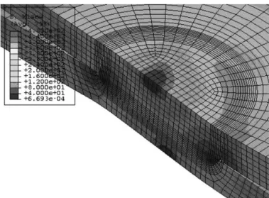
Theresultsobtainedfromsimulationshaveshownthatthe increase in the stress levels occurs predominantly around the contactsurfacebetweentheplates,asseeninFigure15tothe lap-shear test simulation.
Figure 15. Simulation image of the inal deformed shape of lap-shear specimen.
It is observed the stress distribution points to a progressive increase in the concentration of the higher stresses around the annular contact region between the two plates. The degree of elasticandplasticdistortionwassimilartothatobservedduring and after the actual experiments.
During simulation, as the load produced by the relative displacementbetweentheplatesisincreased,theregionofstress concentration is formed around the contact region as seen in the Figure 16.
Figure16.a)Stressdistributioninthecontactregionwhenthe maximum stress is close to r,
b) horizontal cut and c) vertical cut.
Figure 16-a shows that at the boundary of the contact region, the stresses reach their highest values. A horizontal cut throughoutthisregion(Figure16-b)showsthatanannularhigh stress region is formed. A vertical cut (Figure 16-c) conirms that
at this moment the stresses in the surroundings of this region are reasonablylow.
A further increase in load from this point increases the internal stresses which reach the material ultimate tensile strengthasseeninFigure17.Thespecimenfailuremodewill dependonhowthefracturedevelops.
FromFigure17theregionofhigherstressesextendstowards to the upper plate top surface, indicating a possible plug pull-out (Figure 18-a). This failure mode is associated to the combination of process parameters able to produce sound high resistance welds.
Figure17.Stressdistributionwhenσrisreached.
The through weld failure mode, shown in Figure 18-b, is associatedtolowloadcapacity.
Theresultsofthesimulationsperformedallowedtoidentify the plug pull-out failure mode. This behavior makes sense since the model exhibits no discontinuities as in the case of actual welds
It is worth to observe that the center of the stir zone has reachedverylowstressvalues,indicatingthatevencontaining a remaining hole as in the case of FSSW process, the joints can exhibit good mechanical properties.
Figure18.a)Plugpull-outandb)Through-weldinalfractureaspects[12].
Table 2. Welding parameters used to produce the test specimens, adapted from [16].
Welding condition
Shoulder plunge depth (mm)
Shoulder plunge rotational speed (rpm)
Shoulder retract rotational speed (rpm)
Maximum Force in lap-shear test
(kN)
1 0.2 2900 2700 7.0 ± 0.7
2 0.2 2400 2200 8.7 ± 0.6
3 0.2 1900 1700 6.7 ± 0.8
4 0.5 2900 2700 8.2 ± 1.7
5 0.5 2400 2200 8.8 ± 0.2
6 0.5 1900 1700 9.0 ± 1.9
The dimensions of the different joint regions (SZ, TMAZ and HAZshowninFigure5)weredeinedbasedintheactualvalues observedinajointproducedusingweldingconditionnumber6. Acomparisonbetweentheresultsofalap-sheartestperformed in a specimen welded at this condition and the test numerical simulationisshowninFigure19.Themaximumforceobtained from the simulation is very similar to the value attained during the actual test but the curve proile is different.
Sincenofailurecriterionhasbeenusedinthiswork,theshape of the simulation curve after the occurrence of yielding does not represents the actual behavior of the specimen. However, the numerical results obtained are coherent with the experimental values and allow to estimate the order of magnitude of joint strength,whencomparingdifferentjointgeometries.
The simulations performed in the cross-tensile model exhibit similar results. Figure 20 shows the distribution of stresses. The detail of the joint region presents a stress distribution very similar to that observed in the lap-shear simulation.
The presence of known discontinuities such as clad not homogeneously dissolved in the plates contact region can produce a change in failure mode from plug pull-out to through weldwithsigniicantdecreaseinjointresistance.Thissituation wasnotstudiedinthepresentwork.
Figure19.Comparisonbetweenexperimentalandnumerical resultsoflap-sheartestperformedinaweldjointobtained
Figure 20. Stress distribution during cross-tensile test simulation.Top–generalviewandbottom
–detailofplatescontactregion.
Conclusions 4.
Numerical models corresponding to lap-shear and cross-tensile test specimens were developed. The simulations have produced similar levels of stresses and distortions when comparedwithactualtestresults.
In the situations simulated, the stresses reached the ultimate tensile strength of material in an annular region around the joining area. Further increase in load extended this region towardstheupperplatetopsurfacecreatingaconditionwherea plug pull-out mode of fracture should occur.
Acknowledgements 5.
TheauthorswouldliketothanktheCAPES/DAADforthe PROBRAL program inancial support and to RIFTEC GmbH fortheproductionofweldedspecimens.
References 6.
[1] BENDZSAK, G. J., NORTH, T. H., LI, Z., Acta Metallurgica Materialia, 1997, 45 (4), p 1735-1745.
[2] CHAO, Y. J., QI, X., Heat Transfer and Thermo-Mechanical Analysis of Friction Stir Joining of AA6061-T6 Plates. Proceedings of the First International Symposium of Friction Stir Welding, 1999, Thousand Oaks, USA.
[3] COLEGROVE, P., Proceedings of the 2nd International Conference on Friction Stir Welding, 2nd ICFSW, Sweden 2000.
[4] XU, S., DENG, X., Two and Three-Dimensional Finite Element Models for the Friction Stir Welding , Park city, Utah, USA, May 14-16, 2003.
[5] ULYSSE, P., Three-dimensional Modeling of the Friction Stir-Welding Process, International Journal of Machine Tools & Manufacture 42 (2002) 1549-1557.
[6] ARBEGAST, W. J., Modeling friction stir joining as a metalworkingprocess,TMS,2003.
[7] SCHMIDT, H., HATTEL, J., WERT, J., Model. Simul. Mater. Sci. Eng. 2004, 12, 143-157
[8] MUCI-KUCHLER, K. H., ITAPU, S. K., ARBEGAST, W. J., KOCH, K. J.,VisualizationofMaterialFlowinFriction Stir Spot Welding, SAE paper: 2005-01-3323, V114-1, 2005 Transactions Journal of Aerospace.
[9] KALAGARA, S., MUCI-KüCHLER, K. H., Numerical Simulation of a Reill Friction Stir Spot Welding Process, Friction Stir Welding and Processing IV, TMS 2007, 369-378. [10] ITAPU, S. K., MUCI-KüCHLER, K.H., Visualization of MaterialFlowintheReillFrictionStirSpotWeldingProcess, SAE paper 2006-01-1206.
[11] ABAQUS/CAE User’s Manual, version 6.3, Hibbit, Karlsson & Sorensen, Inc, 2002.
[12] ROSENDO, T., SILVA, A. A. M., TIER, M. A. D., RAMOS, F. D., MAZZAFERRO, C. C. P., MAZZAFERRO, J. A. E., STROHAECKER, T. R., SANTOS, J.F., Preliminary Investigation on Friction Spot Welding of Alclad 2024 T3 Aluminium Alloy. XXXIII CONSOLDA - Congresso Nacional deSoldagem.CaxiasdoSul,27–30deAgostode2007. [13] TIER, M. A. D., SILVA, A. A. M., ROSENDO, T., MAZZAFERRO, J. A. E., MAZZAFERRO, C. C. P., RAMOS, F. D., STROHAECKER, T. R., SANTOS, J.F., Friction Based SpotWeldingProcesses–ALiteratureReview.Tobepublished, 159 pg., 2007.
[14] ROSENDO, T., SILVA, A. A. M., TIER, M. A. D., RAMOS, F. D., STROHAECKER, T. R., SANTOS, J. F., Friction Spot WeldingofAA2024T3AluminiumAlloy–AFeasibilityStudy. EUROMAT2007,Nuremberg,10th–13thSeptember2007. [15] SILVA, A. A. M., TIER, M. A. D., ROSENDO, T., RAMOS, F. D., MAZZAFERRO, C. C. P., MAZZAFERRO, J. A. E., STROHAECKER, T. R., SANTOS, J. F., Preliminary Investigations on Microstructural Features and Mechanical Performance of Friction Spot Welding of Aluminium Alloys. Proceedings of the IIW International Seminar on Friction based Spot Welding Processes. Geesthacht, 29th and 30th March 2007.
[16] SILVA, A. A. M, TIER, M. A. D., ROSENDO, T., RAMOS, F. D., MAZZAFERRO, C. C. P., MAZZAFERRO, J. A. E., STROHAECKER, T. R., SANTOS, J. F., Performance Evaluation of 2-mm Thick Alclad AA2024 T3 Aluminium Alloy Friction Spot Welding. SAE Aero Tech Congress Los Angeles, 17th–20thSeptember2007.
![Figure 2. Schematic illustration of the FSpW process variants [13].](https://thumb-eu.123doks.com/thumbv2/123dok_br/18858252.417445/3.892.155.727.78.1085/figure-schematic-illustration-fspw-process-variants.webp)
![Table 2. Welding parameters used to produce the test specimens, adapted from [16].](https://thumb-eu.123doks.com/thumbv2/123dok_br/18858252.417445/9.892.48.853.81.405/table-welding-parameters-used-produce-test-specimens-adapted.webp)

