Monitoring Biological Modes in a Bioreactor Process
by Computer Simulation
Samia Semcheddine1*, Abdel Aitouche2
1
Electronic Department, Faculty of Technology University of Setif UN1901
Cité Maabouda, Route de Béjaia 19000, Algeria E-mail: tssamia@ yahoo.fr
2
CRiSTAL UMR CNRS 9189, HEI
13 rue de Toul, 59046 Lille Cedex, France E-mail: [email protected]
*
Corresponding author
Received: June 22, 2015 Accepted: November 09, 2015
Published: December 22, 2015
Abstract: This paper deals with the general framework of fermentation system modeling and monitoring, focusing on the fermentation of Escherichia coli. Our main objective is to develop an algorithm for the online detection of acetate production during the culture of recombinant proteins. The analysis the fermentation process shows that it behaves like a hybrid dynamic system with commutation (since it can be represented by 5 nonlinear models). We present a strategy of fault detection based on residual generation for detecting the different actual biological modes. The residual generation is based on nonlinear analytical redundancy relations. The simulation results show that the several modes that are occulted during the bacteria cultivation can be detected by residuals using a nonlinear dynamic model and a reduced instrumentation.
Keywords: Monitoring, Fault detection, Residual generation, Biological modes, Escherichia coli.
Introduction
Genetically modified organisms are increasingly used in the pharmaceutical industry.
Escherichia coli, or E. coli, is still one of the most important host organisms used in the
pharmaceutical industry for producing recombinant proteins [2, 4, 12]. This paper aims to explore the possibility of monitoring changes in the metabolism of the E. coli during the fed-batch culture process [3]. Roeva and Tzonkov [9] used a heuristic procedure that employed dissolved oxygen probe measurements to distinguish two modes: acetate production or non-production by E. coli. This information is used to drive the feeding rate, and the global procedure is called probing control. A deeper analysis of the model used by [3] and [12] leads to five different metabolisms, which represent the modes of the E. coli cultivation.
[5]. Other approaches can be used, for example, observer-based approaches that reconstruct the process outputs, which are then compared to system measurements [7, 8].
All model-based fault detection methods have to generate residuals between the real behavior and the expected behavior, and some form of redundancy is needed to generate residuals. There are two types of redundancies: hardware redundancy and analytical redundancy. Hardware Redundancy (HR) using redundant sensors, for example has been applied in critical systems. Analytical Redundancy (AR) is obtained through a set of algebraic or differential relationships. The essence of AR in fault detection is to check the consistency of the real system behavior against the expected behavior of the system model. In this study, differential relationships were obtained using different sensor outputs and actuator inputs, and the residuals of these relationships were tested to identify the actual biological mode.
The contributions of this paper are:
- To detect biological modes by using approach of analytical redundancy instead of methods based on active control.
- This approach can be used to reduce the formation of acetate.
- The performances of the proposed approach are shown using the software Matlab – Simulink.
The paper is organized as follows. Section 2 provides a short description of the fed-batch fermentation process, which presents the hybrid structure of the process. Section 3 reports the results of our simulations using a nonlinear process model. Section 4 explains the concept of residual generation used to detect the actual biological mode, and Section 5 deals with the detection process applied to acetate production. Section 6 offers our conclusions and our perspectives for future research.
Process description
The fed-batch fermentation process considered in this study involves a genetically-modified
E. coli train that is cultivated in a bioreactor by using a probing control of fed batch
cultivations [3], by modeling E. coli using acetate inhibition [9]. The liquid medium contains cells and the substrates that are needed for the cell growth and production. The feed is used to control the substrate concentration. Air is transferred into the liquid in order to supply the culture with oxygen, with a mechanical stirrer agitating the liquid to insure that the air is well mixed with the liquid. A stirrer speed N is used to control oxygen transfer rate. Temperature and pH are maintained within operating conditions. Cell metabolism is described by the specific rates of growth, glucose uptake, oxygen uptake and net acetate production [4]. The model equations include these rates derived from mass balance in the liquid medium are:
*
,
,
,
in g
o
La o o o o
a
dX F
G A X X
dt V
dG F F
G G q G X
dt V V
dC F
K N C C C q G A X
dt V
dA F
q G A X A
dt V
where V, X, G, A, and Co are respectively the liquid volume, the cell concentration, the
glucose concentration, the acetate concentration and the dissolved oxygen concentration;
F, Gin and Co* denote respectively the feed rate, the glucose concentration in the feed, and the
dissolved oxygen concentration in equilibrium with the oxygen in gas bubbles; and KLa is the
volumetric oxygen transfer coefficient. V represents the volume variation.
In practice, most sensors do not measure the oxygen concentration but the dissolved oxygen
tension, which is related to the dissolved oxygen concentration through Henry’s law:
o
OHC
where Ois the oxygen concentrationandH is Henry’s constant and its value is 14103(l%)/g,
O* is the equilibrium dissolved oxygen tension and its value is 100%.
As mentioned in the last paragraph, cell metabolism is described by the specific rates of growth μ, glucose uptake qg, oxygen uptake qo and net acetate production qa [3].
The volumetric oxygen transfer coefficient KLa depends on the stirrer speed N and was
approximated using the following linear expression [1].
0
La
K N NN (2)
For the 3-liter laboratory bioreactor, 0.95 h-1·rpm and N0 = 323 rpm give a good
approximation for stirrer speeds between 400 rpm to 1200 rpm. These values were obtained using the KLa estimation technique suggested by [1].
The model given in System (1) depends on the specific rates mentioned above. The specific rate of growth is given by:
if
if
ox c crit
g m xg a xa g g
crit ox crit fe crit
g m xg g g xg g g
q q Y q Y q g
q q Y q q Y q g
(3)
where Yxgox is the oxidative biomass/glucose yield and its value is 0.51 g/g, fe xg
Y is the
fermentative biomass/glucose yield and its value is 0.15 g/g, Yxa is the biomass/acetate yield and its value is 0.40 g/g, crit
g
q is the critical specific glucose uptake rate and its value is
0.63 g/(gh).
The glucose consumed by the cells provides energy and raw material for the cell growth. The specific glucose uptake rate qg is assumed to be Monod-type:
maxg g
s
G
q G q
k G
(4)
where qmaxg is the maximum specific glucose uptake rate and its value is 1.0 g/(gh), ks is the
A part of the glucose uptake qg is assumed to be required for the non-growth associated to
maintenance. This is modeled by the flux, qm min q
g,qmc
, where qmc is the maintenance coefficient and its value is 0.06 g/(gh).The oxygen uptake qo is given by:
max
if
if crit g
c crit
g m og m om a oa g g
o crit
o g m og m om g q
q q Y q Y q Y q q
q
q q q Y q Y q
(5)
where Yog is the oxygen/glucose yield for growth and its value is 0.50 g/g, Yom is the oxygen/glucose yield for maintenance and its value is 1.07 g/g, Yoa is the oxygen/acetate yield and its value is 0.55 g/g.
The net acetate production is expressed by qa qapqac, where qap and qac denote respectively acetate production and consumption. The mathematical expression used for qac is:
,
, if
0 if
max
o g m og m om
c pot crit
a g g
c
oa a
crit
g g
q q q Y q Y
min q q q
Y q
q q
(6)
where
,
c max c pot a a
a
q A
q
k A
(7)
max o
q represents the maximum specific oxygen uptake rate and its value is 0.35 g/(gh),
c max a
q represents the maximum specific acetate consumption rate and its value is 0.20 g/(gh),
a
k is the saturation constant for acetate uptake and its value is 0.05 g/l.
The mathematical expression used for qap is:
if0 if
crit crit
g g ag g g
p
a crit
g g
q q Y q q
q
q q
(8)
ag
Y designs acetate/glucose yield and its value is 0.55 g/g.
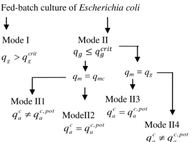
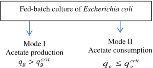
The metabolic relations show that the fed-batch fermentation process is a system with autonomous commutation, making it a hybrid dynamic system. According to the metabolic relations cited above, there are two modes. The first mode corresponds to qg qgcrit and is denoted “mode I”; the second mode corresponds to crit
g g
Fig. 1 shows the different situations that can arise in an E. coli culture, with one case for mode I and four cases for mode II.
Fig. 1 The different situations those can arise in an E. coli culture
Simulation of the process
We simulated a dynamic model of glucose overflow in fed-batch fermentation of E. coli
under fully aerobic conditions. The parameter used in this simulation for Gin is 60 g/l.
The initial values were: V(0) = 2.5 l, G(0) = 10 g/l, X(0) = 10 g/l, A(0) = 0 g/l and
O(0) = 30%. The Fig. 2 shows how we have chosen F. Our simulation results with the proposed model are shown in Fig. 3, Fig. 4 and Fig. 5. Fig. 3 shows that the fermentation process passes through 5 steps. We can interpret the first three phases from Fig. 4 and Fig. 5.
Fig. 2 Feed rate
Fig. 3 Biomass concentration
0 1 2 3 4 5 6 7 8 9 10
0 0.1 0.2 0.3 0.4 0.5 0.6 0.7 0.8 0.9
time(hours)
F
e
e
d
r
a
te
0 1 2 3 4 5 6 7 8 9 10
10 12 14 16 18 20 22
X: 7.941 Y: 21.16
time(hours)
c
o
n
c
e
n
tr
a
ti
o
n
(g
/l
X: 5.427 Y: 19.35
X: 3.412 Y: 16.28
X: 5.059 Y: 18.56
Mode I
crit g g q
q
Mode II
Mode II1
pot c a c a q q ,
qm = qg qm = qmc
Fed-batch culture of Escherichia coli
Mode II3
pot c a c a q
q ,
Mode II4
pot c a c a q q ,
ModeII2
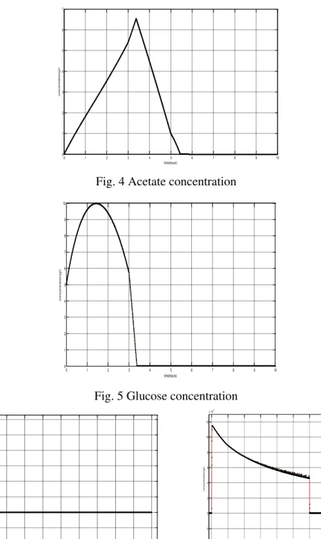
Fig. 4 Acetate concentration
Fig. 5 Glucose concentration
Fig. 6 Acetate and glucose concentration after 5 h
The supplied glucose leads to acetate production and good cell development (i.e., the biomass increases exponentially); when the glucose has been completely consumed, the biomass consumes the acetate to remain living, which leads to poor cell development. At about 5 h,
F is different of zero (Fig. 2) and therefore, the cell consumes glucose. The Fig. 4 also shows that at this moment, the slope of the acetate concentration curve increases slightly what proves that the presence of glucose leads to the production of acetate. But the curve remains decreasing what proves that the cell consumes acetate.
0 1 2 3 4 5 6 7 8 9 10
0 1 2 3 4 5 6 7
time(hours)
c
o
n
c
e
n
tr
a
ti
o
n
(g
/l
0 1 2 3 4 5 6 7 8 9 10
0 1 2 3 4 5 6 7 8 9 10
time(hours)
c
o
n
c
e
n
t
r
a
t
io
n
(
g
/
l
5 5.5 6 6.5 7 7.5 8 8.5 9 9.5 10 -0.2
0 0.2 0.4 0.6 0.8 1 1.2
time(hours)
c
o
n
c
e
n
tr
a
ti
o
n
(g
/l
5 5.5 6 6.5 7 7.5 8 8.5 9 9.5 10 -2
0 2 4 6 8 10 12 x 10-3
time(hours)
c
o
n
c
e
n
tr
a
t
io
n
(
g
/
To interpret the last two phases, we must show Fig. 6 that describes acetate and glucose concentration after 5 h.
When acetate is completely consumed, the biomass consumes glucose only; when acetate and glucose are completely consumed, the biomass stops developing.
The question that could be asked is at what mode is the process as was noted in the description of the hybrid dynamic system? The answer to this question is given in the following section, which presents residual generation as a method for detecting the modes of a biological system.
Residual generation
The method of residual generation is often used to detect the failure in automated systems. From a system model, it is possible to generate signals, called residuals, which are theoretically close to zero under normal operating conditions and not equal to zero when a failure occurs. Residuals can be also used in the context of a dynamic process whose evolution passes through several modes.
The evaluation procedure for redundancy relations given by the system model is based on elimination theory [10]. Two sensors are used to measure the glucose concentration (G) and the acetate concentration (A). In this case, the biomass X is deduced by using the second equation in the System (1), yielding:
s
in max
g
k G F F dG
X G G
q G V V dt
(9)
Then, the biomass X can be estimated by measuring the glucose concentration G.
The redundancy relations can also be obtained using the system model, by eliminating the unknown variables in the model equations. Without losing the generality of this paper, we will show how the biomass residual can be obtained using the first equation of the System (1):
,
d X F
rX G A X X
dt V
(10)
, , 1 2 3crit ox max crit fe
g mc xg g g xg
s
max ox
g mc xg
s
c max
max ox a
g mc xg xa
s a
c max a
a
d X G
rIX q q Y X q q Y X
dt k G
d X F G
rII X X q q Y X
dt V k G
q A
d X F G
rII X X q q Y X Y X
dt V k G k A
d X A F
rII X q X
dt k A V
4 omax gmax oaxa
s
d X F G
rII X X q q Y X
dt V k G
(11)
Similarly, using the last equation in the System (1), the acetate residual can be obtained:
,
a
dA F
rA q G A X A
dt V
(12)
The acetate residual can thus be obtained for each mode. The expressions of these 5 residuals are given by the following equations:
, , 1 2 3 4 max crit g g s max max
o g mc og
om s mc oa oa c max a a c max a a max max
o g om
s oa
dA G F
rIA q q X A
dt k G V
G
q q q Y
k G q Y
dA F
rII A X X A
dt Y Y V
dA A F
rII A q X A
dt k A V
dA A F
rII A q X A
dt k A V
G
q q Y
k G
dA F
rII A X
dt Y
A
V (13)
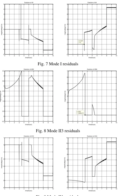
Fig. 8 shows that, after 3.4 hours, the 2 mode II3 residuals are null for a period which lasts until 5 hours, which corresponds to the acetate consumption. This consumption can be correlated with the decrease of acetate concentration (see Fig. 4).
Fig. 9 shows that, after 5 hours, the 2 mode II1 residuals are null for a period of less than half hour, which corresponds to the acetate consumption. This consumption can be correlated with the decrease of acetate concentration (see Fig. 4). In this mode, the acetate consumption related to goes to zero due to the lack of acetate. At the end of the fermentation process, mode II2 is active; the 2 residuals are null from 5.4 hours until 7.9 hours.
Fig. 7 Mode I residuals
Fig. 8 Mode II3 residuals
Fig. 9 Mode II1 residuals
0 1 2 3 4 5 6 7 8 9 10
-5 -4 -3 -2 -1 0 1 2 3 4 5 time(hours) m a g n it u d e (g /( l. h ))
Evolution of rIX
0 1 2 3 4 5 6 7 8 9 10
-2 -1 0 1 2 3 4 5 6 7 8 X: 3.337 Y: 0 time(hours) m a g n tu d e (g /( l. h ))
Evolution of rIA
0 1 2 3 4 5 6 7 8 9 10
-0.5 0 0.5 1 1.5 2 2.5 3 3.5 4 4.5 time(hours) m a g n it u d e (g /( l. h ))
Evolution of rII3X
0 1 2 3 4 5 6 7 8 9 10
-1 0 1 2 3 4 5 6 7 X: 3.541 Y: 3.929e-011 time(hours) m a g n it u d e (g /( l. h ))
Evolution of rII3A
0 1 2 3 4 5 6 7 8 9 10
-6 -5 -4 -3 -2 -1 0 1 time(hours) m a g n it u d e (g /( l. h ))
Evolution of rII1X
0 1 2 3 4 5 6 7 8 9 10
-4 -2 0 2 4 6 8 10 12 14 time(hours) m a g n it u d e (g /( l. h ))
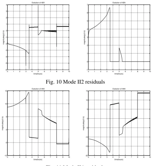
Fig. 10 Mode II2 residuals
Fig. 11 Mode II4 residuals
The 2 residuals are null from 5.4 hours until 8 hours (Fig. 8), mode II2 is active. In this mode, the glucose is limited, and acetate is no longer available.
Thus, the evolution of the mode II4 residuals (Fig. 11) is never close to zero. Thus, we can conclude that this mode is not reached by the process. We can also conclude that the simulation results shown in Fig. 7, Fig. 8, Fig. 9, Fig. 10, and Fig. 11 don not correspond to the results summarized in Fig. 1. To understand these phenomena, we must analyze the evolution of the specific glucose uptake and the acetate consumption, shown in Fig. 12.
Fig. 12 Evolution of qg qm and qacqc pota, over time
0 1 2 3 4 5 6 7 8 9 10
-6 -5 -4 -3 -2 -1 0 1 2 3 4 time(hours) m a g n it u d e (g /( l. h ))
Evolution of rII2X
0 1 2 3 4 5 6 7 8 9 10
-1 0 1 2 3 4 5 6 7 time(hours) m a g n it u d e (g /( l. h ))
Evolution of rII2A
0 1 2 3 4 5 6 7 8 9 10
-10 -5 0 5 10 15 time(hours) m a g n it u d e (g /( l. h ))
Evolution of rII4X
0 1 2 3 4 5 6 7 8 9 10
-20 -15 -10 -5 0 5 10 15 time(hours) m a g n it u d e (g /( l. h ))
Evolution of rII4A
0 1 2 3 4 5 6 7 8 9 10
-0.2 0 0.2 0.4 0.6 0.8 1 1.2 time(hours) m a g n it u d e (g /( g .h ))
Fig. 12 shows the temporal evolution of qg qm and qacqc pota, . In Fig. 1, the mode II4 is reached when qg qm is equal to zero and qacqac pot, is different to zero. But Fig. 12 shows that when temporal evolution of qg qm is nul then qacqac pot, is also null. The metabolic reaction does not fire modeII4. Thus, the residuals relating to this case is never null, as can be seen in Fig. 11. We deduced that the process does not really reach mode II4. We can thus conclude that the residual generation method can detect all the operating modes of the process, but only the modes represented in the Fig. 13 can be used.
Fig. 13 Various modes by which really the process passes
Detection of the acetate production mode
Acetate accumulation has been reported to inhibit growth and to reduce recombinant protein production. Thus, the interest of detecting this mode is quite obvious. In this section, we report the results of our experiments for detecting acetate production in a fed-batch culture of
E. coli.
According to the metabolic relations described above, there are two modes: the first mode corresponds to qg qgcrit and is denoted “mode I”; the second mode corresponds to qg qcritg
and is denoted “mode II”.
E. coli excretes acetate only when the specific glucose uptake rate exceeds the critical rate
(see Fig. 14), corresponding to a maximum respiration rate. The specific oxygen uptake rate
qo was initially fairly constant because
crit g
g q
q so, according to Eq. (8), qo qomax, but declined gradually as acetate accumulated.
Fig. 14 Modes related to acetate production and acetate production
Mode I Acetate production
Fed-batch culture of Escherichia coli
Mode II Acetate consumption
crit g g q q
Mode I
crit g g q
q
Mode II
crit g
g q
q
Mode II1
pot c a c a q
q , ModeII2
pot c a c a q q ,
Mode II3
pot c a c a q q ,
qm = qg qm = qmc
Two sensors were used to measure X and Co. qo was deduced using the last equation in
System (1), yielding:
*
,
o
La o o o
o
dC F
K C C C
V dt
q G A
X
(14)
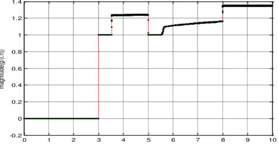
Fig. 15 represents the simulation of the residual generation, which can be expressed by the following equation
,
max
o o
rq q G A (15)
Fig. 15 Residuals related to acetate production detection
Fig. 15 shows that the acetate residual is null before 3 h. This residual was calculated from the available measurements, has to be close to zero when acetate production is detected. Compared to Fig. 15, our simulation results show that we can detect acetate production during the beginning of fermentation of a bacterium.
Conclusion
In the process of E. coli cultivation, which is a hybrid dynamic system, it is important to detect which kind of mode is active in the process in order to control it. Through our simulations results, this paper shows how the several modes that occur during the fermentation of bacteria can be detected (or not be detected) from the residuals generated from the nonlinear dynamic model of this process and a reduced instrumentation.
We first analyzed the process behavior, which shows that the process is a hybrid dynamic system with autonomous commutation. After this, we detect the different system modes. In order to detect the different modes, we used 2 sensors corresponding to acetate production and glucose uptake, and we showed that biomass, glucose and acetate can be estimated. We also showed that the residuals obtained, using the analytical redundancy approach, are able to detect the different process modes. Our results confirmed that the process reaches only four modes (acetate production, acetate consumption, acetate and glucose consumption and no acetate consumption) instead of all 5 modes. We also determined the exact period of the acetate production mode and the exact time that it takes place, which allows us to control the process.
0 1 2 3 4 5 6 7 8 9 10
-0.2 0 0.2 0.4 0.6 0.8 1 1.2 1.4
time(hours)
m
ag
ni
tu
de
(g
/(l
.h
For future research, we plan to investigate other detection approaches, such as the nonlinear observer approach. In order to reduce the cost of instrumentation, the idea is to use only one sensor, with which we have proved that the system remains observable: oxygen sensor. Indeed, this oxygen sensor is cheap and guarantees the sterility of environment.
References
1. Aitouche A., B. Ould-Bouamama (2010). Sensor Location with Respect to Fault Tolerance Properties, International Journal of Automation and Control, 4(3), 298-316. 2. Akesson M., P. Hagander (1999). A Gain-scheduling Approach for Control of Dissolved
Oxygen in Stirred Bioreactors, In: Preprints 14th world congress of IFAC, Chen et al. (Eds.), Vol. O, 505-510.
3. Akesson M., P. Hagander, J. P. Axelsson (2001). Probing Control of Fed-batch Cultivations: Analysis and Tuning, Control Engineering Practice, 9, 709-723.
4. Bastin G., D. Dochain (1990). On-line Estimation and Adaptive Control of Bioreactors, Amsterdam, New York, Elsevier.
5. Bouibed K., A. Aitouche, M. Bayart (2009). Nonlinear Parity Space Applied to an Autonomous Vehicle,Journal of Energy and Power Engineering, 3(12), 10-18.
6. Chow E. Y., A. S. Willsky(1984). Analytical Redundancy and the Design of Robust Failure Detection, IEEE Transactions on Automatic Control, 29(4), 603-615.
7. Edwards C., S. K. Spurgeon, R. J. Patton (2000). Sliding Mode Observers for Fault Detection and Isolation, Automatica, 36, 541-553.
8. Hammouri H., M. Kinnaert, E. H. El-Yaagoubi (1999). Observer-based Approach to Fault Detection and Isolation for Nonlinear Systems, IEEE Transactions on Automatic Control, 44(10), 1879-1884.
9. Roeva O., S. Tzonkov (2006). Modelling of Escherichia coli Cultivations: Acetate Inhibition in a Fed-batch Culture, International Journal of Bioautomation, 4, 1-11.
10. Semcheddine S., A. Aitouche, J. P. Cassar (2006). Detecting Modes in Fed-batch
Fermented Process. Application to Escherichia coli Cultivations, IMACS
Multiconference onComputational Engineering in Systems Applications, 1, 858-863. 11. Vant’Riet K. (1979). Review of Measuring Methods and Results in Nonviscous
Gas-liquid Mass Transfer in Stirred Vessels, Industrial and Engineering Chemistry Process Design and Development, 18(3), 357-364.
Assist. Prof. Samia Semcheddine, Ph.D. Student
E-mail: [email protected]
Samia Semcheddine was born on November 26, 1968 in Sétif, Algeria. She graduated from University of Sétif, Algeria in 2007. She became an Assistant Professor in the Department of Electronics at the University of Sétif, Algeria in 1998. She is currently a Ph.D. Student in Department of Electronics where she teaches course
“Automatic Materials”. Her research focuses on biotechnology.
Abdel Aitouche, Ph.D.
E-mail: [email protected]