ABSTRACT: The original radar cross section data or some rough models are often used to estimate a given aircraft target detection probability. The calculation results may not be very accurate as targets are different from one another and the real radar detection process is complex. A new method for radar cross section model generation is proposed and it takes the random factors like air turbulence into account; this makes it conform to the reality. In addition, this radar cross section model can be directly applied to the radar detection process to calculate the detection probability of a speciic aircraft at any attitude. Four typical aerial vehicles are taken as examples to demonstrate this method and information such as detection probability, signal to noise ratio and detection distance. Target’s instantaneous probability of being tracked, which corresponds to target’s detection probability, can also be calculated. Using these calculation results, we can compare two different aircrafts’ stealth performance in detail or optimize an aircraft’s light path.
KEYWORDS: Detection probability, RCS luctuation, Stealth performance, Aircraft target.
Calculation of Aircraft Target’s
Single-Pulse Detection Probability
Kuizhi Yue1,2, Shichun Chen2, Changyong Shu2
INTRODUCTION
It is a common practice that a radar cross section (RCS) of a target is interpreted as the target’s stealth performance or its detection probability by hostile radar. We all know that an aircrat with RCS value of σ = 0.1 m2 sounds better than
one with σ = 1 m2, but nobody can promise us that the irst
performs better than the latter in front of a really working radar, as radar detection process is probabilistic. he detection probability is inluenced by many random factors, such as the radar system’s parameters, the natural environment and most of all, as well as the RCS luctuation characteristic of the target. Radar system designers have utilized RCS fluctuation models to indicate a certain kind of targets for a long time. Plenty of researching work has been done and classical models like Swerling models, chi-square models etc. have been widely used (Shnidman 1995, 2005; Swerling 1960; Scholefield 1967). But all these models are meant to estimate a radar system’s detecting performance, not the stealth performance of an aircraft target. If those models are directly used on a specific aircraft, the process is somehow tedious and may cause great errors in model building (Johnston 1997).
However, we deinitely need to know the detection probability of a speciic aircrat. RCS is the fundamental parameter of an aircrat, whereas the detection probability is a parameter more important and intuitive. In a real combat situation, detection probability, along with target’s RCS luctuation characteristic, radar detection distance, false alarm probability, signal to noise ratio (SNR) etc. should all be taken into consideration. hese parameters can give us a more objective evaluation on the stealth performance of a specific aircraft. Researchers studying the optimal path planning for aerial vehicles are the representative ones who
1.Naval Aeronautical and Astronautical University – Department of Airborne Vehicle Engineering – Yantai – China. 2.Beihang University – School of Aeronautic Science and Engineering – Beijing – China.
Author for correspondence: Shichun Chen – Beihang University – School of Aeronautic Science and Engineering – Beijing 100191 – China | Email: [email protected]
care about real combat situations. When optimizing aircrat’s light path in a radar threatening situation, they need to know the stealth performance of the aircrat, as accurately as possible. A lot of literature about path planning has been published. heearly studies always treat the threatening radar as obstacles (Goerzen and Mettler 2010; Xu et al. 2010), which means the target’s detection probability is either 0 or 100%. Some researchers proposed aircrat’s dynamic RCS models which deal with RCS both in azimuth and bank angles (Moore 2002; Bortof 2000; Hebert 2001; Kim and Bang 2007), but they did not give any analysis on detection probability. Dogan (2003) and Wu et al. (2011) used probabilistic map to estimate the detection probability; the map is deined as the risk of exposure to the radar threats. And the risk is a function of target’s position. But this map is rough and cannot represent a speciic target accurately. Misovec et al. (2003) and Inanc and Muezzinoglu (2008) built a detection model using two diferent tables, which contain some parameters about the aircrat as well as the radar system. hey also gave an approximation function to express the detection probability. Parameters in both tables are also very general and only represent a certain kind of targets; when dealing with a speciic aircrat, they may bring unexpected errors. A popular model for calculating the target’s detection proba- bility was irstly proposed in Zeitz’s doctoral dissertation (Zeitz 2005). He derived an approximation function of target’s instantane- ous probability of being tracked. Many researchers prefer to use his function to calculate the aircrat’s probability of being tracked and then optimize the aircrat’s light path based on the calculation results (Ding et al. 2008; Liu et al. 2012; Mo et al. 2014; Kabamba
et al. 2006). his function considers many variables such as target’s RCS values, false alarm probability, SNR and radar system’s working settings. It also has a precise approximation expression, so it can give an accurate detection probability for any given RCS data.
he purpose of this paper is not to develop a new or improve an old path planning method. We focus on the aircrat’s stealth performance evaluation, from the perspective of detection probability. he calculation results will be useful if we want to know a speciic aircrat’s stealth performance in a real combat situation, and they can also be used in path planning optimizations.
SINGLE-PULSE DETECTION
PROBABILITY OF RCS FLUCTUATING
ZEITZ’S FUNCTIONAs Zeitz’s function is efficient in detection probability calculation and is widely used in estimating aircrat’s stealth
performance, we will analyze his function in this subsection. he irst variable in his function is the SNR, as deined in Eq. 1:
where:
Sr is SNR; σ is target’s RCS; R is the distance between radar and target; and K is a constant indicating radar system’s processing ability.
In fact, this equation is the derivation of the basic radar equation and no probabilistic variable is involved here.
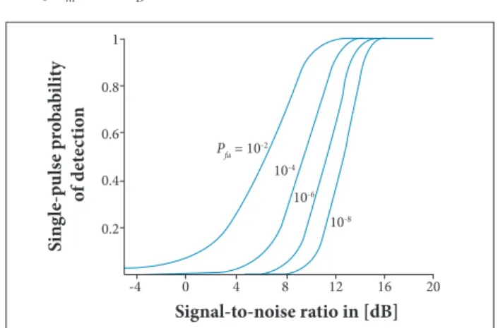
he second variable is the detection probability, PD, expressed as a function of SNR and false alarm probability, Pfa, as shown in Fig. 1 (Zeitz 2005).
This figure actually shows the single pulse detection probability of a signal with unknown phase but known amplitude (Difanco and Rubin 1968). he analytical expression of PD can be written as:
where:
rb is the detection threshold; r is an intermediate variable;
Sris SNR; and I0 is the modiied Bessel function of the irst kind and order zero.
The SNR here can be expressed as Eq. 3 and it has no matter with Eq. 1.
where:
E is the signal energy and N0/2 isthe two-sided white Gaussian noise spectual density. Sr here is equal to the ratio of maximum instantaneous signal power to average noise power out of a matched ilter (Difanco and Rubin 1968), and SNR in Zeitz (2005) is equal to the ratio of average instantaneous power to average noise power. So there exists a 3 dB discrepancy between igures drawn by Eq. 2 and Fig. 1, when Pfa value keeps the same. hen a probability of track loss, z[n], is deined as a recursion expression:
(1)
(2)
(3)
Single
pulse
r Matched
filter
Envelope
detector Sampling Threshold Yes
No where:
n is the transmitting pulses number and l is the consecutive misses number, being n > l and l > 2; Pm is the missing probability, being Pm = 1 – PD.
he instantaneous probability of being tracked, Ptrack, can then be expressed as Eq. 5 and its approximation function can be expressed as Eq. 6. he average probability of being tracked during a time interval, ΔT, can be expressed as Eq. 7.
Figure 2. Optimum detector for a single pulse. BASIC STEPS OF DETECTION PROBABILITY CALCULATION
A simpliied optimum detector for a single pulse of known amplitude and unknown phase can be illustrated in Fig. 2 (Difanco and Rubin 1968).
When the target is absent, the probability density function (PDF) of the intermediate variable, r, can be expressed as Eq. 8. his intermediate variable, r, is the output of a typical radar receiver’s envelope detector.
And, according to its deinition, the false alarm probability can be expressed as:
If the Pfa value is given, the threshold can be solved by Eq. (9) and expressed as:
When the target is present, the PDF of r can be expressed as:
-4 0
0 .2 0 .4 0 .6
Pfa = 10 -2
10-4
10-6
10-8 0.8
1
4 8 12 16 20
S
in
g
le
-p
u
ls
e p
ro
b
ab
il
it
y
o
f d
et
ec
ti
o
n
S i g n a l - t o - n o i s e r a t i o i n [ d B ]
Figure 1. Detection probability versus SNR and false alarm probability.
hen the detection probability, PD, can be expressed as Eq. 2. When target’s RCS luctuation characteristic is taken into considera-tion, the amplitude of the back scattering pulse changes with RCS. Equation 2 should be averaged with respect to amplitude statistics as:
(8)
(9)
(10) (5)
(6)
(7)
(11)
(12) where:
c1 and c2 are radar constants; t is time; τ is the time increment. Equations 4 and 5 combine Ptrack and PD. Equation 6 uses Eq. 1 as its SNR variable to connect Ptrack, R and σ, though the theoretical SNR should be Eq. 3. his substitution of SNR may cause extra calculation error.
PD in Eq. 2 is derived on assumption that the amplitude of the signal to be detected is already known, which means the target’s RCS value is a known constant in this equation, andno matter how many pulses are transmitted, the back scattering pulses will keep the same amplitude. his assumption does not take the RCS luctuation characteristic into account, which may bring some errors in PD calculation and in the following
where;
A is the back scattering pulse amplitude; p(A) is the PDF of A. When the RCS data of the aircrat target is known, p(A) can be obtained using the simple Eq. 13:
method described here can also be applied to RCS data obtained both in azimuth and elevation angles.
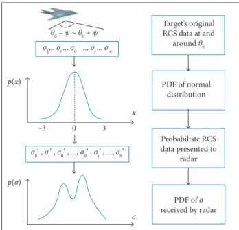
Figure 3 shows the framework of target’s RCS model generation: σ0 of the original RCS data corresponds to the azimuth angle θ0; σi (i = 1, 2, …, m) corresponds to an azimuth angle θi; θi is from an azimuth angle domain, θ0 – Ψ ~ θ0 + Ψ, whose center is at θ0, and θi is diferent from θ0; m + 1 is the total number of RCS values in this angle domain. his domain should be small enough if the aircraft flies relatively steadily. It is intentionally exaggeratedly drawn in Fig. 3 just for convenience.
Target’s original RCS data at and
around θ 0
PDF of normal distribution
Probabilistc RCS data presented to
radar
PDF of σ received by radar σ 0’ , σ i’ , σ 0’ , ..., σ 0’ , σ j’ , ..., σ 0’
σ 1... σ i ... σ 0 ... σ j ... σ m
p (σ )
σ
p (x )
-3 0 3
θ0 – ψ ~ θ 0 + ψ
x
Figure 3. Framework of RCS model generation.
he normal distribution in Fig. 3 is the one-dimensional normal distribution. he expectation value of x in the normal distribution is set to be 0, and the standard deviation is set to be 1. Both set values will not inluence the calculation results because what matters is the probability value of x, not the value of x itself. So the distribution can be expressed as:
Equation 14 can be used to generate a series of random values of x. Each x value corresponds to a speciic angle value and, consequently, a specific RCS value. The range of x in Eq. 14 is limited to be –3 ~ 3 because p(x) decreases to nearly 0 beyond x = ± 3. So the curve of p(x) can be truncated at x = ± 3; this means x = ± 3 exactly corresponds to the two extremes of the (14) (13)
where:
a is a constant depending on radar system’s working
parameters, such as transmitting power, antenna gain etc., and the distance R.
Radar experts prefer to use a fluctuation model, like a Swerling model, in Eq. 12 to estimate the radar system’s detecting performance when facing a “Swerling” target. If we want to know a speciic aircrat’s detection probability, we can directly use the discrete RCS data of the aircrat to generate a p(A) and substitute it into Eq. 12 to obtain target’s single pulse detection probability. his method can give a more accurate PD.
DETECTION PROBABILITY OF A
SPECIFIC AIRCRAFT
TARGET’S RCS MODEL GENERATION
When radar experts use classical luctuation models to analyze radar system’s performance, they do not need to know the exact attitude domain of the target. When aerospace experts use approximation models to analyze a speciic aircrat’s detection probability, they always assume that every attitude angle of the target has an equal probability of being presented to the radar (Robinson 1992; David 2007). his assumption is not always the reality and will bring some trouble in PD calculation accuracy. Our purpose is to calculate the PD of a speciic aircrat at a given angle θ0. We need to know the RCS value corresponding to that given angle as well as other RCS values around that angle, because an aircrat in light will always experience turbulence and other micro motions, and target’s RCS varies dramatically even with a small change in attitude (Paterson 1999). Taking into account these random factors, we assume that these RCS values obey the normal distribution when presented to the radar.
azimuth angle domain, respectively. he extremes are set to be θ1 and θm, and their corresponding RCS values are σ1 and σm. he “normrnd” function of MATLAB can be used to conduct this random process and generate a series of x values which obey the normal distribution. Using these x values, a series of RCS values can be obtained from the corresponding angle domain, as shown in the third frame of Fig. 3. hese probabilistic RCS values presented to the radar are much diferent from the original one. σ0 may appear much more times than σi. And the PDF of these random RCS values is diferent from that of the original ones. his PDF can then be used to calculate PD.
he variable presented in Fig. 3 is σ ; when applied to numerical calculation, the variable A is preferred, the derivation is the same as that of σ, and Eq. 13 can be used to obtain p(A) conveniently.
NUMERICAL CALCULATIONS AND ANALYSIS
In order to demonstrate our method, we choose four diferent types of aerial vehicles and obtain their RCS data by self-programmed sotware which is based on the physical optics (PO), equivalent current method (ECM), physical theory of difraction (PTD) and shooting and bouncing ray method (SBR). here are unavoidable errors in the RCS simulation results and we can never know the real RCS of a real aircrat like F-117A. However, our purpose is not to get an accurate RCS value of a target; we care more about target’s RCS luctuation characteristic and this self-programmed sotware can give a satisfactory prediction about target’s RCS luctuation trend.
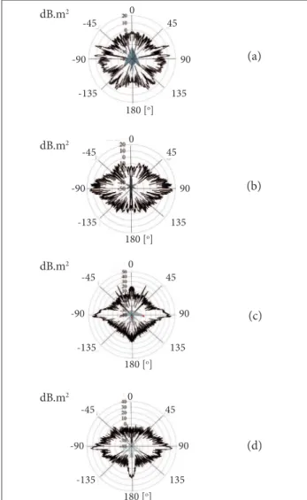
Figure 4 shows the RCS calculation mockups. SDM means self-designed missile. It is just an imaginary one and can be classiied as a stealth vehicle like F-117A as it obeys the basic stealth designing principles. X-21 is a big and conventional aircrat manufactured by Northrop and F-16 is a small and conventional aircrat.
RCS calculation is conducted at L band, which is oten used in ground-based searching radars (Paterson 1999). he polarization direction is horizontal. he calculation angle interval is 0.1°. he azimuth angle domain is set to be θ0 – 3° ~ θ0 + 3°. Figure 5 shows the RCS values of these four targets. θ = 0° corresponds to each target’s head direction. We can see that F-117A and SDM have comparably small RCS values; most of their RCS values are smaller than 0 dB.m2. X-21 and F-16 have
higher RCS values; most of their RCS values are much higher than 0 dB.m2. Figure 5 cannot tell us the speciic detection
probability, method mentioned in the previous sections can be used to obtain a speciic detection probability.
Firstly, Monte-Carlo (MC) method is used to generate the PDF of the back scattering pulse’s amplitude. he irst step is to generate a series of random values using “normrnd” function,
(a) F-117A (b) SDM
(d) F-16
(c) X-2 1
dB.m2 0
45
90
135
-4 5
-90
-135
18 0 [o]
0
45
90
135
-4 5
-90
-135
180 [o]
0 45
90
135 -45
-90
-135
180 [o]
0 45
90
135 -45
-90
-135
180 [o]
dB.m2
dB.m2
dB.m2
Figure 4. RCS calculation mockups.
Figure 5. Targets’ RCS polar curves. (a) F-117A; (b) SDM; (c) X-21; (d) F-16.
as described in the previous section. his function should be run enough times to generate enough x values to cover the whole range of –3 ~ 3 and, consequently, the whole range of
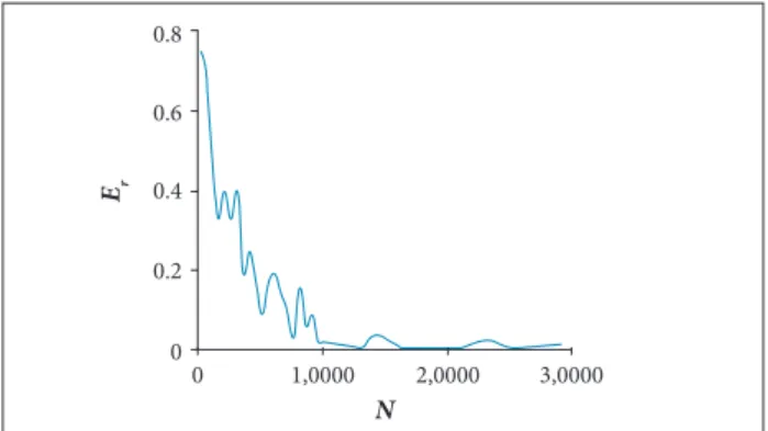
θ0– 3° ~ θ0+ 3°. We have conducted a lot of calculations, and the empirical repeating times for “normrnd” function is about 10,000 ~ 15,000. hen a steady PDF of these RCS values can be obtained, and this PDF can be used in Eq. 12 to obtain PD corresponding to the azimuth angle of θ0.
Figure 6 shows the inluence of repeating times, N, on the PDF curve’s steadiness. Er indicates the diference between the PDF of N = 20,000 and the PDF when N ≠ 20,000. It is
shown that when N exceeds about 10,000, the difference
between 2 PDF curves is very small. he RCS data used here is from the azimuth angle domain 64° ~ 70° of F-117A, but the conclusion is correct when the target or angle domain changes.
Er is deined in Eq. 15:
in RCS data range. his will lead to a diference in PD values. In this case, when the random process is considered, the result is
PD = 0.45 and when random process is not considered, PD = 0.53. SNR is about 14 dB and false alarm probability Pfa = 10-6, for both cases. If PD = 0.50 is the threshold to declare a single pulse detection, these 2 PDFs will bring diferent conclusions.
Figure 8 shows the relationship between SNR and PD for the conventional target X-21 and the stealth missile SDM.
θ = 0° corresponds to the head direction. PD generally changes with SNR. he PD of X-21 can always exceed 0.5 in the head direction, normal direction of leading edge, fuselage side direction and tail direction. In other directions, its PD is very small. As to SDM, its PD can always keep an even smaller
Figure 6. Inluence of N on the PDF curve’s steadiness (data from F-117A).
N
Er
0 0 0.2 0.4 0.6 0.8
1,0000 2,0000 3,0000
σ [m2]
p
0 0.00 0.05 0.10 0.15 0.20 0.25 0.30 0.35 0.40
2 4 6 8 10 12 14
With random process Without random process
Wing’s leading edge
3 5 5 1 5
25 35 45
0.90
0.70
0.50
0.30
0.10 0.90
0.70
0.50
0.30
0.10
25
15
5
-5
0 30 60 90 120 150 180
0 30 60 90 120 150 180
S
NR [dB]
S
NR [dB] P
D
PD
θ[o]
θ[o]
SNR PD
Figure 7. PDFs of F-117A at θ0 = 67°, with and without random process.
Figure 8. Relationship between SNR and PD (Pfa = 10-6). (a) X-21; (b) SDM.
(15)
where:
pN is the PDF when N ≠ 20,000; p0 is the PDF when
N = 20,000; i (i = 1, 2, …, k) indicates the discrete point of the PDF curve.
When the random process is conducted, the PDF of the back scattering values may be very diferent from the original one. Figure 7 shows the PDF of RCS from the angle domain of 64° ~ 70° of F-117A. he solid line indicates PDF ater conducting random process on the original data and the dotted line indicates PDF without random process, which means every RCS value in the original data have an equal probability to be presented to the radar. Two PDF curves are diferent either in coniguration or
(a)
PD
0
45
90
135
180 [o] -135
-45
-90
0
45
90
135
180 [o] -135
-45
-90
PD
1.0R 1.3R 1.7R
value at all angles except those near the side direction. Radar
working parameters for both vehicles are the same and the normalized detection distance of X-21 is twice that of SDM. If the working parameters of hostile radar are known, we can calculate target’s detection probability at any given distance and we are able to obtain the exact values of PD, SNR, Pfa and R. We can also compare two diferent targets’ stealth performance in the same threatening situation. he calculation results can help a lot on optimizing a light path.
For a speciic target, if more data about PD, SNR, Pfa and
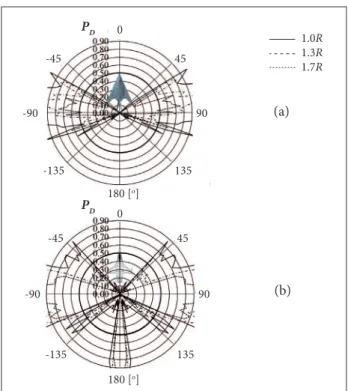
R are obtained, a complex polar curve can be drawn. Figure 9 gives an example for the stealth aircrat F-117A and conventional aircrat F-16. For each target, the radar is set to be at three diferent distances, with some certain working parameters. he detection distance R is normalized here because SNR varies with detection distance as well as radar transmitting power, radar antenna gain etc. If the transmitting power here is 200 W, the antenna gain is 30 dB, and other loss factors are set as common values; 1.0 R is about 15 km and the average SNR is about 15 ~ 20 dB. If the working parameters change, PD
will change but the coniguration and trend of its curve will not change too much.
Figure 9(a) shows that F-117A performs well in the direction between about θ = 0° ± 60°. his is an important angle domain to
a military aircrat. It also performs well in its tail direction between about θ = 180° ± 65°. PD in both domains is much smaller than 0.5 and the target can be regarded as perfectly stealthy. In the side direction between about 60° to 115°, F-117A performs not so well, PD can always exceed 0.5, but if the detection distance increases (so SNR decreases), PD will decrease fast synchronously in the whole angle domain.
Figure 9(b) shows that F-16 has a very low PD in the direction between about θ = 0° ± 40°. his sounds good but may not be the reality because the RCS calculation mockup of F-16 assumes that its cockpit and radar cabin have smooth surfaces from the perspective of electromagnetic. And RCS of its inlet may not be calculated accurately because of mockup’s simpliication. In fact, the real F-16 ighter plane does not have these smooth surfaces, cockpit and radar cabin are just 2 strongest RCS scatters on it.
PD in the tail direction is big because F-16’s nozzle does not have any stealth optimization measures. In the side direction between about 40°, which is just the normal direction of its wing’s leading edge, and 135°, F-16 has a very big PD, and if the detection distance increases (and SNR decreases), PD decreases not so dramatically and not synchronously, which is diferent from that of F-117A.
So, for a conventional aircrat like F-16 and a stealthy aircrat like F-117A, when they are close to a hostile radar, they perform almost the same from the perspective of detection probability. But when they get farther away from the radar, the diference becomes obvious; F-16 still keeps a high PD value in a broad azimuth angle domain, which means it can be easily detected. But the PD value of F-117A decreases fast in a broad angle domain, which means it gets undetected quickly.
he false alarm probability here is set to be Pfa = 10-6. If we
spend more time, we can draw a more complex figure for a speciic target, where PD varies with SNR, Pfa, and target’s attitude angle, like igures that oten appear in radar detection textbooks.
From Fig. 9 and the possible more complex igures, we can obtain very rich and relatively accurate information about a speciic aircrat’s stealth performance in front of threatening radars. his is the advantage of our method over other general detection models or basic RCS models.
hen we would like to discuss the instantaneous tracking probability, Ptrack, as mentioned in “Zeitz’s Function” section.
he appendix of Zeitz (2005) gives the detailed derivation of
Ptrack. It is a recursive expression and can be solved by recursive method. PD is assumed to be a constant here; l and n are system constants.
Figure 9. Target’s azimuth detection probability at different
distances (P
fa = 10-6). (a) F-117A; (b) F-16.
(a)
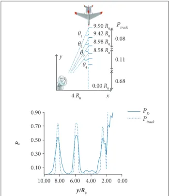
Figure 11. Target’s P
D and Ptrack in a simple combat situation
(n = 30, l = 5, P
fa = 10
-6).
We choose a simple but representative situation to demonstrate the calculation results. he target is lying from a longitudinal distance of y1 = 9.90 R0 towards the radar at a cross distance of
x0 = 4 R0 (R0 is a normalized distance). he azimuth angle between radar and target is θ1 = 22° when the target is at (x0, y1), and
yi (i = 2, 3, …, 69) is chosen to be 9.42 R0, 8.98 R0, 8.58 R0 etc. to make sure that their corresponding azimuth angles are θ2 = 23°,
θ3 = 24°,θ4 = 25°, until θ69 = 90°. PD,i and Ptrack,iare the detection and tracking probabilities at (x0, yi) (i = 1, 2, …, 69), and their curves are shown in Fig. 11. he peaks at about y = 7.8 R0 and
y = 6.0 R0 correspond to the normal directions of the wing’s leading edge and the horizontal tail’s leading edge, respectively. When X-21 is far from the radar, its PD and Ptrack are low, except the peaks. When it is close to the radar, its PD and Ptrack become higher due to a larger RCS value and a larger SNR.
The average value of being tracked during its flying time can be calculated based on the discrete Ptrack values. As
Δyi = y + 1 - y decreases with i, the integration time corresponding to each Ptrack,i (i = 1, 2, …, 69) decreases with i, if the target has a constant velocity. he light path is divided into 3 phases here for simplicity; each phase corresponds to a distance of 3.3 R0, and their average Ptrack values are 0.08, 0.11 and 0.68, respectively.
Equations 4 and 5 can be used to calculate a speciic target’s
Ptrack when PD is obtained. We can directly use those discrete PD
values in this equation, so does Pm. Each Ptrack corresponds to the same azimuth angle as PD.
Figure 10 is an example based on the data of Fig. 9. he detection distance is set to be a constant, R0. he radar system’s constants are n = 30 and l = 5; if we want to know more results,
R, n and l can be adjusted conveniently. Figure 10 shows that both aircrats’ Ptrack curves have nearly the same trend as their
PD curves in Fig. 9, and F-117A performs better almost in all directions, except in its leading edge’s normal direction. When the detection distance increases, the Ptrack of F-117A decreases fast and synchronously in the whole angle domain just as curves in Fig. 9(a). And the Ptrack of F-16 decreases not so dramatically and not synchronously when the detection distance increases, just as curves in Fig. 9(b).
Figure 10. Target’s instantaneous tracking probability in azimuth angle.
180[o]
-135 135
90 45 -45
0
Ptrack
-90
F -16 F-1 1 7 A
PD
Ptrack Ptrack
0.08
0.11
0.68
0.00 0.90
0.70
0.50
0.30
0.10
2.00 4.00 6.00 8.00 10.00
x y
4 R0
y/R0
P
θ1
θ2
θ4 8.98 R0 8.58 R0 9.42 R0 9.90 R0
0.00 R0
θ3
If we want to calculate the average tracking probability in a certain time interval, we just need to integrate the Ptrack values over the time interval and average the results, as shown in Eq. 7. Note that, in a speciic combat situation, target’s attitude angles may have diferent time periods of being presented to the radar, so the Ptrack values corresponding to each angle may be integrated with diferent time periods.
A CALCULATION EXAMPLE
CONCLUSIONS
e calculation of single pulse detection probability for
RCS luctuation targets has been analyzed and a new RCS model generation method has been proposed as the basis of the calculation. his method takes random factors like target’s micro motions and air low turbulence into account, so it conforms better to the reality. he RCS model can be directly used to calculate the detection probability of any speciic aircrat at any attitude. Some typical aerial vehicles are
taken as examples to illustrate this method. he instantaneous probability of being tracked has also been introduced and it can be calculated if the detection probability is obtained. By this method, the single pulse detection probability and instantaneous probability of being tracked for a speciic target can be calculated conveniently. Very rich information such as detection probability, false alarm probability, SNR, detection distance etc. can be obtained. Using this information, we can compare two diferent targets’ stealth performance or optimize a target’s light path.
REFERENCES
Bortoff SA (2000) Path planning for UAVs. Proceedings of the American Control Conference, American Automatic Control Council; Dayton, USA.
David KB (2007) Radar system analysis and modeling (in Chinese, translated by Nanjing Institute of Electronic Technology). Beijing: Publishing House of Electronics Industry.
Difanco JV, Rubin WL (1968) Radar detection. New Jersey: Prentice-Hall.
Ding XD, Liu Y, Li WM (2008) Dynamic RCS and real-time based analysis of method of UAV route planning (in Chinese). Systems Engineering and Electronics 30(5):868-871.
Dogan A (2003) Probabilistic approach in path planning for UAVs. Proceedings of the 2003 IEEE International Symposium on Intelligent Control; Houston, USA.
Goerzen C, Mettler ZKB (2010) A survey of motion planning algorithms from the perspective of autonomous UAV guidance. J Intell Robot Syst 57(1-4):65-100. doi: 10.1007/s10846-009-9383-1
Hebert JM (2001) Air vehicle path planning (PhD thesis). Wright-Patterson Air Force Base, Ohio: U.S. Air Force Institute of Technology.
Inanc T, Muezzinoglu MK (2008) Framework for low-observable trajectory generation in presence of multiple radars. J Guid Control Dynam 31(6):1740-1750. doi: 10.2514/1.35287
Johnston SL (1997) Target model pitfalls (illness, diagnosis, and prescription). IEEE T Aero Elec Sys 33(2): 715-720. doi: 10.1109/7.588498
Kabamba PT, Meerkov SM, Zeitz FH (2006) Optimal path planning for unmanned combat aerial vehicles to defeat radar tracking. J Guid Control Dynam 29(2):279-289. doi: 10.2514/1.14303
Kim BS, Bang H (2007) Optimal path planning for UAVs to reduce radar cross section. Int J Aeronautical & Space Sci 8(1):54-64. doi: 10.5139/ IJASS.2007.8.1.054
Liu HF, Chen SF, Zhang Y, Chen J (2012) Modelling radar tracking features and low observability motion planning for UCAV. Proceedings of the 4th International Conference on Intelligent Human-Machine System and Cybernetics; Nanchang, Jiangxi Province, China.
Misovec K, Inanc T, Wohletz J, Murray RM (2003) Low-observable nonlinear trajectory generation for unmanned air vehicles. Proceedings of the 42nd IEEE Conference on Decision and Control, Maui, Hawaii, USA.
Mo S, Huang J, Zheng Z, Liu W (2014) Stealth penetration path planning for stealth unmanned aerial vehicle based on improved rapidly-exploring-random-tree. Control Theory & Applications 31(3):375-385.
Moore FW (2002) Radar cross-section reduction via route planning and intelligent control. IEEE T Contr Syst T 10(5)::696-700. doi: 10.1109/ TCST.2002.801879
Paterson J (1999) Overview of low observable technology and its effects on combat aircraft survivability. J Aircraft 36(2):380-388. doi: 10.2514/2.2468
Robinson MC (1992) Radar cross section models for limited aspect angle windows (Master’s thesis). Montgomery: Air University.
Scholeield PHR (1967) Statistical aspects of ideal radar targets. Proceedings of the IEEE 55(4)::587-589. doi: 10.1109/PROC.1967.5610
Shnidman DA (1995) Radar detection probabilities and their calculation. IEEE T Aero Elec Sys 31(3):928-950. doi: 10.1109/7.395246
Shnidman DA (2005) Radar detection in clutter. IEEE T Aero Elec Sys 41(3):1056-1067. doi: 10.1109/TAES.2005.1541450
Swerling P (1960) Probability of detection for luctuating targets. IRE Transactions on Information Theory 6(2):269-308. doi: 10.1109/ TIT.1960.1057561
Wu SJ, Zheng Z, Cai KY (2011) Real-time path planning for unmanned aerial vehicles using behavior coordination and virtual goal (in Chinese). Control Theory & Applications 28(1):131-136.
Xu C, Duan H, Liu F (2010) Chaotic artiicial bee colony approach to uninhabited combat air vehicle (UCAV) path planning. Aerosp Sci Technol 14(8):535-541. doi: 10.1016/j.ast.2010.04.008