ALLOTMENT OF AIRCRAFT SPARE PARTS USING GENETIC ALGORITHMS
Pascale Batchoun
Département d'informatique et de recherche opérationnelle
Université de Montréal Montréal QC – Canada
Jacques A. Ferland *
Département d'informatique et de recherche opérationnelle
Université de Montréal Montréal QC – Canada [email protected]
Robert Cléroux
Département de mathématiques et de statistique Université de Montréal
Montréal QC – Canada
* Corresponding author / autor para quem as correspondências devem ser encaminhadas
Recebido em 04/2002, aceito em 11/2002 após 1 revisão
Abstract
In this paper we attempt to determine the optimal allocation of aircraft parts used as spares for replacement of defective parts on-board of a departing flight. In order to minimize the cost of delay caused by unexpected failure, Genetic algorithms (GAs) are used to allocate the initial quantity of parts among the airports. GAs are a class of adaptive search procedures, that distinguish themselves from other optimization techniques by the use of concepts from population genetics to guide the search. Problem-specific knowledge is incorporated into the problem and efficient parameters are identified and tested for the task of optimizing the allocation of parts. The approach is illustrated by numerical results.
1. Introduction
When a repairable item on an aircraft becomes defective, it is removed and replaced by another item from the spare stock. The defective part is then sent to the maintenance shop for repair. Should the station not have a spare part in stock, the aircraft will remain on ground and will be delayed until an incoming flight brings a replacement part from the maintenance shop or from a neighboring station. In this context, a repairable item represents any aircraft part from a small electronic component to a whole engine. Spare inventory is placed at line stations to decrease time delays due to unanticipated failures, and is placed also at the maintenance shop to quickly replenish remote station allotments while their parts are being repaired.
An agreement (“International Airlines Technical Pool”) between airlines exists to share certain parts at specific stations when parts fail. An airline is said to be the provider of a part at a specific station, when all the participant airlines of the agreement can borrow from the spare stock of the provider. In this case, a minimum of one part is allocated by the provider airline at that station.
A station is said to have maintenance ability for a certain part, when there is maintenance staff at the station accredited to remove and replace the defective part on the aircraft. When there is no maintenance ability for a specific part at a station, the aircraft with a defective part remains on ground until a technician flies into the station along with a replacement part. Therefore, the stations are given nil allotment for parts with no maintenance ability.
In this paper, we determine the optimal distribution of parts among the existing stations using a class of adaptive search procedures called genetic algorithms (GAs). The class of GAs distinguish themselves from other optimization techniques by the use of concepts from population genetics to guide the search. It would be difficult to use classical approaches based on exact algorithms since the economic function here is rather complex and thus requires much computational effort. Moreover, as will be seen below, an economic function has no particular structure that we could take advantage of in assessing the effect of slightly modifying a solution. When the number of spare parts is small an exhaustive search of the optimal solution can be made. But the solution space increases very quickly as the number of spare parts increases and consequently heuristic methods must be used. We chose to use genetic type methods to solve the problem. It will be seen that they yield good results and can be useful in some practical problems.
This problem is related to the mathematical model METRIC (Multi-Echelon Technique for
Recoverable Item Control). See for example Albright (1989), Demmy (1979), Demmy & Presutti (1981), Graves (1985), Muckstadt (1973, 1978), Muckstadt & Thomas (1980) and
Sherbrooke (1967). METRIC was designed for military application at the weapon-system
level where a particular item (part) may be demanded at several stations that are replenished
by one central depot. The major difference with our model is the fact that in the METRIC
model when an item becomes defective at a station, it can be replaced only by another item available at the station or at the central depot. Hence there is no lateral re-supply between
stations which we consider in our model. Tedone (1989) describes the RAPS (Rotables
Allocation and Planning System) system used by American Airlines and having similarities
with the METRIC system. In this approach, the spare parts are distributed among stations
The problem formulation is introduced in Section 2 as well as the failure process of parts and the evaluation of the delay associated with a given solution. Like some classes of algorithms, GAs include several parameters and strategies leading to several variants. In Section 3, the genetic algorithm implementation and its variations are described. Section 4 includes the numerical experiments to identify efficient parameters for optimizing the distribution of parts. A conclusion follows in Section 5.
2. Problem Formulation
A different problem is formulated for each type of part. The mathematical formulation of the problem for a specific type of part is quite straightforward, but the evaluation of the objective function is complex and time consuming.
2.1 Objective function and constraints
Assume that an initial quantity of N parts of a given type is available for redistribution among the stations and the maintenance shop for an airline. Denote
A: the set of line stations indices i (including the maintenance shop which is assumed to be located at one of the stations)
PP = { i∈ A \ the airline is the provider of the part type at station i}
PA = {i∈ A \ the airline is a participant to the pool at station i}
M = {i∈ A \ maintenance capacity exists for that part at station i}
M= A – M
Let S be the total number of stations operated by the airline: S = |A|. Let xi be the number of parts allocated to stations i ∈ A by the airline. The problem is to distribute the N parts among the S stations in order to minimize the expected cost of delay D = D(X) due to unexpected failures, where X = (x1, x2,…, xs). The problem then is to determine the optimal solution to the following optimization problem:
Minimize D(X)
s.t.
1 1 0 0 s
i i
i P
i A
i
x N
x i P
x i P
x i M
=
=
≥ ∀ ∈
= ∀ ∈
= ∀ ∈
∑
(2.1)
2.2 Evaluation of the cost of delay D(X)
In this section, we indicate how to determine the excepted cost of delay D(X) given a
2.2.1 Average cost of delay per removal
At station i, the total time delay δik due to the failure of a part prior to flight departure k includes the time to receive a serviceable part and the time to replace it on the aircraft. Since the replacement time of the part is constant regardless of the number of spares allocated at the station, it is not included in the time delay δik. Then if station i has a spare part to replace the unserviceable one at the time of failure, the time delay is nil. Otherwise, the time delay δik is the time it takes to receive a part through an incoming flight.
The flights considered in this study belong to a one week flight schedule. Consider the flight k, leaving from the origin station i. To determine the time delay δik in the case where no spare part is available at the time of failure on flight k, we take into account each flight io→i, leaving from origin station io, within 24 hours after the scheduled departure time of flight k, such that station io can provide a spare part. Denote δik(io) the time delay of flight k if the spare part is provided at station i by an incoming flight at station i and originating from station io.
Hence δik(io) is equal to the difference between the arrival time at i of this flight leaving from io and the schedule departure time of flight k.
To illustrate the evaluation process, consider the following time-space diagram where flights are illustrated with arcs:
t t
2 t1 t3 t4
i i
4
i
3
i
2
i
1
Time
Space
k
In this illustration, the flight leaving from i2 cannot bring a spare part because its departure
time is prior to the scheduled departure time of flight k. Furthermore, it follows that δik(ij) = tj –t for j = 1, 3,4.
Recall that our model is a planning tool to be used at the tactical level. Hence we do not
know precisely which station will have a spare part to provide station i prior to the
departure of flight k. Therefore we approximate δik using the following underestimate:
{
}
min ( ) 0
1440
o ik
ik o ik
i ik
i if
otherwise δ
δ = ∈Γ Γ ≠
(2.2)
where Γik= {io: io is the origin station of an incoming flight to i such that its departure time is within 24 hours after the scheduled departure time of k, and xio> 0 }. Here 1440
The average cost of delay di caused by the failure of a type of a part prior to any flight departure at station i is evaluated as follows:
1
0
ik A
k K i
A i P K
d
i P δ
∈
∀ ∉
=
∀ ∈
∑
(2.3)where K denotes the set of flights departing from station i during the week, and that are operated with an aircraft using a type of part.
2.2.2 Expected removals in a given period of time
The expected number of removals for a type of parts is the expected number of times a part fails during that time period. Based on historical data, the mean time between removals
(MTBR) τ, is the average number of flying hours between two successive removals. A type
of parts can belong to one or more types of aircraft. Let Q(u) be the quantity of parts belonging to the aircraft of type u. Let H(u) be the total hours operated by aircraft of type u during the week. Then the total expected number of removals λ for the part in a year is as follows:
( ) ( ) 52
. u
H u Q u
λ=
∑
∗τ ∗ (2.4)In order to calculate the expected number of removals per station during a year, let F(i,u) be the total number of flights per year with aircraft of type u, departing from station i. Then the total expected number of removals λi of that type of part at station i during a year is
( , ) ( )
,
( , ) ( )
λ
λ = ∗ ∗
∗
∑
∑ ∑
u i
i u
F i u Q u
F i u Q u
(2.5)
and
. i i
λ=
∑
λ2.2.3 Failure process
When failures of parts occur at a rate less than 10 per year, removals are assumed to follow a Poisson process. Since λ is the expected number of removals of the part during a year, the probability distribution of the number of removals kλt of the part in [0, t] is as follows:
0 !
( )
( ) ( ) .
!
t r
U U
t p t
r r
e t
P k U P k r
r λ
λ λ λ
=
≤ =
∑
= =∑
(2.6)Similarly, the probability distribution of the number of removals of the part at station i in [0, t] is
0
( )
( ) .
! i i
t r
V i t
r
e t
P k V
r λ
λ λ
−
=
When failures of the part occur at a rate greater than or equal to 10 per year (λ≥10), the number of removals in [0, t] is assumed to have a normal distribution with mean equal to λt and standard deviation σ= λt:
,
( ) .
N t N
U t
P kλ σ U P Z λ
σ−
≤ = ≤
(2.8)
2.2.4 Expected number of removals causing a delay
The variable xi denotes the initial number of spares allocated at station i. However this number is reduced whenever a spare part is being used. Let xi(t) be the number of spare parts available at time of failure t at station i:
xi(t) ≤xi ∀t. (2.9)
Two cases have to be considered to calculate the expected delay for station i according to the fact that xi = 0 or xi > 0.
If no spare part is allocated at station i then xi = xi(t) = 0, ∀ t. In this case, the expected number of removals at station i causing a delay is equal to the expected number of removals λi (see subsection 2.2.2) at station i.
If xi > 0, let µi be the expected number of removals at station i per year causing a delay. Note that xi≤λi, ∀i. Let µi(t) be the expected number of removals at station i during a time period t, causing a delay. Then given the allotment xi,
( ) 0 ( ) 1 ( 1) 2 ( 2)
i i i
i t P kλt xi P kλt xi P kλt xi
µ = ∗ ≤ + ∗ = + + ∗ = + …
( ) ( i )
i
i t
s x
s x P kλ s ∞
=
=
∑
− −( i ) ( i )
i i
t i t
s x s x
sP kλ s x P kλ s
∞ ∞
= =
=
∑
= −∑
=1 1
0 0
( ) 1 ( )
i i
i i
x x
i t i t
s s
t sP kλ s x P kλ s
λ − −
= =
= − = − − =
∑
∑
1
0
( ) ( ) ( )
i
i
x
i t i i
s
x s P kλ s x λt −
=
=
∑
− = − − (2.10)To evaluate µi we suppose that the stock runs out at station i during replenishment time R required to receive a serviceable part at the station from the shop in replacement of its unserviceable one. Now, R is equal to the transit time TT when the shop has spare part in stock. Otherwise, R = TT + TA where TA (Turn Around Time) is the time required to repair a defective part at the maintenance shop.
If we denote
( )
( ) 1
T
T A
P R T L
P R T T L
= =
it follows that the expected number of removals µi of the part causing a delay at station i is as follows:
[ ] (1 ) [ ]
µi= ∗L µi TT + −L µiTT +TA (2.11)
In order to simplify the computations, the expected number of removals at the shop (located at station M ) is taken to be equal to the total expected number of removals λ ( i)
i
λ=
∑
λ .The probability L is computed using the Poisson distribution function when λ < 10 or using the Normal distribution when λ≥ 10. Given the initial quantity of spare parts xD and the quantity of spare parts at the time of failure xM(t) at the shop, the probability L is given by
( M( )
L=P x t >0)=P R( =TT) (2.12)
and it is approximated by
( T D)
P kλ ≤x
that is the probability that the expected number of removals from the maintenance shop during the time required to repair a part is less than or equal to the number of spare parts at station M.
2.3 Average cost of delay
Let
0 0
1 0
i i
i if x J
if x >
= =
Then D(X), the expected total cost of delay caused by a failure given the allotment
1 2
( , , , s),
X = x x … x is as follows:
1
( ) ( (1 ) ).
s
i i i i i
i
D X d Jλ J µ
=
=
∑
+ − (2.13)It is worthy of note that we have to scan the weekly schedule file in order to evaluate the function D(X) for each solution X. Since the schedule may include a large number of flights, it follows that the evaluation of function D(X) is in general costly and computation-intensive to run.
3. Solution Approach Using Genetic Algorithms
expensive. Indeed, for a part with an allotment of N spare parts to be allocated at S feasible stations, the total number of possible solutions F(S, N) is as follows:
1 ( 1)!
( , ) .
!( 1)!
N S N S
F S N
N N S
+ −
+ −
= =
−
Hence if S = 15 and N = 6, then F(S, N) = 38,760, and if N increases to 11, the search space can be as large as 4,457,400 solutions.
Heuristic or approximate algorithms are often preferred in this case to quickly generate an approximate optimal solution. Genetic algorithms are population based heuristic techniques relying on the genetic inheritance, and allowing a more exhaustive search of the solution space. Some references on Genetic algorithms are the following: Buckles & Petry (1992), Davis (1987, 1991), Fox & Landi (1970), Goldberg (1989), Holland (1975) and Michalewicz (1992).
3.1 Presentation of the Algorithm
An initial population of n chromosomes or solutions is created. All n chromosomes are evaluated. At each generation, n chromosomes are chosen for reproduction from the current population. The selection is completed according to the proportional selection inducing a random process ensuring that the expected number of times a chromosome is chosen is approximately proportional to that chromosome’s performance relative to the rest of the population. Hence the same chromosome can be selected more than once. New chromosomes are generated by
means of genetic recombination operators. The recombination operator is called crossover,
and in general, it generates two new candidate solutions called offsprings. Then some
perturbations are applied to the offsprings with low frequency via the mutation operator. All the new offsprings are added to the set of parents to create a temporary population of size 2n.
n chromosomes are selected from the temporary population via proportional selection, to
create a new generation of size n. This process if repeated until a maximum number of
generations is reached. The genetic algorithm used in our study is summarized in Figure 1:
1. Create a temporary initial population of n chromosomes (Generation 0) 2. Evaluate the fitness of each chromosome
Repeat while the number of generations is less than the maximum number of generations:
3. Select n parents from the temporary population via proportional selection to create a new generation
Repeat until all parents are selected (n offsprings are created): 4. Choose a pair of parents for mating. Apply the crossover to create two offsprings
5. Process each offspring by the mutation operator End repeat
6. Evaluate the fitness of each offspring
7. Add the offsprings to the set of parents to form a new temporary population of size 2n
End repeat
3.2 Solution encoding
A crucial operation in using a genetic algorithm to solve a problem is the way of representing or encoding a solution. The technique for encoding a solution may vary from one problem to another. In earlier works, researchers used to encode all solutions as bit strings, regardless of the problem. Later, other types of encoding techniques were used. In our case, a bit string encoding is not natural. Indeed, a solution vector X = (x1, x2, …, xs) (the phenotype form of the solution) is encoded into a genotype form of dimension N, the initial number of spare parts. Each vector component contains the station index where one part is allocated. If more than one part is allocated at the station, then the station index is repeated for the next vector component. Denote G = (g1, g2, …, gN) the genotype representation of a vector solution, where gl∈A, l = 1, …, N, and A is a set of all stations. For example, for a part where N = 6 and S = 60, let X = (x1, x2, x3, …, xs) = (1, 0, 2, 0, …, 0, 3), the genotype vector G is represented as G = (1, 3, 3, 60, 60, 60).
The fitness of a chromosome solution G denoted as f(G), is defined to be the inverse of the cost of delay function D(X):
1
( ) .
( ) f G
D X =
3.3 Population
The population size n is the number of solutions or chromosomes per population. The
population size remains constant from generation to generation. Population size is a fundamental parameter of any GA. If the selected population size is too small, the algorithm may converge too quickly but not necessarily to a global or local optimal solution. On the other hand, a population with too many members offers a larger pool of diverse solutions, but might result in long waiting times for significant improvement.
The key feature of GAs is their ability to take advantage of the cumulated information about an initially unknown search space in order to bias subsequent search into useful subspaces. Most genetic algorithm implementations do begin with random populations. However, if problem-specific knowledge is available to indicate interesting regions of the feasible domain, then it should be used to guide the process. Initial solutions generated according to
problem specific-knowledge are called seeded solutions. Only the initial population is
seeded with good initial members.
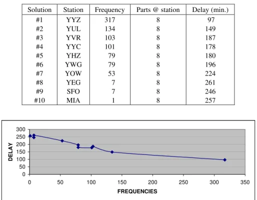
Table 1 – First situation: Seeded Solutions
Solution Station Frequency Parts @ station Delay (min.) #1 #2 #3 #4 #5 #6 #7 #8 #9 #10 YYZ YUL YVR YYC YHZ YWG YOW YEG SFO MIA 317 134 103 101 79 79 53 7 7 1 8 8 8 8 8 8 8 8 8 8 97 149 187 178 180 196 224 261 246 257 0 50 100 150 200 250 300
0 50 100 150 200 250 300 350
FREQUENCIES
DELAY
Figure 2 – First situation: Frequency-Delay Relationship
Since the time delay at a station does not depend uniquely on the number of spare parts but also on the providing from the neighboring stations, another situation is analyzed. Here, we use the same part with the same feasible stations, but we assume that 72 spare parts are available. Ten different solutions are evaluated where no spare part is assigned to one station and 8 spares to each of the other 9 stations. The results in Table 2 and Figure 3 indicate that, in general, the time delay increases with the augmenting of the departure frequency of the station having no spare part.
Table 2 – Second situation: Seeded Solutions
30 40 50 60 70
FREQUENCIES
DELAY
Figure 3 – Second situation: Frequency-Delay Relationship
Relying on these observations, the initial population can be partially seeded using frequency of departures per station as a parameter. In this case, some seeded chromosomes are included in the initial population. Each seeded chromosome is specified according to the following proportional selection process. First, the stations are ordered in some sequence. To determine the station in each position of the chromosome, a random positive integer smaller than or equal to the total number of flights is generated. Then we select the first station in the sequence such that the sum of its frequency and those of the previous stations in the sequence is greater than or equal to the random number. This proportional selection process ensures that the expected number of times a station is chosen is approximately proportional to that station frequency relative to the rest of the stations. Station indices per generated solution are sorted in ascending order, i.e. for an initial solution G = (g1, g2, …, gN), gl≤gm
∀l ≤m. In Section 4, numerical results are used to analyze the influence of the percentage of seeded solutions in the initial population and the effect of sorted initial solutions.
At each generation, n new parents are selected from the temporary population. Each new
parent is selected according to a proportional selection process, also known as the roulette wheel parent selection in order to ensure that the expected number of times a chromosome is chosen is approximately proportional to its performance relative to the rest of the population. First the fitness values of all chromosomes in the current population is determined and the chromosomes are ordered in some sequence. Then the following procedure is applied to determine each of the n parents:
1. Generate a random number between 0 and the total of the fitness values.
2. Select the first chromosome in the sequence whose fitness value added to the sum of the fitness values of the previous chromosomes in the sequence is greater than or equal to the random number generated at step 1.
As mentioned before, proportional selection process is applied to the temporary population formed by n parents and their n offsprings in order to form a new generation of n
chromosomes (with the exception of the temporary initial solution which contains only n
3.4 Operators
Crossover is an extremely important component of genetic algorithm. It is regarded as the distinguishing feature of GAs and as a critical accelerator of the search process. Crossover is a structured yet randomized information exchange between two chromosomes. The role of the crossover operator is to combine two solutions into an offspring that shares characteristics from both parents. The more widely used operators are the 1-point, the 2-point, and the uniform crossovers. Since in our problem the dimension of the vector solution varies between 3 and 11, only the 1-point and the uniform operators are compared.
In the 1-point crossover, we randomly select a cut point in the parents. Then offsprings are generated by combining the genetic material of one parent on the left-hand side of the cut point with that of the other parent for the positions on the right-hand side (and including the cut point). Figure 4 illustrates an example where two parents are combined via the 1-point crossover.
Parent 1 MIA SFO YEG YHZ YVR YWG YUL YUL YYZ
Parent 2 SFO YEG YHZ YWG YWG YUL YYZ YYZ YYZ
Random
Position ↑
Offspring 1 MIA SFO YEG YHZ YVR YUL YYZ YYZ YYZ
Offspring 2 SFO YEG YHZ YWG YWG YWG YUL YUL YYZ
Figure 4 – 1-point Crossover
In the uniform crossover operator, a random bit string of size N is generated. The station in each position of the offsprings is specified according to the bit string as follows: if there is a 0 in a given position of the bit string, the offspring 1 inherits the station of parent 2 for the same position, and offspring 2, that of parent 1. If there is a 1 instead, offspring 1 inherits the station of parent 1, and offspring 2, that of parent 2. Figure 5 illustrates the combination of two parents using a uniform crossover.
Mutation occurs after crossover is applied, but only a small percentage of the time. Indeed, with a 1% probability, every component of each vector solution is replaced by a random feasible station.
Parent 1 MIA SFO YEG YHZ YVR YWG YUL YUL YYZ
Parent 2 SFO YEG YHZ YWG YWG YUL YYZ YYZ YYZ
Random Bit
String 0 1 1 1 0 1 0 0 0
Offspring 1 SFO SFO YEG YHZ YWG YWG YYZ YYZ YYZ
Offspring 2 MIA YEG YHZ YWG YVR YUL YUL YUL YYZ
4. Numerical Results
Choosing a suitable population size, the right combination operator or even a reasonable stopping criteria are key decisions faced by all genetic algorithm users. Parameter settings greatly influence performance. Some of the parameters are tested individually and some dependent parameters are tested when combined. In order to test one parameter, all the others are fixed and the tested parameter is assigned various values.
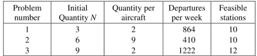
Three different problems with 3, 6 and 9 spare parts available are used to analyze the parameter values. Each part type belongs to a different aircraft type, but each fleet covers a similar network of stations. The number of parts per aircraft, the number of flight departures per week, and the number of feasible stations covered by the fleet type are summarized in Table 3.
Table 3 – Part types
Problem number
Initial Quantity N
Quantity per aircraft
Departures per week
Feasible stations 1
2 3
3 6 9
2 9 2
864 410 1222
10 10 12
For each test, each problem is solved 10 times. In the different tables summarizing the results, the “Best Value” column indicates the minimum cost of delay achieved among the total number of runs. The average cost of delay for the 10 tests is also indicated together with the confidence interval having a 95% confidence level. A confidence interval noted ±β corresponds to A(X) ± β, where A(X) is the average of the 100 tests. The tables also include the number of times (out of the 10 runs) that the best value is reached, the average number of solutions generated per test, and the average time of execution. Note that the computations were executed on a PC based Toshiba 4030 CDS, 233 MHz.
4.1 Stopping criteria
The stopping criterion used in our tests consists of stopping the process when the number of iterations reaches 10 ∗N/2, a number proportional to the number N of spare parts available for the problem. This stopping criterion results in exploring a reasonable number of solutions and obviously not exceeding the total number of feasible solutions.
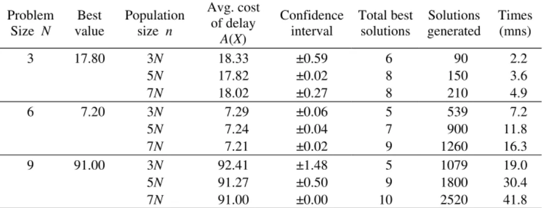
4.2 Population size
The population size n remains constant from generation to generation, and it is directly proportional to the length of the genotype vector N (the number of spare parts available):
n = αN, where α is a positive integer. Three different values of α are tested, and the results are summarized in Table 4. The parameters are fixed as follows:
Population size test: n = 3N or n = 5N or n = 7N (α = 3,5 or 7). Mutation operator rate: 1%
Percentage of best solutions for new generation: 10% Crossover operator: Uniform
Initial solutions are sorted: G = (g1, g2, …, gN), gl≤gm ∀l≤m.
As far as solution quality is concerned, the results are quite similar when α is equal to 3 and 5. However, the larger the population size, the more solutions are evaluated, and therefore solution time increases. Hence, the population size n = 5N is selected.
Table 4 – Population Size Test Results
Problem Size N
Best value
Population size n
Avg. cost of delay
A(X)
Confidence interval
Total best solutions
Solutions generated
Times (mns)
3 17.80 3N
5N
7N
18.33 17.82 18.02
±0.59 ±0.02 ±0.27
6 8 8
90 150 210
2.2 3.6 4.9 6 7.20 3N
5N
7N
7.29 7.24 7.21
±0.06 ±0.04 ±0.02
5 7 9
539 900 1260
7.2 11.8 16.3
9 91.00 3N
5N
7N
92.41 91.27 91.00
±1.48 ±0.50 ±0.00
5 9 10
1079 1800 2520
19.0 30.4 41.8
4.3 Seeded initial population
As it has been indicated in Section 3, the delay is inversely proportional to the departure frequency at the station when all spare parts are allocated to the same station. However, the presence of too many highly fit chromosomes in the initial population may result in premature termination at a local optimum. In order to identify the best strategy, three values are tested for the percentages of seeded initial solutions:
Percentage of seeded solutions in initial population: 20% or 50% or 80% Population size n = 5N
Mutation operator rate: 1%
Percentage of best solutions for new generation: 10% Crossover operator: Uniform
Initial solutions are sorted: G = (g1, g2, …, gN), gl≤gm ∀l≤m.
Table 5 – Initial Population Test Results
Problem Size N
Best value Seed percentage Avg. cost of delay
A(X)
Confidence interval Total best solutions Solutions generated Times (mns)
3 17.80 20% 50% 80% 18.29 17.80 18.23 ±0.50 ±0.00 ±0.41 5 10 7 176 150 160 5.2 4.3 4.7 6 7.20 20%
50% 80% 7.25 7.24 7.26 ±0.05 ±0.04 ±0.06 7 7 7 930 930 900 12.6 12.1 11.7 9 91.00 20%
50% 80% 91.47 91.27 91.24 ±0.48 ±0.50 ±0.30 7 9 8 1804 1804 1804 30.0 30.5 30.1
4.4 Parent selection
At each iteration, a small percentage of best performing chromosomes selected as parents at the preceding iteration is kept, and the others are selected according to proportional selection. The results for four different percentages are summarized in Table 6.
Percentage of best solutions: 0% or 4% or 10% or 25% Population size n =5 N
Mutation operator rate: 1%
Percentage of seeded solutions in initial population: 50% Crossover operator: Uniform
Initial solutions are sorted: G = (g1, g2, …, gN), gl≤gm ∀l≤m.
When the best performing solutions are not forced to remain from generation to generation (best solutions percentage = 0%), they tend to be lost. Hence, the results in Table 6 indicate that the algorithm takes longer to regenerate good performing solutions. However, when the percentage selection is 10% or 25%, the results for all 3 problem-tests are very good. For the problem when N = 3, a percentage selection of 25% seems to be a bit too aggressive as 3 out of 10 tests converge to a local minimum.
15.00 20.00 25.00 30.00 35.00 40.00 45.00
0 2 4 6 8 10
Generations
Cos
t of De
la
y
20% Seeded 50% Seeded 80% Seeded
4.5 Crossover operator
The uniform crossover and the 1-point crossover operators are compared. An additional component is added to the tests of the crossover operators in order to analyze the relevance of sorting the chromosomes in the initial solutions. Both parameters are tested jointly since the value of one can be dependent on the other. The results summarized in Table 7 are obtained using the following parameters:
Crossover operators: Uniform or 1-point.
Initial solutions are sorted: G = (g1, g2, …, gN), gl≤gm ∀l≤mor non-sorted. Percentage of best solutions: 10%
Population size n = 5N
Mutation operator rate: 1%
Percentage of seeded solutions in initial population: 50%
The results for problem 2 where N = 6 are not very conclusive, since the average values for the 4 combinations of the two parameters are very similar and the confidence intervals are short. Now, for the problems with N = 3 and N = 9, the results in Table 7, indicate that sorting the initial solutions (i.e. sorting the station indices within each chromosome) seems to allow generating better chromosomes and therefore the algorithm converges to better solutions.
Table 6 – Offsprings Selection Test Results
Problem Size N
Best value % Best solutions Avg. cost of delay
A(X)
Confidence interval Total best solutions Solutions generated Times (mns)
3 17.80 0% 4% 10% 25% 18.23 17.91 17.80 18.01 ±0.30 ±0.18 ±0.00 ±0.40 5 8 10 7 176 176 176 176 4.00 4.60 4.25 4.30
6 7.20 0% 4% 10% 25% 7.59 7.28 7.24 7.22 ±0.13 ±0.05 ±0.04 ±0.02 2 4 7 8 930 930 930 918 12.70 12.20 12.13 12.00
Table 7 – Crossover Test Results
Problem Size N
Best value Crossover operator Sorted initial solutions Avg. Cost of delay
A(X)
Confidence interval Total best solution Times (mns)
3 17.80 Uniform
1-Point Uniform 1-Point No No Yes Yes 18.06 17.92 17.80 17.93 ±0.26 ±0.33 ±0.00 ±0.33 4 8 10 7 4.50 4.10 4.25 4.60
6 7.20 Uniform 1-Point Uniform 1-Point No No Yes Yes 7.25 7.22 7.24 7.27 ±0.10 ±0.04 ±0.07 ±0.10 8 8 7 6 11.60 11.60 12.13 11.60
9 91.00 Uniform
1-Point Uniform 1-Point No No Yes Yes 94.71 92.02 91.27 91.36 ±0.77 ±1.28 ±0.50 ±0.55 7 5 9 7 30.30 30.90 30.50 31.50
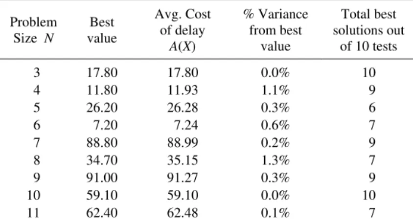
Table 8 – Test Results for Various Part Types
Problem Size N
Best value
Avg. Cost of delay
A(X)
% Variance from best
value
Total best solutions out
of 10 tests
3 4 5 6 7 8 9 10 11 17.80 11.80 26.20 7.20 88.80 34.70 91.00 59.10 62.40 17.80 11.93 26.28 7.24 88.99 35.15 91.27 59.10 62.48 0.0% 1.1% 0.3% 0.6% 0.2% 1.3% 0.3% 0.0% 0.1% 10 9 6 7 9 7 9 10 7
The uniform crossover is more efficient than the 1-point crossover in 5 out of 6 cases, as shown in the “Total Best Solutions” column. This result is consistent with the one obtained in Syswerda (1989) (Section 4.6).
4.6 Numerical results for 9 problems
5. Conclusion
Since the problem includes a small number of constraints, Genetic Algorithms seem to be very appropriate to deal with the Aircraft Spare Parts problem. The percentage variance of the average cost from the best value varies between 0.0% to 1.3%. This is the case for all problem sizes, for various part types and aircraft types.
It is worth noting that the algorithm is computation intensive to run. The evaluation of a solution is making the algorithm computationally expensive, as the delay is estimated for every single flight of the week. Should this optimization be required on a frequent basis, or within few hours, the cost of delay could be simulated instead of being fully evaluated. By doing so, the execution would be reduced.
Of course comparisons should be made with other approaches. But this would be the object of another paper.
Acknowledgements
This research was supported by NSERC grants OGP0003736 and OGP0008312.
The authors thank the referees for their helpful comments.
References
(1) Albright, S.C. (1989). An approximation to the Stationary Distribution of a Multiechelon Repairable Item Inventory System with Finite Sources and Repair Channels. Nav. Res. Logist. Quart., 36, 179-195.
(2) Buckles, B. & Petry, F. (1992). Genetic Algorithms. IEEE Computer Society Press, Los Alamitos, California.
(3) Cho, D.I. & Parlar, M. (1991). A Survey of Maintenance Models for Multi-Unit Systems. Euro. Jour. Oper. Res., 51, 1-23.
(4) Davis, L. (1987). Genetic Algorithms and Simulated Annealing. Pitman, London,
England.
(5) Davis, L. (1991). Handbook of Genetic Algorithms. ed., Van Nostrand Reinhold, New
York, New York.
(6) Demmy, W.S. (1979). On the METRIC Distribution Algorithm. Modeling and
Simulation, 10, 523-588.
(7) Demmy, W.S. & Presutti, V.J. (1981). Multi-Echelon Inventory Theory in the Air Force Logistics Command. TIMS Studies in the Management Sciences, 16, 279-297.
(8) Fox, B. & Landi, M. (1970). Searching for the Multiplier in One-Constraint Optimization Problems. Oper. Res., 18, 253-262.
(9) Goldberg, D.E. (1989). Genetic Algorithms in Search, Optimization, and Machine
(10) Graves, S.C. (1985). A Multi-Echelon Inventory Model for a Reparable Item for one Replinishment. Manag. Sci., 31, 1247-1256.
(11) Holland, J.H. (1975). Adaptation in Natural and Artificial Systems. University of
Michigan Press, Ann Arbor, Michigan.
(12) Kim, J.S.; Shin, K.C. & Park, S.K. (2000). An Optimal Algorithm for Repairable Item Inventory System with Depot Spares. Jour. Oper. Res. Soc., 51, 350-357.
(13) Michalewicz, Z. (1992). Genetic Algorithms + Data Structures = Evolution Programs.
Springer-Verlag.
(14) Muckstadt, J.A. (1973). A Model for a Multi-Item, Multi-Echelon, Multi-Indenture Inventory System. Manag. Sci., 20, 472-481.
(15) Muckstadt, J.A. (1978). Some Approximation in Multi-Item, Multi-Echelon Inventory Systems for Recoverable Items. Nav. Res. Logist. Quart., 35, 377-394.
(16) Muckstadt, J.A. & Thomas, L.J. (1980). Are Multi-Echelon Inventory Methods Worth
Implementing in Systems with Low Demand Rate Items? Manag. Sci., 26, 483-494.
(17) Sherbrooke, C.C. (1967). METRIC: Multi-Echelon Technique for Recoverable Item Control. Oper. Res., 16, 122-141.
(18) Syswerda, G. (1989). Uniform Crossover in Genetic Algorithms. Proceedings of the
Third International Conference on Genetic Algorithms, San Mateo, California, Morgan Kaufmann Publisher, 2-9
(19) Tedone, M.J. (1989). Reparable Part Management. Interfaces, 19(4), 61-68.
(20) Zorn, W.L.; Deckro, R.F. & Lehmkuhl, L.J. (1999). Modeling Diminishing Marginal Returns in a Hierarchical Inventory System of Repairable Spare Parts. Ann. Oper. Res.,