Comparation of logistic regression methods and discrete choice
model in the selection of habitats
Sandra Vergara Cardozo
1; Bryan Frederick John Manly
2; Carlos Tadeu dos Santos Dias
3*
1
Universidad Nacional de Colombia – Departamento Estadística – 111321 – Bogotá – Colombia. 2
Western EcoSystems Technology Inc., Cheyenne, WY 82001 – USA. 3
USP/ESALQ – Depto. de Ciências Exatas – C.P. 09 – 13418-900 – Piracicaba, SP – Brasil. *Corresponding author <ctsdias@esalq.usp.br>
ABSTRACT: Based on a review of most recent data analyses on resource selection by animals as well as on recent suggestions that indicate the lack of an unified statistical theory that shows how resource selection can be detected and measured, the authors suggest that the concept of resource selection function (RSF) can be the base for the development of a theory. The revision of discrete choice models (DCM) is suggested as an approximation to estimate the RSF when the choice of animal or groups of animals involves different sets of available resource units. The definition of RSF requires that the resource which is being studied consists of discrete units. The statistical method often used to estimate the RSF is the logistic regression but DCM can also be used. The theory of DCM has been well developed for the analysis of data sets involving choices of products by humans, but it can also be applicable to the choice of habitat by animals, with some modifications. The comparison of the logistic regression with the DCM for one choice is made because the coefficient estimates of the logistic regression model include an intercept, which are not presented by the DCM. The objective of this work was to compare the estimates of the RSF obtained by applying the logistic regression and the DCM to the data set on habitat selection of the spotted owl (Strix occidentalis) in the north west of the United States. Key words: resource selection, maximum likelihood, binomial distribution, comparison test
Comparação dos métodos regressão logística e modelo de
escolha discreta na seleção de habitats
RESUMO: Baseado em revisão mais recente de análises de dados em seleção de recurso pelos animais e com as mais recentes sugestões, que indicam a falta de uma teoria estatística unificada que mostre como a seleção do recurso pode ser detectada e medida, os autores sugerem que o conceito da função da seleção do recurso (RSF) pode ser a base do desenvolvimento da teoria. A revisão de modelos de escolha discreta (DCM) é sugerida como uma aproximação para estimar a RSF quando a escolha do animal os grupos de animais envolvem diferentes conjuntos de unidades de recurso disponíveis. A definição do RSF requer que o recurso que esteja sendo estudado consista em unidades discretas. O método estatístico frequentemente usado para estimar a RSF é a regressão logística mas DCM também pode ser usado. A teoria de DCM tem sido bem desenvolvida para análises de conjunto de dados que envolvem escolhas de produtos pelos humanos, mas também pode ser aplicável a escolhas de habitat pelos animais com algumas modificações. A comparação da regressão logística com o DCM para uma escolha é feita porque as estimativas do coeficiente do modelo de regressão logística inclui o intercepto, mas no DCM o coeficiente do intercepto não está presente. O objetivo deste trabalho foi comparar as estimativas da função da seleção do recurso obtida pela aplicação da regressão logística e o DCM do conjunto de dados de um estudo de seleção de habitat da coruja manchada (Strix occidentalis) no noroeste dos Estados Unidos.
Palavra-chave: seleção de recurso, máxima verossilmilhança, distribuição binomial, testes de comparação
Introduction
Natural resources include materials found in nature that permit a species to survive. These resources can be renewable or non renewable. Animal populations need these resources to survive. Differential selection of avail-able resources is one of the primary factors that allow species to co-exist, and is therefore a priority in the pres-ervation of endangered species (Rosenzweig, 1981). Con-sequently, an adequate supply of natural resources is needed to sustain animal populations, and when a spe-cies better selects its resources, the better.
these models may also be modified to be applied to ani-mal choices. These authors were motivated by studying the comparison of the discrete choice model with the logistic regression model and in this way compare the coefficient estimates. Here the RSF is compared with the exponential resource selection function (RSF).
Material and Methods
This study utilizes data from nocturnal activities of the spotted owl (Strix occidentalis), collected in two dis-crete areas (Klamath and Korbel) within the property of the Green Diamond Resource Company (GDRCo) in Del Norte and Humboldt countries of northwestern California, USA.
Twenty-eight areas occupied or used by owls dur-ing the nocturnal period were identified between April
1998 and September 2000, using radio-telemetry. McDonald et al. (2006) used back-pack harness mounted radio-transmitters, and in this way it was possible to verify that five owls resided in Klamath and twenty-three in Korbel. Forty-six explanatory variables were simul-taneously observed (Table 1), resulting in a total of 8,739 observations (Ryan, 2004; McDonald et al., 2006).
According to McDonald et al. (2006), applications of discrete choice models generally assume that animals make a series of choices based on a finite set of discrete habitat units, known as choice sets. Other resource se-lection analyses include logistic regression that is ap-plied to a sample of used and not used resource units and assumes that choices are made from a set of avail-able resource units.
Discrete choice models (DCM) are usually applied in situations where n sets of resource units, ni (i = 1,
e l b a i r a
V Description
2 c l c
a indicatorvariableforageclassofstand=6to20years
3 c l c
a indicatorvariableforageclassofstand=21to40years
4 c l c
a indicatorvariableforageclassofstand=41+years
2 n l c
a indicatorvariableforageclassofneareststand=6to20years
3 n l c
a indicatorvariableforageclassofneareststand=21to40years
4 n l c
a indicatorvariableforageclassofneareststand=41+years
(aclc_)x(acln) 9indicatorvariablesfortheinteractionof(ageclassofstand)by(ageclassofneareststand)
2 p _ l c
a Percentageofbufferaged6+to20years
3 p _ l c
a Percentageofbufferaged21+to40years
4 p _ l c
a Percentageofbufferaged41+years
t n e c _ e g
a agestandoftrees(years)
e n d _ l c
a distancetonearestedge(ft)1 d
e _ l c
a Edgedensity(ft/acre)incircularbuffer(edgedefinedaschangeinageclass)
s p m _ l c
a Meanpatchsize(acre)incircularbuffer(patchdefinedasuniformageclass)
p n _ l c
a numberofpatchesincircularbuffer
d p _ l c
a patchdensity(n/100acres)incircularbuffer
v c s p _ l c
a patchsizeCV(%)
e t _ l c
a Totaledgeincircularbuffer
t n e c _ d r
d distancetomainlineroad(ft)
t n e c _ t g
h heightoftrees(ft)
t n e c _ w h
p %hardwood
t n e c _ s r
p %residual
t n e c _ w r
p %redwood
t n e c _ d w
h hardwoodbasalarea(ft2/acre) t n e c _ d w
r redwoodbasalarea(ft2/acre) t n e c _ b w
w whitewoodbasalarea(ft2/acre) t n e c _ a b
t Totalbasalarea(ft2/acre) 2 t n e c e p
s indicatorvariablefordominantspecies=redwood
3 t n e c e p
s indicatorvariablefordominantspecies=whitewood
t n e c _ p l
s slopeposition(%)
2,..., n), are defined as available for selection, and one unit is chosen from each of the choice sets. It is assumed that the probability of selecting the jth unit of the ith choice set is proportional to exp(β1xij1 + β2xij2 + … + βpxijp), in which β1, … βp are coefficients to be estimated and xij1, …, xijp are values of p covariates measured in the jth unit of the ith choice set. The probability of the jth unit
being selected from the ith choice set is then:
∑
= β + + β β + + β + β = i n 1 k ikp p 1 ij 1 ijp p 2 ij 2 1 ij 1 ij ) x x exp( ) x x x exp( p K K. (1)
Then for S independent choices, the likelihood func-tion is equal to the product of the probabilities of the successful choices. i in i 2 i 1 i y in y 2 i y S 1 i 1 i p 2
1, , , ) (p ) (p ) (p )
( l
L= β β β =
∏
× × ×= K
K (2)
in which yij = 1, if the jth resource unit is chosen for choice set i and yij = 0 , otherwise ni is the choice unit of the ith
choice set, and pij is the value given by the expression (1). Maximum likelihood estimates of the parameters β are obtained by maximizing L with respect to these pa-rameters. This also, provides estimates of standard er-rors and allows significance tests.
According to Manly et al. (2002), In this case logis-tic regression can be used to relate the probability of use of variables x1 to xp that are measured on the re-source units.
The logistic regression is a special case of DCM that allows for a binary choice. The RSPF resource selection probability function is simply assumed to take the form,
) x x x exp( 1 ) x x x exp( ) x ( w p p 2 2 1 1 0 p p 2 2 1 1 0 * β + + β + β + β + β + + β + β + β = K K (3)
In this case of DCM with one choice unit (available or used), the probability of using the resource is
( )
(
)
) x x x exp( ) x x x exp( x x x exp x p p 1 p 11 1 10 0 p 0 p 01 1 00 0 p 1 p 11 1 10 01 β +β + +β + β +β + +β
β + + β + β = K K K
This probability can be rewritten as,
) x x exp( 1 ) x x exp( ) x ( p p p 1 1 0 p p 1 1 0
1 + β +β + +β
β + + β + β = K K .
by letting xi= x1i - x0i , i = 0,...,p, where x10 = 1 and x00 = 0
in which x = (x1, …, xp) is the vector of values of the ex-planatory variables X. The logistic function has the de-sired property of restricting the probability values of w*(x) to between 0 and 1.
When using logistic regression with census data the assumption made is that there are N available resource units and it is known which of these have been used and which have not been used after a single period of selec-tion, Manly et al. (2002).
Another justification for using the logistic function rather than other approaches to approximate RSPF is the fact that it is widely used for other statistical analyses in biology; consequently, several computer programs are currently available to estimate these parameters.
The estimated function, wˆ(x)=exp(βˆ1xij1+βˆ2xij2+K+βˆpxijp
is then the RSF, gives the relative probability of use of different types of resource units. Computer software packages that estimate discrete choice model parameters by maximum likelihood include SAS/Proc PHREG and S-Plus routine COXPH, (Manly et al., 2002).
When a parametric model for RS probability is used, parameters are estimated by the maximum likelihood. Therefore the quantity,
D = –2{loge(Lp)}+2p, (4)
is called the deviance, which can be used as a measure of the agreement of the model, p is the number of un-known parameters in the model to be estimated (Akaike, 1974). If LM is the maximum likelihood of the adjusted model, and LF (≥ Lp) is the likelihood of the model perfectly fitting the data, then LF = Lp corre-sponds to a Null Model (N.M).
Chi-squared tests of deviance may be used to evalu-ate the evidence of the probability of use in the study areas. Under certain distribution conditions, deviance statistics approximately follow a Chi-squared distribu-tion with the degrees of freedom (df) defined by the num-ber of observations less the numnum-ber of parameters esti-mated. Deviance is analogous to the sum of squares in regression models of analysis of variance.
Design II (Manly et al., 2002) was used on the spot-ted owl data, in which animals are identified individu-ally and use of the resource units is measured for each individual, but availability of the resource is measured for the whole population. Sample protocol C was used in which the resource units used and not used are sampled independently (Manly et al., 2002).
Logistic regression can still be used in this case. However, a special justification is needed depending on the types of samples involved. In the present case, for independent samples of used and available units, a popu-lation of available units of size N is assumed, with the ith unit assuming values x
i = (xi1, …, xip) for variables X1
to Xp and the relative probability of use of the different resource units corresponding to:
w* (x) = exp(β0 + β1x1 + … + βpxp) (5)
Prob(ith unit sample)= Pa + (1 – Pa)w*(xi)Pu (6)
Consequently, the probability of the ith unit being in
the sample of used units, given that it was sampled is given by:
Prob(ith unit used/ sampled) = Prob ( used and sample ) / Prob (sampled)
=
(
(
) ( )
) ( )
u i * a a u i * a P x w P 1 P P x w P 1 − + − (7)Given that the RSPF defined in equation (5) assumes a particular exponential form, the probability of expres-sion (7) may also be written as:
( )
(
)
(
)
⎪⎭ ⎪ ⎬ ⎫ ⎪⎩ ⎪ ⎨ ⎧ β + + β + β + ⎥ ⎥ ⎦ ⎤ ⎢ ⎢ ⎣ ⎡ − + ⎪⎭ ⎪ ⎬ ⎫ ⎪⎩ ⎪ ⎨ ⎧ β + + β + β + ⎥ ⎥ ⎦ ⎤ ⎢ ⎢ ⎣ ⎡ − = τ ip p 1 i 1 0 a u a ip p 1 i 1 0 a u a i x x P P P 1 log exp 1 x x P P P 1 log exp x K K (8)This corresponds to an expression of logistic regres-sion in which the parameter β0 is modified as follows, to allow for the sampling probabilities of available and used units:
(
)
0 a u a ' 0 P P P 1log ⎥+β
⎦ ⎤ ⎢ ⎣ ⎡ − =
β (9)
Assuming independent observations, xi represents the probability of observing resource unit i as being used, and the probability of observing that same unit as being available given by 1 – τ(xi). Let yi be the indicator of use or non-use of a sample unit, so that yi = 0 for sampled unit i pertaining to the sample of available units and yi = 1 for sampled unit i pertaining to the sample of used units.
The probability of observing unit i could then be written as,
Li = τ(xi)yi (1 – τ(x i))
1–yi (10)
and the logarithm of the likelihood of observing the com-plete sample is:
(
)
{
}
∑
= = β β β n 1 i i p 10, , , logL L
log K (11)
(
)
{
}
{
( )
i} (
i)
{
( )
i}
n1 i i p 1
0, , , y log x 1 y log1 x L
log β β β =
∑
τ + − −τ =K (12)
Computer programs for logistic regression can be used to estimate coefficients β0, β1, …, βp of the linear loga-rithm function of the expression (5).
The fact that the logistic regression constant β'0 as-sumes the expression form (9) means that if the prob-abilities of samples Pu and Pa are known, then the pa-rameter b0 of RSPF in the expression (5) can be estimated subtracting the quantity [( ) ]⎥
⎦ ⎤ ⎢ ⎣ ⎡ − a u a P P P 1
log from the constant es-timated in the logistic regression equation. If the sam-pling fractions are not known, then b0 cannot be esti-mated; however, it is still possible to estimate RSF,
w* (x) = exp(β1x1 + … + βpxp) (13)
and use this function to compare resource units. Note that the correct relative probabilities of use are obtained by substituting estimates of β0, β1, …, βp in the linear logarithm function of expressions (5) or (13). The probabilities obtained using computer programs to ad-just the logistic regression τ(x1) in expression (8) are not correct estimates for selecting the probability of resource w*( xi), or for the resource selection function w(xi), since the total number of units used by the animals is not as-sumed to be known.
Results and Discussion
To compare the logistic regression and the discrete choice model, a random sample of 390 observations was selected from the spotted owl data with one choice. Vari-able selection followed the Akaike information criteria (AIC).
Minitab (1997) and The R Development Core Team (2006) software’s were used for the logistic regression estimates, and Fortran programming language (Fortran, 1977) was used to estimate the DCM parameters.
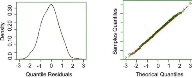
The adjustment of the binomial distribution with a logit link function for the selected variables can be seen in Figure 1. The “worm” graph in Figure 2 is a general diagnostic tool for residual analyses. The vertical axis represents the differences between theoretical and em-pirical distributions. The “worm” graph should be in the form of a cord, indicating a binomial data distribution in the present case in which consecutive points can be observed (Buuren and Fredricks, 2001). Figures 2 show that the worm graph of the binomial distribution with a logit link function is not adjusted very well.
The parameter estimates for the logistic regression and discrete choice model are shown in (Table 2).
The comparison of the estimates of the two meth-ods differs with respect to the intercept. However, when analyzing data of the behavior of the animals it is a little difficult to interpret the intercept in the logistic regres-sion model. Here the discrete choice model is proposed with one choice for the analyses of data from animals. With a discrete choice model for resource selection, the
i-th choice is described by the choice set of resource units (habitat or food) that are available to be chosen; and val-ues for variables that characterize all resource units in the choice set (e.g., vegetation type, elevation, etc.).
A comparison of models by the chi-squared test us-ing the logistic regression and discrete choice model pa-rameters is shown in (Table 3). This table shows the de-viance of DCM is -56.76 less than that of RL, and AIC of DCM is -58.76 less than that of RL.
Note that logistic regression has one degree of free-dom less than DCM since the latter does not have an intercept.
n o i s s e r g e R c i t s i g o
L DiscreteChoiceModel
s e l b a i r a
V Coefficient Std.err1 P-value2 Coefficients Std.err.
t n a t s n o
C -3.9758 1.2618 0.002 -
-2 c l c
a -0.3606 1.1461 0.753 -0.0747 1.2672
3 c l c
a -1.0449 1.4836 0.481 -1.1875 1.5949
4 c l c
a 0.4724 1.1233 0.674 0.7734 1.2807
d e _ l c
a 0.0127 0.0058 0.029 0.0176 0.0077
t n e c _ t g
h 0.0104 0.0049 0.034 0.0147 0.0064
t n e c _ p l
s -0.0171 0.0073 0.019 -0.0289 0.0103
Table 2 – Estimates of Logistic Regression and Discrete Choice Model parameters (DCM) for habitat selection of the spotted owl.
1Estimated standard errors output from the fitting process. 2The p-values shown are obtained by calculating the ratios of estimates to their standard errors and finding.
Figure 1 – Distribution of residual frequencies and QQ plot for Binomial distribution with logit link function.
Figure 2 – Worm graph of binomial distribution with logit link function.
samples that were taken separately of different unit types: available, used and non-used.
The similarity between the logistic regression and DCM graphs shown in (Figure 4) should be observed,
Table 3 – Comparison of models by the Q-squared test.
n o i s s e r g e R c i t s i g o
L DiscreteChoice
) M C D ( l e d o M e
c n a i v e
D 163.78 (383df) 107.02 (384df) C
I
A 177.78 119.02
Figure 5 – a. Slope position vs Log ( Discrete Choice Model (DCM ), b. Slope position vs Log (Logistic Regression).
Figure 6 – Log ( Discrete choice model (DCM)) vs Log ( Logistic Regression).
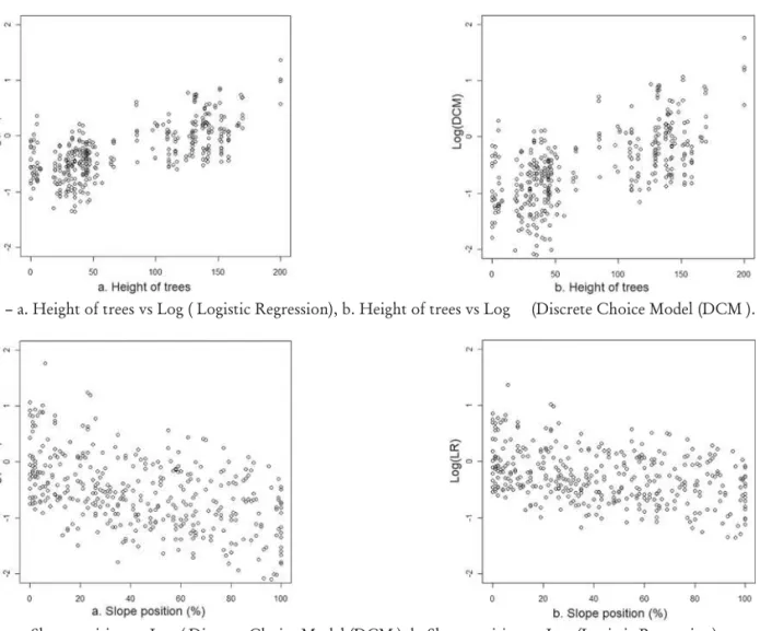
Figure 4 – a. Height of trees vs Log ( Logistic Regression), b. Height of trees vs Log (Discrete Choice Model (DCM ).
particularly the variable height of trees vs log (logistic regression) and the height of trees vs log (DCM) a light dispersion in the graph of the logistic regression.
In a same way it should be observed in Figure 5 (a) that the graph of the variable slope position vs log (Lo-gistic regression) and in Figure 5 (b) slope position vs log (DCM) a slight dispersion in the graph of the logis-tical regression.
In estimating each of the owl choices, it can be ob-served that the coefficients estimated for the logistic regression differ from the coefficients of all owl choices. The same occurred with DCM in estimates of choice model parameters for all owls. In the graph of the estimates of logistic regression and DCM there is a better adjustment with respect to DCM, and Table 3 indicates the best estimate of the deviance and Akaike information criteria (AIC) of the DCM model (Figure 6).
Conclusions
• Resource selection functions estimated by logistic re-gression successfully identified the resources critical to an animal population and predicted the occurrence of species in different locations.
model (DCM) were the best methods for predicting choices of the spotted owl.
• Parameter estimates for logistic regression and DCM with a one choice hadsimilar performances.
• An analysis made of all choices together differed from the analyses made choice by choice, justifying the use of random effect models for all animals considered si-multaneously. However, logistic regression and DCM can be generalized to include random effects.
References
Akaike, H. 1974. A new look at the statistical model identification. IEEE Transactions on Automatic Control 19: 716-723. Buuren, S.V; Fredricks, M. 2001. Worm plot: a simple diagnostic
device for modelling growth reference curves. Statistics in Medicine, 20: 1259-1277.
Fagen, R. 1988. Population effects of habitat change: a quantitative assessment. Journal of Wildlife Management 52: 41-46. FORTRAN 77. 1995. Programmer’s Guide. Wadsworth Pub. Co.,
Belmont, CA, USA.
Manski, C. 1988. Structural models for discrete data: the analysis of discrete choice. p.58-109. In: Leinhardt.S., ed. Sociological methodology. Jossey-Bass, San Francisco, CA,USA.
McCracken, M.L.; Manly, B.F.J.; Vander-Heyden, M. 1998. The use of discrete: choice models for evaluating resource selection. Journal of Agricultural, Biological, and Environmental Statistics 3: 268-279.
Manly, B.F.J.; McDdonald, L.L.; Thomas, D.L.; McDdonald, T.L.; Erickson, W.P. 2002. Resource Selection by Animals. 2ed. Kluwer Academic, London, UK.
McDonald, T.L.; Manly, B.F.J.; Nielson, R.M.; Diller, L.V. 2006. Discrete-choice modeling in wildlife studies exemplified by Northern Spotted Owl nighttime habitat
selection. Journal of Wildlife Management 70: 375-83.
MINITAB. 1997. Minitab User’s Guide 2: Data Analysis and Quality Tools. Minitab Inc., State College, PA, USA. The R Development Core Team, 2006. R: A Language and
Enviroment for Statistical Computing, Vienna, Austria. Available in http://www.R-project.org. [Accessed May 01, 2006]. Rosenzweig, M.L. 1981. A theory of habitat selection. Ecology 62:
327-335.
Ryan, N.; McDonald, T.L; Lamphear, D. 2004. Northern Spotted Owl Nighttime Site Selection Model. Report Western EcoSystems Technology,Cheyenne, WY, USA.
Train, K. 2003. Discrete Choice Methods with Simulation. University Press,Cambridge, UK.