Visegrad Four Countries – Case Study of
Econo-metric Panel Data Model for Regional
Competi-tiveness Evaluation
Nevima Jan
Abstract
The aim of the paper is to create an econometric panel data model with techniques using dummy
variables for simpliication of regional competitiveness evaluation in the case of selected EU
Visegrad Four (V4) countries. Theoretical background of the paper is based on the knowledge of theoretical concept and issues of regional competitiveness and productivity in the context of growth theories. The empirical part of the paper is focused on the application of linear panel data regression model for 35 regions at NUTS level 2 of selected V4 countries. The level of regional competitiveness is analysed by selected indicators evaluating the performance of the EU growth strategies objectives. Selection of explanatory variables in the panel data model
ap-propriately relects the level of competitive potential in NUTS 2 regions of the selected EU V4
countries in the reference period 2000 - 2008. The use of econometric panel data model seems to
be appropriate, since it marks the better capture of the dynamics of changes and ixed or random
effects that have occurred in the proposed explanatory variables. Based on the estimation of the
panel data model, econometric and economic veriication, the inal part of the paper includes a
comparison of results for all explanatory variables in NUTS 2 regions which are cross-sectional
and time used to determine the order of inluence of each NUTS 2 region of the selected V4
countries to the overall competitiveness of the European Union. The basic hypothesis assumes that the average value of EU 27 GDP per capita is considered as an ideal region, i.e., the most
competitive region. In the paper, we have observed contributions of each statistically signiicant
V4 NUTS 2 region to the average level of the whole EU 27 performance approximated by GDP per inhabitant in PPS. For the model purposes, the overall EU competitiveness is approximated with the average volume of GDP per capita in PPS for 271 NUTS 2 regions in the EU 27,
accord-ing to the NUTS 2008 -2011 classiication methodology.
Key words: competitiveness, Visegrad Four, NUTS 2 region, macro econometric modelling, panel data model
1. INTRODUCTION
Effectively analysed competitiveness means to be based on a deined concept of competitive -ness. For evaluation of regional competitiveness, we face the problem of the basic concept and
deinition of competitiveness due to absence of a consistent approach of its deinition. Com -petitiveness has become quite a common term used in many professional and non-specialized publications. Evaluation of the competitiveness issue is not less complicated. In the absence of mainstream views on the assessment of competitiveness, there is sample room for the presenta-tion of individual approaches to its evaluapresenta-tion. In our paper we will examine the possibility of evaluation the competitiveness of the regions of selected Czech and Slovak regions at NUTS 2 level in terms of analytic hierarchy process. The level of NUTS 2 regions for evaluation of
com-Vol. 4, Issue 4, pp. 3-15, December 2012
ISSN 1804-171X (Print), ISSN 1804-1728 (On-line), DOI: 10.7441/joc.2012.04.01
petitiveness seems to be legitimate especially because of the fact that European Commission ac-cents the level of regional units from aims of economic and social cohesion view and realization of structural aid in the EU member states. When making concept of suitable evaluation tools of
national and regional competitiveness it is necessary to suggest not only dificult but also simple
methods which enable quick evaluation of competitiveness by accessible tools. This paper ex-amines the possibility of evaluation the competitiveness of the regions of selected V4 countries at NUTS 2 level in terms of macro econometric modelling methodology (see e.g. Garrat, Lee, Pesaran, Shin, 2006; Šmídková, 1995) which as one of the techniques offers panel data regression
models (see e.g. Greene, 2007; Baltagi, 2008). Macro econometric modelling as a scientiic dis
-cipline allowing the estimation of the regression model, which would have suficient economic
importance to the appropriate regional indicators, which would be based on economic theories
and approaches directly, relect developments in the regions and their competitive potential.
2. THEORETICAL BASIS OF COMPETITIVENESS IN REGIONAL
CONTEXT
2.1 Definition of Competitiveness
The deinition of competitiveness is a problematic issue because of the lack of mainstream view for un-derstanding this term. Competitiveness remains a concept that is not well understood and that can be understood in different ways and levels despite widespread acceptance of its importance. Competitiveness is one of the fundamental criteria for evaluating economic performance, and
also relects the success in the broader comparison. The concept competitiveness is understood
at different levels especially at the microeconomic and the macroeconomic level, among which is the dif-ference. In original meaning the concept of competitiveness was applied only to companies and corporate strategies. Competitiveness of companies is usually understood as the ability to provide
products and services as well as or more effective than their main competitors (Porter, 2003).
Nowadays, competitiveness is one of the most monitored characteristic of national economies and is increasingly appearing in the evaluation of their prosperity, welfare and living standards.
The need for a theoretical deinition of competitiveness at the macroeconomic level, emerged
with the development of globalization process in world economy, so because of increased com-petition between countries. Despite of that, growth competitiveness of the territory belongs to the main priorities of the economic policies of the countries, there does not exist (compared
with the competitiveness at the microeconomic level) a uniform deinition and understanding
of national competitiveness. The concept of national or regional competitiveness is an object of numerous discussions. One of the most common interpretations of this term understood national
competitiveness as the ability to produce goods and services that are able to successfully face
inter-national competition, and people can enjoy growing and sustainable living standards (Klvačová, Malý, 2008). The Organization for Economic Cooperation and Development (OECD) deines
the national competitiveness as the degree or extent to which the country, in terms of open and fair trade, produce goods and services which meet the test of international markets while maintaining and increasing the real
incomes of its citizens in the long run (Garelli, 2002). Michael Porter suggests that the best way to
of living is determined by the productivity of its economy, which is measured by the value of its goods and services produced per unit of the nation’s human, capital and natural resources. True competitiveness, then, is measured by productivity. Productivity allows a nation to support high wages, a strong currency and attractive returns to capital
and with them a high standard of living” (Porter, 2003). The European Commission offers similar
deinition of this term in The Sixth Periodic Report on the Social and Economic Situation of
Regions in the EU: “...the ability to produce goods and services which meet the test of international markets, while at the same time maintaining high and sustainable levels of income or more generally, the ability of (regions)
to generate, while being exposed to external competition, relatively high income and employment levels”
(Euro-pean Commission, 1999). Euro(Euro-pean Commission presented in the Euro(Euro-pean Competitiveness Report that the economy is competitive if its population enjoy a high and constantly rising living standards and permanently high employment.
2.2 Concept of Regional Competitiveness
In last few years the topic about regional competitiveness stands in the front of economic interest. The concept of competitiveness has quickly spread into the regional level, but the notion of regional competitiveness is also contentious. Macroeconomic concept of national competitive-ness cannot be fully applied at the regional level because the regional competitivecompetitive-ness is much
worse and less clear deined; between these two concepts is a big difference (see e.g. Krugman,
1994). In the global economy regions are increasingly becoming the drivers of the economy and generally one of the most striking features of regional economies is the presence of clusters, or geographic concentrations of linked industries (Porter, 2003). Current economic fundamentals are threatened by the shifting of production activities to places with better conditions. The regional competitiveness is also affected by the regionalization of public policy because of the shifting of decision-making and coordination of activities at the regional level. Within govern-mental circles, interest has grown in the regional foundations of national competitiveness, and with developing new forms of regionally based policy interventions to help improve the competitive-ness of every region and major city, and hence the national economy as a whole. Regions play an increasingly important role in the economic development of states. Regional competitiveness can be understood as the result of joint efforts on the most productive use of internal resources development in the interac-tion with the use of external resources and development opportunities focused on sustainable increases in producinterac-tion
potential (Viturka, 2008).
The notion of regional competitiveness is also contentious. There are questions over how regions compete, and the extent to which regions are meaningful economic units to which the concept of competitiveness can be meaningfully applied. To talk of regional competitiveness would seem
to imply that regional economies are like irms or nation-states, and are in competition with one
another. However, regions are neither like irms nor nations. A region is not simply a scaled-up version
of the individual micro irm, nor the simple aggregation of many such irms. Regions are not eco
-nomic ‘actors’ in the sense that irms are. They have limited direct control of the activities that
take place within them, and they have a lower level of organizational identity and, arguably, unity
that irms and nation states. Rather, their economic prosperity can be signiicantly inluenced by the macro level iscal and monetary policies pursued by the nation-state.
worker, and employment. The latter are what might be termed ‘revealed’ measures of overall regional competitiveness, themselves the outcome of complex underlying factors and processes. Trends in a region’s aggregate performance, relative to trends in other regions, should reveal something about a region’s dynamic competitive advantage (Martin, 2005).
2.3 Approaches to Competitiveness Evaluation
Evaluation of competitiveness is no less complex as the deinition and understanding of the con -cept itself. Creation of competitiveness evaluation system in terms of the EU is greatly compli-cated by heterogeneity of countries and regions and also by own approach to the original concept of competitiveness. Evaluation of competitiveness in terms of differences between countries and regions should be measured through complex of economic (Enright et al, 1996), social and envi-ronmental criteria that can identify imbalance areas that cause main disparities. Currently not only quantitative but also qualitative development at the national level, and especially at the regional level, increase socio-economic attraction and create new opportunities that are fundamentals for subsequent overcoming disparities and increasing the competitiveness of the territory.
Competitiveness is most commonly evaluated by decomposition of aggregate macroeconomic indicators
of international organizations. Competitiveness of countries is monitored in many institutions; however, two well-known international institutes publish most reputable competitiveness re-ports. To compare a level of competitiveness of countries we can use the databases performed by
Institute for Management Development (IMD) and World Economic Forum (WEF). The World Economic
Forum publishes the Global Competitiveness Report (GCR) that produces annual competitiveness indices that rank national economies. Global Competitiveness Reports use two main aggregate indexes for measuring the level of competitiveness – the Global Competitiveness Index (GCI) and
the Business Competitiveness Index (BCI). The Institute for Management Development ranking on
competitiveness is realized in the World Competitiveness Yearbook (WCY) which provides a compre-hensive report on the competitiveness of countries assesses and analyses the national conditions for business competitiveness.
Regional competitiveness and its evaluation are issues constantly in the forefront of economic
scienc-es, which lacks a mainstream method of regional competitiveness monitoring and evaluation. Decomposition of aggregate macroeconomic indicators is most common used approach at the regional level, as well as comprehensive (mostly descriptive) analysis aimed at identifying the key
factors of regional development, productivity and economic growth (see e.g. Blažek, Viturka,
2008; Martin, 2003). Another approach is presented by EU structural indicators evaluation. These indicators are used for the assessment and the attainment of the objectives of the Lisbon
Strat-egy. We can also ind approach presented by application of analytic hierarchy process (Kiszová,
Nevima, 2012).
Finally, we can provide an approach of macro econometric modelling and create econometric regres-sion model (see e.g. Nevima, Melecký, 2012). Evaluation of regional competitiveness is determined by the chosen territorial region level, especially in terms of the European Union through the
Nomenclature of Units for Territorial Statistics (NUTS). No less importance is the reference period,
availability and periodicity of data, and selection of convenient speciic factors. For evaluation of
Comparing instruments for measuring and evaluation of competitiveness in terms of the EU is. There is linkages among instruments for measuring the EU competitiveness both national and regional level. There are different time period series at both levels, overlap of indicators of EU’s Growth Strategies at national and regional level. Further there is continuity between approach of the WEF and approach of the EU to measuring and evaluation of EU competitiveness. Between EU Competitiveness and cohesion policy there is a link in terms of Reports on Economic and Social Cohesion – 4th and 5th reports (2007, 2010) articulated a special indices for measuring and evaluation of competitiveness of European regions. Indicators and indices cover a broad area of economic, social and environmental interests, but coverage and reference period decrease in direct proportion to the lower territorial unit. Because of these clear and close link among
instruments (indicators and indices) for measuring of competitiveness is dificult to choose just
the “best approach” to evaluation.
3. RESEARCH METHODS USED
3.1 Methodological Background of the Analysis
Regional panel data models, they form a link between micro and macro components and are
con-structed mostly ad hoc. The explanatory and interpretive ability is mainly dependent on the
fulilment of the appropriate model and especially the available data and speciication of the
applied model.
Before the panel data model will be deined, let us have the beneits of this model compared to conventional linear regression models. In the panel data model, we can concentrate more than a simple classical regression model. We are better able to affect the dynamics of change, to which
the individual variables occurred. The main advantage is the detection of ixed, respectively
random effects, which we were able to diagnose only cross-application data or time series. An-other advantage is to design and test of complex models with an appropriate number of degrees of freedom. Further advantages and disadvantages of macro-econometric modelling states, for example Šmídková (1995). When using panel data model, there are also greatly eliminated varia-tions caused by aggregation of data sets used. Panel model is used not only for a mezzo-business applications, but also in areas such as microeconomics and macroeconomics (Heij, Ch. et al, 2004), it is suitable for the analysis of competitiveness.
3.2 Sample of Regions and Data Base for Econometric Analysis
The utilization of panel data model for empirical analysis of regional competitiveness in EU V4 countries was motivated by previous research of the authors. The partial research was con-centrated on application of panel data model in analysis and evaluation of competitiveness of 35 NUTS 2 Visegrad Four regions. For more detail of the results see Melecký, Nevima, (2011a, 2011b). The previous panel data model has been established on similar set of indicators and same reference period (2000-2008) in the frame of 35 NUTS 2 regions of Visegrad Countries. Paper wants to apply and test panel data model in different sample of observations presented by mac-roeconomic indicators of 35 selected NUTS 2 regions in V4 countries. The main selection criterion
found like a “mirror” of competitiveness performance in accordance with economic theory.
Data base econometric model for measuring regional competitiveness in 35 NUTS 2 regions of
V4 countries is made up of regional data, which was taken from the database of the European
Statistical Ofice - module Regional Statistics (Eurostat, 2011b) and from OECD Regional
Sta-tistics (OECD iLibrary, 2012). Under regional data has been used time series of four indicators
expressed in all volumes per inhabitant. We use annual basis regional data sheets that include: Gross domestic product (GDP), Gross ixed capital formation (GFCF), Gross expenditure on re-search and development (GERD) and Net disposable income of households (NDI). Comparabil-ity of data over time was ensured by using time series of the available indicators in PPS. Within each of selected indicators were always counted the average for the EU 27. The data analysis cover reference period 2000 - 2008.
3.3 The Specification of the Econometric Model of Panel Data for Selected V4
Regions
The estimate for each of the regions is the output of generally formulated model of the panel data. Due to it, we obtain the look at the level of competitiveness of each region. The access can be applied also on low number of observing in time, in our case for each NUTS 2 region during period 2000 – 2008 there were 9 observations. The negative of low number of observations in time is eliminated by using panel data and due to technique of dummy variables it is possible to
observe regional disparities (ixed effects). The logging for the estimate of panel linear regression
model with using of dummy variables for NUTS 2 regions of selected regions of Visegrad Four
countries is with using above speciied data base following (1):
(1)
Where:
GDPr,t Gross domestic product;
GFCFr,t Gross ixed capital formation;
GERDr,t Gross domestic expenditures on research and development;
NDIr,t Net disposable income;
α Constant;
β1,...,5 Slope parameter of regression model;
γr Differences parameter of ixed effects;
εr,t Random error;
Dr,t Binary variable for region speciication;
Dr,t = 1(if it takes data of the region “r” in time “t“; Dr,t = 0 otherwise;
r Indexes sectional characteristics (in our case NUTS 2 regions of V4; basic „region“ is average of EU 27 regions;
r = 1, 2,…, 35 (in our case 35 selected regions of V4);
t Indexes time; t = 2000, 2001,…, 2008.
W U W U U U W U W
U W
U W
U *)&) *(5' 1', '
*'3
Let’s introduce single input variables, which are included in the model. GDP is in the position of explained variable. GDP was chosen as it is one of the most important macroeconomic aggregate which is simultaneously suitable basic for competitiveness assessment of the country, but also for the regional level, where also NUTS 2 regions belong.
Paper comes from the OECD competitiveness deinition, according to which is competitiveness speciied by ability to produce products and services, which compete in the international competition test. At the same time it is able to keep or increase real GDP. Simultaneously, by keeping assigned hypothe-sis, it is valid, that GDP is the symptom of region competitiveness, as regions with increasing GDP have ideal presumption for long-term increasing of their competitiveness or otherwise. It is obviously
not always valid that with increasing level of GDP (i.e. increasing eficiency of regions) also the
rate of obtained competitiveness or competitive advantage grows. However, this presumption is initial for lots of grow theories and theories of regional competitiveness (see e.g. Martin, 2003;
Gardiner, Martin, Tyler, 2004; Hančlová et. al, 2010).
Explanatory variables of estimated model fulil the role of the source base for following growth
of GDP. Gross ixed capital formation (GFCF) due to international accounting is a basic part of
gross capital (capital investments), in which is also the change of inventories and net acquisition of valuables included. According to ESA 95 (European System of Accounts) methodology GFCF
consists of the net assets acquisition minus decrease of ixed assets at residential producers dur -ing the time period plus certain increas-ing towards the value of non-produced assets originated
as a consequence of production activity of producers or institutional units. Net ixed capital formation is the difference between gross ixed capital formation and ixed capital consumption.
It is estimated in purchase price including costs connected with instalment and other costs on transfer of the ownership. Fixed assets are tangible or intangible/invisible assets produced as the output from production process and are used in production process repeatedly or continuously during the one-year period. However, GFCF sense is much broader. It is an index of innovating
competitiveness which enables to increase production on modern technical base. Gross domestic
expenditures on research and development (GERD) are sources for further economic growth increasing as stimulation of basic and applied research creates big multiplication effects with
long-term eficiency and presumptions for long-term economic growth in economics. R&D is deined as creative work undertaken on a systematic basis in order to increase the stock of knowl -edge, including knowledge of man, culture and society and the use of this stock of knowledge to devise new applications. Net disposable income of households (NDI) is the result of current receipts and expenditures, primary and secondary disposal of incomes. It explicitly excludes
cap-ital transfers, real proits and loss from possession and consequences of the events as disasters. In contrast to gross disposable income it does not cover ixed capital consumption. Disposable income (gross or net) is the source of expenditures on inal consumption cover and savings in the sectors: governmental institutions, households and non-proit institutions for households. In sectors of non-inancial enterprises and inancial institutions is disposable income equal to
savings.
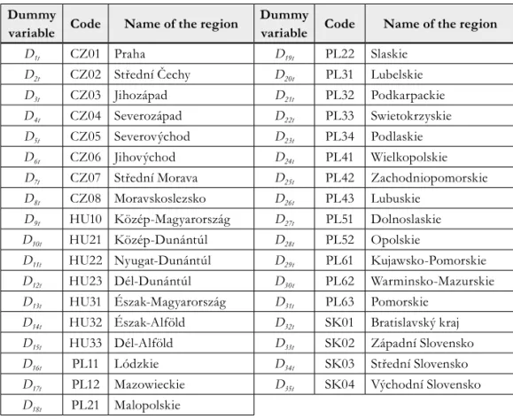
Tab. 1 – Assigning of the dummy variables for selected NUTS 2 Visegrad Four regions. Source: Eurostat, 2012, own elaboration
Dummy
variable Code Name of the region
Dummy
variable Code Name of the region
D1t CZ01 Praha D19t PL22 Slaskie
D2t CZ02 Střední Čechy D20t PL31 Lubelskie
D3t CZ03 Jihozápad D21t PL32 Podkarpackie
D4t CZ04 Severozápad D22t PL33 Swietokrzyskie
D5t CZ05 Severovýchod D23t PL34 Podlaskie
D6t CZ06 Jihovýchod D24t PL41 Wielkopolskie
D7t CZ07 Střední Morava D25t PL42 Zachodniopomorskie
D8t CZ08 Moravskoslezsko D26t PL43 Lubuskie
D9t HU10 Közép-Magyarország D27t PL51 Dolnoslaskie
D10t HU21 Közép-Dunántúl D28t PL52 Opolskie
D11t HU22 Nyugat-Dunántúl D29t PL61 Kujawsko-Pomorskie
D12t HU23 Dél-Dunántúl D30t PL62 Warminsko-Mazurskie
D13t HU31 Észak-Magyarország D31t PL63 Pomorskie
D14t HU32 Észak-Alföld D32t SK01 Bratislavský kraj
D15t HU33 Dél-Alföld D33t SK02 Západní Slovensko
D16t PL11 Lódzkie D34t SK03 Střední Slovensko
D17t PL12 Mazowieckie D35t SK04 Východní Slovensko
D18t PL21 Malopolskie
The model conception unambiguously determines which regions contribute to total average output of EU 27 by its economic level, which is approximated in endogenous variable by GDP per
capita. According to the hypothesis, that average of EU 27 stands for ideal region – the most
competi-tive region, it will be valid: the higher value of γr, the higher contribution of each NUTS 2 region to average level of economic output of whole EU 27. The regions with the highest contribution will be currently considered as the most competitive. This aspect is crucial for the model. The value of γr sets “distance” of V4 regions from level constant so called ideal region. Based on that contribution of regions towards total competitiveness is set. The process presents own access of the authors to the solved problems.
4. APPLICATION OF ECONOMETRIC PANEL DATA MODEL
4.1 The Estimate of Econometric Panel Data Model
The panel linear regression model will be estimated on method of least squares (OLS). The
sta-tistical veriication will be evaluated on 5 % level of statistic signiicance. For calculation SPSS
11 Economic veriication deals with the explanation of the meaning and formulating of the conclusions
on economic behaviour. The formula (2) is the result of (the irst) estimate of panel linear model
by dummy variables technique included all regions:
(2)
When we look at the formula, it is evident that all 3 explanatory variables have a different partial
in-luence on the development of average GDP per capita for EU 27. It is valid, at the same time, that
relations in formula (2) are inter-dependent, i.e. their signiicance, respectively their economic inluence can mutually overlap. Indicator of gross domestic expenditures on research and de
-velopment (GERD) has the highest partial inluence. The second partial inluence on economic
growth has increasing of net disposable income (NDI). The lowest impact has parameter of
gross ixed capital formation (GFCF).
After providing brief economic veriication, statistic and econometric veriication follows. The F–test
for evaluation of model signiicance as whole was used. At testing of model signiicance the model is statistically signiicant (level of signiicance 5 %). T-test for testing of partial
regres-sion coeficients was used. All of regresregres-sion coeficients (parameters) are statistically signiicant (lower than 5 % level of signiicance).
After statistical veriication view phase of econometric veriication follows. Econometric veriication
consists of testing of presence/absence of autocorrelation, heteroscedasticity and multicolinear-ity in the model. The autocorrelation was tested mathematically by Durbin – Watson (D–W) test and graphically by using autocorrelation (ACF) and partial autocorrelation (PACF) function. The value at D–W test at estimated model is 1.562. The value acts for evaluation of autocor-relation presence (serial dependency of residual components connected with sectional and time
inluences of panel model). According to critical values of D-W test, the presence of autocorrelation
was proved. It was acknowledged by orientation graphical test which veriies D-W test validity
(D-W test identiies autocorrelation of residues of the irst order). The test identiied presence of autocorrelation, especially of the irst order and conirmed also autocorrelation of higher orders.
However, this is not systematic. The fact led us to removing of autocorrelation of residues or to
reduction of their inluence.
In the view of this fact (presence of autocorrelation in model) we provide corrections of econo-metric model.
The correct estimate of the model was realised by Cochrane-Orcutt (C-O) method. C-O method is de facto algorithm for estimation of regression model by GLS method in case of
autocorrela-tion of irst order residues. It subsists in transformaautocorrela-tion of the original model when using Rho
parameter and its estimation by OLS method. In fact, correct estimation negated all above
pre-sented results of veriications. However, by C-O method application we removed autocorrelation of irst and higher orders from the model. The formula (3) shows the inal form of corrected estimation:
(3)
The estimate of formula signalizes that change of statistical signiicance of the model has not
occurred as whole and simultaneously all parameters of the corrected model are statistically
model was not proved. The value of D-W test is 1.949. It means that also according to critical
values of D-W statistics as well as according to orientation graphical test autocorrelation of irst
order was removed.
The next part of econometric veriication covers testing on heteroscedasticity and multicolin
-earity presence. The inal corrected model can be considered as homoscedastic on selected level of signiicance, which was veriied by graphical test. The graph could be constructed which
could evaluate development in each region. However, for purpose of the paper, the graph which evaluates development of standardised value of residua of corrected model against predicted value (GDP for all regions) was constructed. By evaluating the presence of multicolinearity in the model we have to consider eventuality of inner-cohesion of explanatory variables. For the
purpose of the work multicolinearity was orientation tested only by pair correlation coeficient.
The reasons of multicolinearity we can see mainly in economic view. There is a narrow structural
interconnection which is economic logical and justiiable. Another factor is a small number of
observations for each region. However, the value of pair correlation does not lower relevance of presented results. Moreover, due to methodical recommendation, multicolinearity is diagnosed
when it is statistically signiicant and the value of a pair correlation coeficient is about 0.9. In our case it is not so, as both conditions are not fulilled simultaneously.
4.2 Results Interpretation
After brief econometric veriication we can verify the model from economic point of view. When interpreting corrected estimate we have to emphasize that all 3 explanatory variables have different
partial inluence on development of average GDP per capita of EU 27. Simultaneously it is valid
that relations in the formula (3) are inter-dependent, i.e. their signiicance, respectively economic inluence can overlap and depends on explanatory variables selection. GERD has higher partial inluence, which was proved again (when increasing GERD by 1 million €, ceteris paribus condi -tion, the change of average level of expected GDP EU 27 can be increased about 10.412 millions
€). NDI has the second higher partial inluence on next economic growth, here by increasing by 1 million € the change of average level of expected GDP of EU 27 can be expected at approxi
-mately 1.898 million €, ceteris paribus. It was found out, that increasing of GFCF by 1 million can generate in average level of expected GDP of EU27 of 0.706 million € ceteris paribus, so GFCF has the lowest partial inluence.
It is necessary to emphasize that above interpreted results depend on partial contribution of 35 NUTS 2 regions of EU to overall EU 27 output in reference period 2000 – 2008. The dummy variables in the panel model show, which regions have the highest contribution to GDP formation of EU 27 in time and section of each NUTS 2 region. The complex results of econometric model
estimation in software SPSS 15.0 are introduced in appendix 1. The inal order of NUTS 2 re
-gions from their contribution view, respectively their inluence on EU 27 global competitiveness
measured by average level of GDP per capita is also given in appendix 1.
1 Prague. It means that created production by population is counted in Prague. In case of region PL121 we can identify problems with decreasing number of residents and leaving to work abroad because of local textile industry decline. We should remind that the above presented model does not present economic growth, but regional competitiveness. A model of economic growth on
contrary with a model of competitiveness has clearly deined form of input variables. Meanwhile
in this case we more or less search for suitable factors which contribute to growth of competi-tiveness due to GDP production. It is logical that by a choice of other explanatory variables we can expect different competitiveness order. As factors which determine its result level would change. To say it simply, meanwhile aggregate demand comes out of System of National Account by its four-sectors´ model; in case of competitiveness we have not had the “support” in the Sys-tem of National Account yet.
5. CONCLUSIONS
Presented linear regression model of panel data by using technique of dummy variables was based
on original concept of econometric model speciication. Average value of GDP per capita for EU
27 in period 2000 – 2008 is dependent variable at considering 3 independent variables (GFCF,
GERD, NDI) which were chosen arbitrary and also computed per capita. The basic hypothesis
assumes that average value of EU 27 GDP per capita is considered as an ideal region, it means the most competitive region. In the paper we have observed contributions of each statistically
sig-niicant V4 NUTS 2 regions to the average level of whole EU 27 performance approximated by
GDP per inhabitant in PPS. The regions with higher score of parameter γr have a positive impact to overall competitiveness of EU 27 because they contribute to average value of EU 27 GDP per inhabitant. The higher positive score of parameter γr , the higher positive impacts of NUTS 2 region on the overall competitiveness of EU 27. On the other hand, the regions with lower score of parameter γr have negative impacts to overall competitiveness of EU 27 because they reduce the average value of EU 27 GDP per inhabitant.
The paper outlined and veriied possible way for competitiveness analysis at regional level but
let’s simultaneously remind that above mentioned model is not model of economic growth, but
by contrast to model of competitiveness, it has explicitly deined form of input variables. Mean -while, in this case we partially look for suitable factors which contribute to competitiveness growth by means of GDP formation.
Acknowledgement
This paper was created in the students´ grant project “Seeking Factors and Barriers of the Competitiveness by Using of Selected Quantitative Methods”. Project registration number is SGS/1/2012.
References
Baltagi, B. H. (2008). Econometric analysis of panel data. New York: John Wiley & Sons Inc.
Blažek, L. & Viturka, M. et al. (2008). Analýza regionálních a mikroekonomických aspektů
konkurenceschopnosti. Brno: ESF MU, Centrum výzkumu konkurenční schopnosti.
Enright, M. J. et al (1996). The Challenge of Competitiveness. New York: St. Martin’s Press. 1.
2.
European Commission. (1999). Sixth Periodic Report on the Social and Economic Situation of
Regions in the EU. Retrieved September 20, 2011 from http://ec.europa.eu/regional_policy/
document/pdf/document/radi/en/pr6_complete_en.pdf.
Eurostat. (2011a). NUTS - Nomenclature of territorial units for statistics. Retrieved September 17, 2011 from http://epp.eurostat.ec.europa.eu/portal/page/portal/nuts_nomenclature/intro-duction.
Eurostat. (2011b). Regional Statistics. Retrieved September 20, 2011 from http://epp.eurostat. ec.europa.eu/portal/page/portal/statistics/search_database.
Garelli, S. (2002). Competitiveness of Nations: The Fundamentals. Retrieved September 20, 2011 from http://www.imd.ch/research/publications/wcy/index.cfm.
Garrat, A., Lee, K., Pesaran, M. H. & Shin, Y. (2006). Global and National Macroeconometric
Modelling. A long Run Structural Approach. Oxford: University Pres, Great Britain. http://
dx.doi.org/10.1093/0199296855.001.0001
Greene, W. H. (2007). Econometric analysis. New Jersey: Prentice Hall, Upper Sadle River.
Hančlová, J. et al. (2010). Makroekonometrické modelování české ekonomiky a vybraných ekonomik
EU. Ostrava: VŠB-TU Ostrava.
Heij, Ch. et al. (2004). Econometric Methods with Applications in Business and Economics. Oxford: Oxford University Press.
Klvačová, E. & Malý, J. (2008). Domnělé a skutečné bariéry konkurenceschopnosti EU a ČR. Praha: Vzdělávací středisko na podporu demokracie.
Kiszová, Z. & Nevima, J. Usage of analytic hierarchy process for evaluating of regional
competitiveness in case of the Czech Republic. In Proceedings of the 30th international conference
Mathematical methods in economics 2012. Karviná 11.-13.9.2012. Silesian University in Opava: School of Business Administration in Karviná.
Krugman, P. (1994). Competitiveness: A Dangerous Obsession. Foreign Affairs, 73(2), 28-44. http://dx.doi.org/10.2307/20045917
Martin, R. (2003). A Study on the Factors of Regional Competitiveness. A inal Report for the Euro
-pean Commission. Retrieved September 20, 2011 from http://ec.europa.eu/regional_policy/
sources/docgener/studies/pdf/3cr/competitiveness.pdf.
Martin, R. (2005). Thinking about Regional Competitiveness: Critical Issue. Retrieved September 17, 2011 from http://www.intelligenceeastmidlands.org.uk/uploads/documents/89137/ RonMartinpaper1.pdf.
Melecký, L. & Nevima, J. (2009). Ekonometrický přístup k hodnocení konkurenceschop
-nosti regionů v ČR. IMEA 2009. The 9th Annual Ph.D. Conference, 9 (1), 136-143.
Nevima, J. & Melecký, L. (2011a). Aplikace ekonometrického modelu panelových dat pro hodnocení regionální konkurenceschopnosti na příkladu zemí Visegrádské čtyřky. Auspicia, 8(1), 34-44.
Nevima, J. & Melecký, L. (2011b). Regional Competitiveness Evaluation of Visegrad Four
Countries through Econometric Panel Data Model. Liberec Economic Forum 2011. Proceedings of
the 10th International Conference, 10(1), 348-361.
4.
5.
6.
7.
8.
9. 10.
11.
12.
13.
14.
15.
16.
17.
18.
1 Nevima, J. & Kiszová, Z. Evaluation of regional competitiveness in case of the Czech and
Slovak Republic using analytic hierarchy process. In Proceedings of the 1st WSEAS International
Conference on Economics, Political and Law Science (EPLS ´12). Zlín, Česká republika: WSEAS
Press, 269-274
OECD Regional Statistics. (2012). OECD iLibrary. Retrieved July 19, 2012 from http:// www.oecd-ilibrary.org/urban-rural-and-regional-development/data/oecd-regional-statis-tics_region-data-en
Porter, M. E. (2003). The Economic Performance of Regions. Regional Studies, 37(6/7), 549-578.
Šmídková, K. (1995). Vývoj přístupů k makroekonometrickému modelování. Politická ekon-omie, 1, 113-124.
Contact information
Ing. Jan Nevima, Ph.D,
School of Business Administration in Karviná, Silesian University in Opava Department of Economics
Univerzitní náměstí 1934/3, 733 40 Karviná Tel: +420 728 854 443
E-mail: [email protected]
20.
21.
22.
23.