Numerical Simulations with the Galerkin Least Squares Finite Element
Method for the Burgers’ Equation on the Real Line
P.H.A. KONZEN1*, F.S. AZEVEDO2, E. SAUTER2 and P.R.A. ZINGANO2
Received on November 22, 2016 / Accepted on April 27, 2017
ABSTRACT.In this work we present an efficient Galerkin least squares finite element scheme to simu-late the Burgers’ equation on the whole real line and subjected to initial conditions with compact support. The numerical simulations are performed by considering a sequence of auxiliary spatially dimensionless Dirichlet’s problems parameterized by its numerical supportK˜. Gaining advantage from the well-known convective-diffusive effects of the Burgers’ equation, computations start by choosingK˜ so it contains the support of the initial condition and, as solution diffuses out,K˜ is increased appropriately. By direct compar-isons between numerical and analytic solutions and its asymptotic behavior, we conclude that the proposed scheme is accurate even for large times, and it can be applied to numerically investigate properties of this and similar equations on unbounded domains.
Keywords:Burgers’ equation on the real line, Galerkin least squares finite element method, asymptotic properties.
1 INTRODUCTION
Consider the viscous Burger’s equation defined on the real line:
∂u
∂t +bu
∂u
∂x =ν
∂2u
∂x2, (x∈R,t >0), (1.1) subjected to the initial condition:
u(x,0)=g(x), (x∈R), (1.2)
whereb=0 is a given parameter,ν >0 is a given viscosity coefficient andgis a given function with compact support onR.
*Corresponding author: Pedro Henrique de Almeida Konsen – E-mail: [email protected]
Burgers’ equation is known to have appeared firstly in 1915 in the work of Harry Bateman [10], but it receives its name after the Dutch physicist J.M. Burgers, who applied this equation in the understanding of turbulent fluids [12]. This homogeneous quasilinear parabolic partial differential equation appears in the modeling of several phenomena such as shock flows, wave propagation in combustion chambers, vehicular traffic movement, acoustic transmission, etc. (see, for instance, [21] and the references therein). Another import characteristic of this equation is its several well known analytic solutions in bounded and unbounded domains. Therefore, this equation is already a classical test case in mathematical analysis and numerical simulations of convective-diffusive partial differential equations.
From the analytic point of view the literature is rich in discussing solutions and properties for the Burgers’ equation on bounded and unbounded regions and subjected to a variety of initial and boundary conditions (see, for instance, [1, 9, 12, 20, 24, 28, 47, 52]). Now, from the numerical simulation point of view the majority of the studies found in the literature are concerned about the Burgers’ equation defined in a bounded region and subjected to Dirichlet’s boundary condi-tions. Several numerical schemes have been applied to simulate this problem, for instance: finite element methods [2, 3, 5, 14, 15, 16, 19, 22, 31, 35, 39, 40, 43, 45, 49, 55], finite difference methods [14, 22, 25, 38, 42], variational schemes [4, 13, 46], spectral methods [8, 37], Hardy’s multiquadric method [29], matched asymptotic expansion methods [44], multisymplectic box methods [51], homotopy analysis methods [32], the quintic B-spline collocation procedure [48], the gradient reproducing kernel particle method [27], quasi-interpolation techniques [54], uni-form Haar wavelets [33]. Numerical solutions by spatial discretization techniques of the Burg-ers’ equation in unbounded domains have been obtained by applying the artificial boundary method [26, 53, 50]. A comprehensive review of techniques for the solution of the Burgers’ equation is found in [57].
In this work we present an efficient numerical scheme based on the Galerkin least squares finite element method to simulate Burgers’ equation on the real line and subjected to initial conditions with compact support. The proposed scheme explore the convective-diffusive nature of the dif-ferential equation. If for small times the convective effects are predominant demanding very fine and localized meshes, for large times diffusion takes over and the solution tends to relax demand-ing less refined but large meshes. We deal with it by computdemand-ing the finite element discretization of a sequence of dimensionless spatially forms of the Burgers’ equation on a fixed mesh and parameterized by its domain. This idea has been proved very computational efficient producing accurate results.
In the works of Han [26] and Sun [50] the problem (1.1)-(1.2) has been faced applying artifi-cial boundary conditions to approximate it as a boundary-valued problem in a bounded domain, which they have solved by means of finite difference approximations. They have also tested their scheme comparing their computed solutions against analytic solutions for diffusion coefficients
In the next section we briefly discuss the analytic solution of problem (1.1)-(1.2) and its asymp-totic properties. In Section 3 we present the proposed time and space discretization of the spa-tially dimensionless form of the Burgers’ equation. In Section 4 we discuss the details of the implementation scheme. Then in Section 5 we present numerical experiments, which endorse the efficiency and accuracy of the scheme as to its potential to be applied to investigate solution properties in unbounded domains. Finally, in Section 6 we close by summarizing the principal aspects of this work.
2 ANALYTIC SOLUTION
Here we recall the well known closed-form expression foru(x,t)obtained by J. Cole and E. Hopf [17, 30]. Introducingβ(x,t)andβ0(x)by the Hopf-Cole transformation:
β(x,t):=exp
− b
2ν
x
0
u(y,t)d y
, β0(x):=exp
−b 2ν
x
0
g(y)d y
, (2.1)
one obtains thatβ solves the following initial value problem for the heat equation:
∂β ∂t =ν
∂2β
∂x2, (x ∈R,t>0) (2.2)
β(x,0)=β0(x), (x ∈R), (2.3)
whose unique bounded solution is given by Poisson’s formula:
β(x,t)= √1 4π νt
∞
−∞
e−|x−y|
2
4νt β0(y)d y, (x∈R,t >0). (2.4)
Sinceu= −2ν b
βx
β , it follows that:
u(x,t)= 1
b ∞
−∞
x−y
t e−
|x−y|2
4νt β0(y)d y
∞
−∞e−
|x−y|2
4νt β0(y)d y
, (x∈R,t >0). (2.5)
This also shows that problem (1.1)-(1.2) has a unique solutionu(·,t) ∈ C0
[0,∞),L1(R)
, given by (2.5) above, which satisfies:u∈C∞(R×(0,∞))andu(·,t)∈C0
(0,∞),Wk,p(R)
for everyk ≥1, p ≥1. Here,Wk,p(R)is the Sobolev space of functions inLp(R)whosek-th order derivatives belong to Lp(R). Moreover, by (2.5) and standard heat kernel estimates one gets that:
u(·,t)L2(R)=O(t− 1
4), u(·,t)L∞(
R)=O(t− 1
2), (2.6)
ux(·,t)L2(R)=O(t− 3
4), ux(·,t)
L∞(R)=O(t−1), (2.7)
ux x(·,t)L2(R)=O(t− 5
4), ux x(·,t)L∞(
R)=O(t− 3
2), (2.8)
A more refined analysis in [56] shows that the asymptotic limits:
γp:= lim t→∞t
1 2
1−1
p
u(·,t)Lp(R), 1≤ p≤ ∞, (2.9) are well defined and have the following values. Letmbe the solution mass, that is:
m= ∞
−∞
u(x,t)d x = ∞
−∞
u0(x)d x. (2.10)
For 1< p≤ ∞, we have:
γp= |
m| √
4π ν(4ν)
1 2p 2ν
bm
1−e−2mν FLp(R) (2.11) withF ∈ L1(R)∩L∞(R)defined by:
F(x)= e −x2
λ−herf(x), (2.12)
where erf(·)is the error function:
erf(x)= √2
π
x
0
e−ξ2dξ (2.13)
andλ,h are given by:
λ= 1+e
−bm2ν
2 , h=
1−e−bm2ν
2 . (2.14)
When p=1, the limit (2.9) is simply:
γ1= lim
t→∞u(·,t)L1(R)= |m|, (2.15)
and we further have:ux(·,t)L1(R)=O(t− 1
2),ux x(·,t)
L1(R)=O(t−1), and so on.
These results will be used in Section 5 as further evidence for the accuracy of the numerical approximation scheme developed in the next two sections.
3 FINITE ELEMENT SCHEME
We consider the following auxiliary Dirichlet’s problem:
∂u˜
∂t +
2b
(lb−la)˜
u∂u˜
∂x˜ = 4ν (lb−la)2
∂2u˜
∂x˜2, (x˜∈(−1,1),t>0), (3.1)
˜
u(x˜,0)= ˜g(x˜), (x˜ ∈(−1,1)), (3.2) ˜
u(−1,t)= ˜u(1,t)=0, (t >0), (3.3)
this space dimensionless problem and, for the sake of simplicity, we denote the domain length
lab:=lb−la, and we will omit the tilde, i.e., we will denotex˜simply byxandu˜byu.
Following the Rothe’s method, we start by discretizing equation (3.1) in time. To this end, we consider the followingθ-scheme for the time discretization of equation (3.1):
um+1−um
δt = − 2bθ
lab
um+1∂u
m+1
∂x −
2b(1−θ )
lab
um∂u
m
∂x
+ 4νθ lab2
∂2um+1
∂x2 +
4ν(1−θ )
l2ab
∂2um
∂x2
(3.4)
whereu0 =u(x,0),um denotes the approximation ofu(x,tm),m =1,2, . . .,tm =mδt,δt is a given time step size and 0≤ θ ≤1. For the sake of simplicity, from now on we denoteum+1
byu andumbyu0.
Now, we consider the following weak formulation of the problem defined by equations (3.4), (3.2) and (3.3): givenu0∈ H01(−1,1)findu∈ H01(−1,1)such that:
(ϕ,u)+2θ δt
lab
ϕ,bu∂u
∂x
+4θ δt lab2
∂ϕ
∂x, ν
∂u
∂x
−
ϕ,u0 +2(1−θ )δt lab
ϕ,bu0∂u 0
∂x
+4(1−θ )δt lab2
∂ϕ ∂x, ν
∂u0
∂x
=0
(3.5)
for allϕ∈ H01(−1,1). Here, and in the sequel,(·,·)denotes theL2(−1,1)inner product. Let us consider the following second order finite element triple(K,P2(K), ), where the cells K⊂Thare line segments forming a regular triangulationThof the segment[−1,1], the element shape functionsP2(K)= {v :K → R, v(x)=a0+a1x+a2x2,a0,a1,a2 ∈R}are second order polynomials, and the degrees of freedomare located at the end points of eachKand its middle point (see, for instance, [34, 41]). This allows us to define the finite element space:
Vh:= {v∈C0(−1,1):v|K∈ P2(K),∀K∈Th} ⊂H01(−1,1).
Then, following the Galerkin least squares method (see, for instance, [41]), we iteratively ap-proximate the solution of (3.1) subjected to (3.2) and (3.3) by the solution of the following full discrete problem: givenu0h ∈Vhfinduh∈ Vhsuch that:
(ϕi,uh)+ 2θ δt
lab
ϕi,buh
∂uh
∂x
+4θ δt l2ab
∂ϕ
i
∂x, ν
∂uh
∂x
+
θ δtsh(ϕi,uh)−
ϕi,u0h +
2(1−θ )δt
lab
ϕi,bu0h
∂u0h
∂x
+
4(1−θ )δt
l2ab
∂ϕi
∂x , ν
∂u0h
∂x
+(1−θ )δtsh(ϕi,u0h)=0
for allϕi,i =1,2, . . . ,N, in the basis of the finite element spaceVh. The Galerkin least square stabilization termshis given by:
sh(ϕ,u):=
T∈Th
δT
−4ν
l2ab
∂2ϕ ∂x2 +
2b lab
ϕ∂ϕ ∂x,−
4ν
lab2
∂2u
∂x2 + 2b lab
u∂u
∂x
, (3.7)
and the local stabilization parameterδT is chosen such that [11]:
δT =δ0lab0hT
4ν
lab0hT +
2buhL∞(−1,1)
−1
,
whereδ0is a small positive constant, andlab0 is the length of the initial reference domain (see next section for more details about the choice of the reference domain). We observe that using the fixedlab0 leads to a consistent formulation, sinceδT → 0 ashT → 0, but not otherwise, sincelab → ∞. Moreover, this choice has leaded us to a stable numerical scheme as we may observe from our numerical experiments (see Section 5).
At each time step, we solve the nonlinear system of equations (3.6) by the Newton’s method. The Newton’s formulation then reads: givenu0h ∈ Vh we iteratively compute approximations
unh+1ofuhby iterating:
J(u(n)h )δu(n)= −F(u(n)h ), (3.8a)
u(nh+1)=u(n)h +δu(n), (3.8b) whereF(unh)denotes the left-hand-side of equation (3.6) substituting thereuhbyunh,δunis the Newton update, and the Jacobian matrixJ(u)= [ᒇi,j]i,jN,N=0have its elements defined by:
ᒇi,j :=ϕi, ϕj+ 2θ δt
lab
ϕi,bϕj
∂u
∂x
+2θ δt lab
ϕi,bu
∂ϕj
∂x
+ 4θ δt lab2
∂ϕ
i
∂x, ν
∂ϕj
∂x
+θ δtsh′(ϕi,u;ϕj),
(3.9)
whereNcounts for the number of elements in the triangulation, and
s′h(ϕi,u;ϕj):= N−1
i=0
δTi
−4ν lab2
∂2ϕi
∂x2 + 2b lab
ϕi
∂ϕi
∂x,−
4ν
lab2
∂2ϕj
∂x2 + 2b lab
ϕj
∂u
∂x+
2b lab
u∂ϕj
∂x
. (3.10)
We now lead the discussion to the implementation of this Galerkin least squares finite element method (GLS-FEM) to simulate the Burgers’ equation defined on the whole real line and sub-jected to an initial condition with compact support.
4 IMPLEMENTATION SCHEME
tends to relax allowing the application of less refined meshes. By assuming an initial condition with compact support, numerical simulations of the auxiliary Dirichlet’s problem (3.1)-(3.3) may produce accurate solutions for finite times. To ensure the accuracy we just need to choose appro-priate time step and spatial mesh length, and pick the domain[la,lb]sufficiently large. However, the larger the physical time we would like to consider the larger[la,lb]should be.
The convective effects are predominant for small times and it is appropriate to work with a small [la,lb], which reduces the demanding on the number of vertices of the finite element mesh. On the other hand, as time increases, the solution spreads out demanding a larger[la,lb]but a less refined mesh. We deal with this paradigm as follows.
Let K := {x∈R: g(x)=0} ⊂ Rbe the compact support of the initial condition. Without loss of generality, we assume that 0 ∈ K and denote d = maxx∈K{|x|}. Also, let’s denote byKŴ the boundary elements of the finite element space(K, P2(K),). With this in mind, the implementation idea is to start simulating the auxiliary Dirichlet’s problem (3.1)-(3.3) by choosing an appropriate domain[la,lb] ⊃ K such thatlb−la >d (see Fig. 1). Then, at each time iterationm we check if the numerical support K˜m := {x ∈ : |umh(x)| > 10−15}is still a subset ofTh\ {KŴ}. If it is not the case, then we increase|la|and/or|lb|, interpolate the numerical solutionumh ontoTh, and we solve the next time step.
Figure 1: Illustration of the choice of the reference domain[la,lb].
We point out that the above implementation scheme does not demand one to rewrite the finite el-ement triangulation at each increasing of the reference domain[la,lb], since we always simulate using the same fixed triangulation built in the domain[−1,1].
As time increases and the solution diffuses out, it may be possible to increase the time stepδt gaining performance of the computations. This is particularly important for us, since we are also interested in investigating the accuracy of the proposed numerical scheme for large times. Therefore, we implemented a time step corrector based on an estimate of the rate of convergence of the Newton iterations. More precisely, at each time stepmwith step lengthδtm, we compute the convergence rate estimationρ = δun2/δu021/n, wheren is the number of Newton iterations required for convergence at this time stepm, and · 2denotes thel2vector norm (see [36] for more about this typical convergence rate estimation). We assume the convergence of the Newton iterations whenF(unh)2 <10−10. Then, ifρ > 0.1, we increaseδ
ρ < 0.05, we decrease it by the same percentage. To ensure a good precision, we allowed the time step corrector to take effect at most at each one-hundred time steps and we set 10−1as the larger time step allowed.
We summarize the implementation procedure as follows:
1. Set a uniform mesh withNvertices built in the domain[−1,1].
2. Set the finite element triangulationTh.
3. Set an appropriate[la,lb] ⊃K.
4. Set the initial solution vectoru0h ← [g(xi)]i2=N0+1, wherexiis the abscissa of thei-th degree of freedom.
5. Set the present solution vectoruh←u0h.
6. Set the time stepδt.
7. Loop over time steps:
(a) Loop over Newton steps:
i. Assemble the Newton system.
ii. Solve the system. iii. Setuh←uh+δuh. (b) IfK˜ ⊂Th\ {KŴ}, then:
i. Set to doublelaand/orlb.
ii. Interpolateuhconsidering the new reference domain.
(c) Correct time step.
(d) Setu0←u.
The numerical simulations were implemented in C++ using thedeal.IIopen source finite ele-ment library [6, 7]. We applied the UMFPACK sparse direct linear solver impleele-mented there to compute the Newton updateδum from equation (3.8a). Evaluation of the analytic solution, its asymptotic behavior and post processing procedures were performed with the help of the Python-based ecosystemScipy.
4.1 Computation of the analytic solution
For small values ofν this quadrature scheme was not able to accurately compute the analytical solution only by itself even setting hundreds of digits. However, we have satisfactorily overcome this issue (at least forν as small as 10−3) by observing that: (1) for x = y the integrand of the numerator in equation (2.5) is null; (2) the integrands have huge scale differences from the domain(−∞,x)to(x,∞); (3) the integrands exponentially tend to zero for|x−y| → ∞. These observations motivated us to rewrite those integrals as follows:
∞
−∞
I(x,y)d y=
N0−1
i=0 ai+1
ai
I(x,y)d y+
N1−1
j=0 bj+1
bj
I(x,y)d y,
where I(x,y) denote the integrands, ai = −L0 +ih0, h0 = (x +L0)/N0, x > −L0, i=0,1, . . . ,N0,bj =x+ j h1,h1=(L1−x)/N1,x<L1, j=0,1, . . . ,N1.
This implies that in order to evaluate the analytical solutionu at a given pointx, we computed 2(N0+N1)integrals using the already mentioned quadrature procedure. By choosing appropri-atelyL0,L1,N0andN1(which strongly depend onν), we could compute the analytical solution with at least 10 precision digits.
5 NUMERICAL EXPERIMENTS
Here we present some numerical experiments with the proposed GLS-FEM scheme applied to the Burgers’ equation on the real line. We first discuss the accuracy of the transient numerical solutions, and then explore their asymptotic behavior. Moreover, in Subsection 5.3 we finish our numerical experiments discussing an application to gas dynamic phenomenon.
5.1 Transient solutions
In the following we discuss the performance of the proposed numerical scheme for|b| =1 and for different diffusion parametersνat several timest. We assume the following initial condition:
u0(x)=
αe−10x2 ,−2≤x≤2,
0 ,otherwise ,
where we have chosenα≈0,89206, which give us an initial solution with compact support and massm= u0L1(R)=0.5. The transient numerical solutions presented here were obtained by setting the initial domain[la,lb] = [−2,2]and the initial time stepδt =10−4.
To investigate the accuracy of the computations we present the evolution of the global relative error of the computed numerical solutions, i.e.:
ǫ(t):= uh(·,t)−u(·,t)L2(R)
u(·,t)L2(R)
,
Firstly, let us shortly discuss about the choice of the parameters ofδ0(for the GLS-stabilization) andθ(for the time scheme). The later may be heuristically chosen as small as enough to stabilize the numerical computations. After extensive numerical experiments we concluded thatδ0=0.1 is an appropriate choice for 1 ≤ ν ≤ 10−4, which is corroborated with the following reported results.
The time scheme parameter θ is classically chosen as: (1)θ = 0 the explicit Euler method; (2)θ=0.5 the Crank-Nicolson method; (3)θ =1 the implicit Euler method. As our initial con-dition is very smooth, it is expected thatθ=0.5 should lead to a good numerical performance, i.e. a good balance between computational costs and precision. As an example, let us assume
b=1.0,ν=1, and compute the GLS-FEM solution attf =1000s usingN =400. Withθ=0 the proposed numerical scheme was unstable yielding to spurious solutions. Withθ=1 compu-tations needed 16375 time steps and 16421 overall Newton steps to yield a numeric solution with an overall relative errorǫ(tf) =2.72×10⁻¹. Now, withθ = 0.5 we need 16375 time steps, 16413 overall Newton steps, and reached a numeric solution withǫ(tf)=2.17×10⁻⁶.
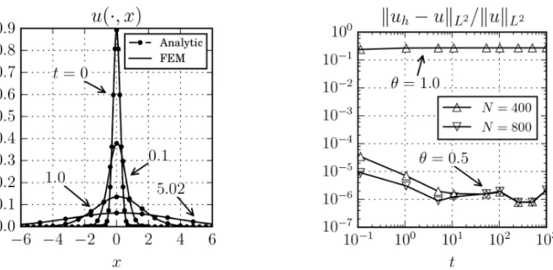
Figure 2: Transient numerical solutionsversusanalytic solutions forb =1 andν =1. Left: solution profiles att=0.0, 0.1, 1.0 and 5.02. Right: relative error on theL2-norm for numerical solutions with meshes ofN =400 and 800.
Figure 2 presents a comparison between GLS-FEM numerical solutions and analytic solutions computed at several times 0 ≤t ≤ 1000. The right graphic in Figure 2 presents the evolution of the global relative error of the computed numerical solutions. The figure showsǫyielded with
θ =1.0 and N =400, and also withθ =0.5 and N =400, 800. It is clear that the choice of
θ =0.5 has produced more accurate results withǫ(t) < 10−4for both meshes. From now on, we will assumeθ =0.5.
solutions withN =400. For the chosen parameters the Burgers’ equation is diffusion dominated (P´eclet numberPe<1), and we can observe that the solution rapidly diffuses out.
Now, Figure 3 presents the results found whenb= −1 andν=0.1. In this case, the convective effects are stronger, but the solution is still strongly diffusive, as we can observe by the solution profiles given on the left graphic of this figure. The numerical solution has again a good accuracy as one can see at the right graphic of this figure. Moreover, we point out that for small timest
the numerical scheme has a truncation error of at least the orderh2. However, for large times the diffusion effects are much stronger and, together with the increasing of the time step, causes the lost of such truncation order.
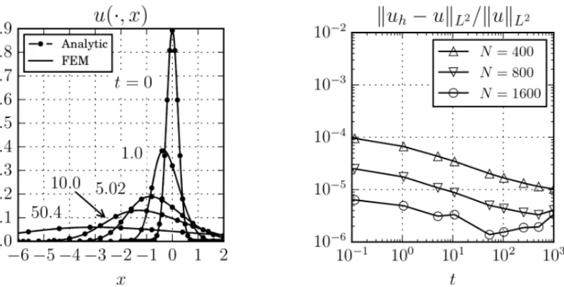
Figure 3: Transient numerical solutionsversus analytic solutions forb = −1 and ν = 10−1. Left: numerical solution withN =400 and analytic solution profiles att =0.0, 1.0, 5.02, 10.0 and 50.4. Right: relative error on theL2-norm for numerical solutions with meshes ofN =400, 800 and 1600.
As we decrease the diffusion coefficient we need more refined meshes to obtain such accurate results. The Figure 4 shows the comparison between numerical and analytic solution for the case ofb = 1 and ν = 10−2. Here, the convection effects are much stronger for small times and even a mesh withN = 1600 was not enough to ensure a relative error of 10−4. Nevertheless, the results presented in this figure indicate that further refinements will produce such accurate numerical results. We will come back to this point later.
Figure 4: Transient numerical solutionsversusanalytic solutions forb=1 andν =10−2. Left: numerical solution withN =400 and analytic solution profiles att =0.0, 1.0, 5.02, 10.0 and 50.4. Right: relative error on theL2-norm for numerical solutions with meshes ofN =400, 800 and 1600.
Since it is very computationally demanding to compute the analytic solution for smaller values of the diffusion parameter, we are not further able to globally compare the numerical and ana-lytic solution by accurately evaluating the relative errorǫ. However, we may still investigate the accuracy of the numerical scheme by analyzing its asymptotic behavior.
5.2 Asymptotic behavior
As a further evidence of the accuracy of the proposed numerical scheme, we compare the asymp-totic behavior of the numerical and analytic solutions by evaluating theγplimits defined in equa-tions (2.9), (2.11), and (2.15). This is done by computing what we call the numericalγp, which we define as:
˜
γp:=t 1 2
1−1p
f uh(·,tf)Lp(R), (5.1) wheretf is such thatF(uh(·,tf))2<10−9, i.e, thel2vector norm of the residual att =tf is less or equal to 10−9. We note that this provides an approximation ofγpas the numerical solution
uh approximates the analytic solutionu, andtf is large enough. Moreover we observe that this is a very fine test of the accuracy of the numerical solution, since it allowed us to check it for very large times.
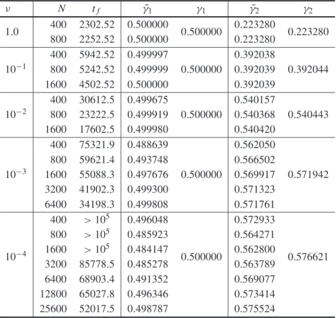
In Table 1 we present the computed values ofγ˜pversusγp for p = 1 (mass) and for p = 2 for solutions with diffusion coefficients from 1 to 10−4. The numerical scheme parameters were chosen as in the last subsection.
In opposition to the analytic solution given by equation (2.5), we observe thatγpcan be easily computed also for very small diffusive parameters. This allows us to globally measure the ac-curacy of the numerical solution even for high convective regimes. Going back to Table 1, the comparison betweenγ˜1andγ1corroborates that the numerical scheme is not mass conserving, but the mass loss can be kept low by using a sufficiently refined mesh.
Finally we note thatγ˜2also under-determines γ2. This is a qualitative indication of the good behavior of the numerical solution for large times, sincet1/4u(·,t)L2(R) is a monotonic in-creasing function for large times.
5.3 An application to gas dynamic phenomena
We finish our numerical experiments with an application to gas dynamic phenomenon. The convection and decay of a compression pulse of an isentropic gas can be modeled by the Burgers’ equation (1.1) with a Dirac delta function at zero time (see [23], Section 7.2). Defining a Reynolds number by Re:=m/(2ν), we have the following analytic solution
u(x,t)=
2ν
t
e−0.5n2 P+IC
, (t>0), (5.2)
wheren=x/(2νt)1/2,
P = √
2π
eRe−1, IC = ∞
n
Table 1: Numericalγ˜pversusanalyticγpforp=1 andp=2.
ν N tf γ˜1 γ1 γ˜2 γ2
1.0 400 2302.52 0.500000 0.500000 0.223280 0.223280 800 2252.52 0.500000 0.223280
10−1
400 5942.52 0.499997
0.500000
0.392038
0.392044 800 5242.52 0.499999 0.392039
1600 4502.52 0.500000 0.392039
10−2
400 30612.5 0.499675
0.500000
0.540157
0.540443 800 23222.5 0.499919 0.540368
1600 17602.5 0.499980 0.540420
10−3
400 75321.9 0.488639
0.500000
0.562050
0.571942 800 59621.4 0.493748 0.566502
1600 55088.3 0.497676 0.569917 3200 41902.3 0.499300 0.571323 6400 34198.3 0.499808 0.571761
10−4
400 >105 0.496048
0.500000
0.572933
0.576621 800 >105 0.485923 0.564271
1600 >105 0.484147 0.562800 3200 85778.5 0.485278 0.563789 6400 68903.4 0.491352 0.569077 12800 65027.8 0.496346 0.573414 25600 52017.5 0.498787 0.575524
The proposed GSL-FEM scheme can be applied to simulate this physical problem, for instance, by simulating (1.1)-(1.2) with
g(x)= m σ√2πe
−0.5(x/σ )2, (x
∈R), (5.3)
where we have changed the Dirac function atx=0 by a Gaussian function of massm.
Figure 6 shows the analytic solution (5.2) and the GLS-FEM numerical solution of problem (1.1)-(1.2) with the above g(x)at t = tf for several values of Re. In all cases we have set
m=1.0,σ =0.01,N =1600, andtf as defined in the last subsection. Again we observe a very good agreement between numerical and analytic solutions for very large times, even that here the initial solution has been grossly approximated. The effect of such approximation is however more notable for small times, which indicates a time delay in the numerical solutions.
6 FINAL CONSIDERATIONS
Figure 6: Analytic solution (5.2) and GLS-FEM solution for the convection and decay of a compression pulse. Re=3: solution computed at tf = 5704s. Re = 30: tf = 24838s. Re=90:tf =40987s.
compact support. The scheme consists in computing the finite element discretization of a se-quence of dimensionless spatially forms of the Burgers’ equation on a fixed triangulation and parameterized by its domain, which is chosen to contain the numerical support of the solution at each time step.
In order to investigate the accuracy of the proposed scheme, we performed direct comparisons between numerical and analytic solutions. For moderated diffusion coefficients the comparisons showed the scheme can be very accurate if one works with sufficiently refined meshes. Moreover, by analyzing asymptotic parameters of the solutions we could argue that the scheme is accurate even for very large times.
As we may expect the scheme demands more and more refined meshes as we decrease the dif-fusion parameter. An alternative would be to work with automatic local refined meshes. We observe that this could be particularly tricky, because one will need to be careful at each time that the reference domain is enlarged.
Finally we recall the Burgers’ equation is a prototype for many scientific related problems, and the proposed numerical scheme can be extended as well to assist the study of such related problems. For instance, it can be used to provide insights into analytic studies of problems on the whole real line.
RESUMO. Neste trabalho, apresentamos um eficiente esquema de elementos finitos com m´ınimos quadrados de Galerkin para simular a equac¸˜ao de Burgers na reta toda, sujeita a condic¸˜oes iniciais com suporte compacto. As simulac¸˜oes num´ericas foram realizadas
parametrizada pelo seu suporte num´ericoK. Tomando vantagem dos bem conhecidos efeitos˜ convectivos e difusivos da equac¸˜ao de Burgers, as computac¸˜oes iniciam-se escolhendoK˜
de forma a conter o suporte da condic¸˜ao inicial e, conforme a soluc¸˜ao se difunde,K˜ ´e au-mentada apropriadamente. Por comparac¸˜ao direta entre as soluc¸˜oes anal´ıtica e num´erica e,
pelo seus comportamentos assint´oticos, conclu´ımos que o esquema proposto ´e preciso mesmo para tempos grandes. Assim, este pode ser aplicado para numericamente investigar
proprie-dades desta e de similares equac¸˜oes em dom´ınios n˜ao limitados.
Palavras-chave: equac¸˜ao de Burgers na reta, m´etodo de elementos finitos com m´ınimos
quadrados de Galerkin, propriedades assint´oticas.
REFERENCES
[1] M.B. Abd el Malek & S.M.A. El-Mansi. Group theoretic methods applied to Burgers’ equation.J. Comput. Appl. Math.,115(2000), 1–12.
[2] E.N. Aksan. A numerical solution of Burgers’ equation by finite element method constructed on the method of discretization in time.Appl. Math. Comput.,170(2005), 895–904.
[3] E.N. Aksan. Quadratic B-spline finite element method for numerical solution of the Burgers’ equa-tion.Appl. Math. Comput.,174(2006), 884–896.
[4] E.N. Aksan & A. ¨Ozdecs. A numerical solution of Burgers’ equation. Appl. Math. Comput.,
156(2004), 395–402.
[5] P. Arminjon & C. Beauchamp. Continuous and discontinuous finite element methods for Burgers’ equation.Comput. Methods Appl. Mech. Engrg.,25(1981), 65–84.
[6] W. Bangerth, D. Davydov, T. Heister, L. Heltai, G. Kanschat, M. Kronbichler, M. Maier, B. Turcksin & D. Wells. Thedeal.IIlibrary, version 8.47.Journal of Numerical Mathematics,24(2016).
[7] W. Bangerth, R. Hartmann & G. Kanschat. deal.II – a general purpose object oriented finite element library.ACM Trans. Math. Softw.,33(4)(2007), 24/1–24/27.
[8] C. Basdevant, M. Deville, P. Haldenwang, J.M. Lacroix, J. Quazzani, R. Peyret & P. Orlandi. Spectral and finite difference solutions of the Burgers’ equation.Comput Fluids,14(1986), 23–41.
[9] M. Basto, V. Semiao & F. Calheiros. Dynamics in spectral solutions of Burgers equation.J. Comput. Appl. Math.,205(2006), 296–304.
[10] M.A.H. Bateman. Some recent researches on the motion of fluids.Mon. Wea. Rev., 43 (1915), 163–170.
[11] M. Braack. Finite elemente. available online,http://www.numerik.uni-kiel.de/˜mabr/ lehre/skripte/fem-braack.pdf, Jan. 2015.
[12] J.M. Burgers.The nonlinear diffusion equation. Springer, (1974).
[13] J. Caldwell, R. Saunders & P. Wanless. A note on variation-iterative schemes applied to Burgers’ equation.J. Comput. Phys.,58(1985), 275–281.
[14] J. Caldwell & P. Smith. Solution of Burgers’ equation with a large Reynolds number.Appl. Math. Modelling,6(1982), 381–385.
[16] J. Caldwell, P. Wanless & A.E. Cook. Solution of Burgers’ equation for large Reynolds number using finite elements with moving nodes.Appl. Math. Modelling,11(1987), 211–214.
[17] J.D. Cole. On a quasi-linear parabolic equation occurring in aerodynamics.Quart. Appl. Math,
9(3) (1951), 225–236.
[18] R. Courant & K.O. Friedrichs. Supersonic flow and shock waves. Springer, New York, (1948).
[19] A. Dogan. A Galerkin finite element method to Burgers’ equation.Appl. Math. Comput.,157(2004), 331–346.
[20] L.C. Evans.Partial differential equations, volume 19 ofGraduate Studies in Mathematics. The American Mathematical Society, 2nd edition, (2010).
[21] C.A. Fletcher.Numerical Solutions of Partial Differential Equations, chapter Burgers’ equation: a model for all reasons, pages 139–225. Nort-Holland, Amsterdam, (1982).
[22] C.A. Fletcher. A comparison of finite element and finite difference solutions of the one- and two-dimensional Burgers’ equations.J. Comput. Phys.,51(1983), 159–188.
[23] C.A. Fletcher. The Galerkin method and Burgers’ equation. In: Computational techniques for differ-ential equations. Mathematics Studies 83. Ed.: J. Noye, North-Holland, (1984).
[24] A. Gorguis. A comparision between Cole-Hopf transformation and the decomposition method for solving Burgers’ equations.Appl. Math. Comput.,173(2006), 126–136.
[25] M. G¨ulsu. A finite difference approach for solution of Burgers’ equation.Appl. Math. Comput.,
175(2006), 1245–1255.
[26] H.-d. Han, X.-n. Wu & Z.-l. Xu. Artificial boundary method for Burgers’ equation using nonlinear boundary conditions.J. Comput. Math.,24(3) (2006), 295–304.
[27] A. Hashemian & H. Shodja. A meshless approach for solution of Burgers’ equation.J. Comput. Appl. Math.,220(2008), 226–239.
[28] C.J. Holland. On the limiting behavior of Burger’s equation.J. Math. Anal. Appl.,57(1977), 156–160.
[29] Y.C. Hon & X.Z. Mao. An efficient numerical scheme for Burgers’ equation.J. Comput. Appl. Math.,
95(1998), 37–50.
[30] E. Hopf. The partial differential equationut+uux=µux x.Comm. Pure and Appl. Math.,3(1950),
201–230.
[31] A.N. Hrymak, G.J. McRae & A.W. Westerberg. An implementation of a moving finite element method.J. Comput. Phys.,63(1986), 168–190.
[32] M. Inc. On numerical solution of Burgers’ equation by homotopy analysis method.J. Phys. A,
372(2008), 356–360.
[33] R. Jiwari. A hybrid numerical scheme for the numerical solution of the Burgers’ equation.Comput. Phys. Commun.,188(2015), 59–67.
[34] C. Johnson.Numerical solutions of partial differential equations by the finite element method. Dover, (2009).
[35] M. Kadalbajoo & A. Awasthi. A numerical method based on Crank-Nicolson scheme for Burgers’ equation.Appl. Math. Comput.,182(2006), 1430–1442.
[36] C.T. Kelley.Solving nonlinear equations with the Newton’s method. SIAM, (2003).
[38] S. Kutluay, A.R. Bahadir & A. ¨Ozdes¸. Numerical solution of one-dimensional Burgers equation: explicit and exact-explicit finite difference methods.J. Comput. Appl. Math.,103(1999), 251–261.
[39] S. Kutluay, A. Esen & I. Dag. Numerical solutions of the Burgers’ equation by the least-squares quadratic B-spline finite element method.J. Comput. Appl. Math.,167(2004), 21–33.
[40] C.A. Ladeia, N.M. Romero, P.L. Natti & E.R. Cirilo. Formulac¸˜oes semi-discretas para a equac¸˜ao 1d de Burgers.TEMA (S˜ao Carlos),14(3)(2013), 319–331.
[41] Mats G. Larson & Fredrik Bengzon.The Finite Element Method: Theory, Implementation, and Ap-plications. Springer-Verlag Berlin Heidelberg, (2013).
[42] V. Mukundan & A. Awasthi. Efficient numerical techniques for Burgers’ equation.Appl. Math. Com-put.,262(2015), 282–297.
[43] T. ¨Ozis¸, E.N. Aksan & A. ¨Ozdes¸. A finite element approach for solution of Burgers’ equation.Appl. Math. Comput.,139(2003), 417–428.
[44] T. ¨Ozis¸ & Y. Aslan. The semi-approximate approach for solving Burgers’ equation with high Reynolds number.Appl. Math. Comput.,163(2005), 131–145.
[45] T. ¨Ozis¸, A. Esen & S. Kutluay. Numerical solution of Burgers’ equation by quadratic B-spline finite elements.Appl. Math. Comput.,165(2005), 237–249.
[46] T. Ozis & A. Ozdes. A direct variational methods applied to Burgers’ equation.J. Comput. Appl. Math.,71(1996), 163–175.
[47] E.Y. Rodin. On some approximate and exact solutions of boundary value problems for Burgers’ equa-tion.J. Math. Anal. Appl.,30(1970), 401–414.
[48] B. Saka & ˙I. Da ˘g. A numerical study of the Burgers’ equation.J. Frankl. Inst.,345(2008), 328–348.
[49] L. Shao, X. Feng & Y. He. The local discontinuous Galerkin finite element method for Burgers’ equation.Math. Comput. Model.,54(2011), 2943–2954.
[50] Z.-Z. Sun & X.-N. Wu. A difference scheme for Burgers equation in an unbounded domain.Appl. Math. Comput.,209(2009), 285–304.
[51] A.H.A.E. Tabatabaei, E. Shakour & M. Dehghan. Some implicit methods for the numerical solution of Burgers’ equation.Appl. Math. Comput.,191(2007), 560–570.
[52] W.L. Wood. An exact solution for Burger’s equation.Commun. Numer. Meth. Engng.,22(2006), 797–798.
[53] X. Wu & J. Zhang. Artificial boundary method for two-dimensional Burgers’ equation.Comput. Math. Appl.,56(2008), 242–256.
[54] M. Xu, R.-H. Wang, J.-H. Zhang & Q. Fang. A novel numerical scheme for solving Burgers’ equation. Appl. Math. Comput.,217(2011), 4473–4482.
[55] X.H. Zhang, J. Ouyang & L. Zhang. Element-free characteristic Galerkin method for Burgers’ equa-tion.Eng. Anal. Boundary Elem.,33(2009), 356–362.
[56] P.R. Zingano. Some asymptotic limits for solutions of Burgers equation. available at: http:// arxiv.org/pdf/math/0512503.pdf, 1997. Universidade Federal do Rio Grande do Sul.
![Figure 1: Illustration of the choice of the reference domain [ l a , l b ] .](https://thumb-eu.123doks.com/thumbv2/123dok_br/18983904.458106/7.1063.265.864.685.942/figure-illustration-choice-reference-domain-l-l-b.webp)