Dissipative Non-linear Schrodinger equation with variable coefficient in a stenosed elastic tube filled with a viscous fluid
Kim Gaik Taya,Yaan Yee Choyb,Chee Tiong Ongc and Hilmi Demirayd
a
Universiti Tun Hussein Onn Malaysia, Faculty of Science, Art and Heritage, Department of Science and Mathematics, 86400 Parit Raja, Batu Pahat, Johor, Malaysia.
b ,c
Universiti Teknologi Malaysia, Faculty of Science, Department of Mathematics, 81310 Skudai, Johor, Malaysia.
d
Isik University, Faculty of Arts and Sciences, Department of Mathematics, B¨uy¨ukdere Caddesi, 34398, Maslak-Istanbul-Turkey.
Abstract
In the present work, by considering the artery as a prestressed thin-walled elastic tube with a symmetrical stenosis and the blood as an incompressible viscous fluid, we have studied the amplitude modulation of nonlinear waves in such a composite medium through the use of the reductive perturbation method [23]. The governing evolutions can be reduced to the dissipative non-linear Schrodinger (NLS) equation with variable coefficient. The progressive wave solution to the above non-linear evolution equation is then sought.
Keywords: Elastic tube with stenosis, viscous fluid, nonlinear Schrodinger equation. 1. Introduction
Due to its applications in arterial mechanics, the propagation of pressure pulses in fluid-filled distensible tubes has been studied by several researchers (Pedley [1] and Fung [2]). As far as the biological applications are concerned, most of the works on wave propagation in compliant tubes have considered small amplitude waves ignoring the nonlinear effects and focused on the dispersive character of waves (see, Atabek and Lew [3], Rachev [4] and Demiray [5]). However, when the nonlinear terms arising from the constitutive equations and kinematical relations are introduced, one has to consider either finite amplitude, or small-but-finite amplitude waves, depending on the order of nonlinearity.
Rudinger [6], Ling and Atabek [7], Anliker et al [8] and Tait and Moodie [9] observed the propagation of finite amplitude waves in fluid-filled elastic or viscoelastic tube by using the characteristics method to study the formation of shock. On the other hand, the propagation of small-but-finite amplitude waves in distensible tubes has been investigated by Johnson [10], Hashizume [11], and Yomosa [12] by employing various asymptotic methods.
Later, in a series of works of Demiray and Antar [13]-[15], they treated the artery as an incompressible, prestressed, thin and isotropic elastic tube and the blood as an incompress-ible inviscid, viscous or layered fluid. Then, by using the reductive perturbation method in the long-wave approximation, they obtained KdV, Burgers’ and KdV-Burgers’ type equations, respectively.
Recently, Tay and co-workers [16]-[18] studied the non-linear waves propagation in a pre-stressed thin elastic tube with a symmetrical stenonis filled with inviscid, viscous and Newtonian fluid with variable viscosity, they showed that the governing equations can be reduced to forced Kortewed-de Vries, forced perturbed Kortewed-de Vries and forced Kortewed-de Vries-Burgers equations, respectively.
The modulation of small-but-finite amplitude pressure waves in a fluid-filled distensible, lin-ear elastic tube has been examined by Ravindran and Prasad [19]. They obtained the non-linlin-ear Schrodinger (NLS) equation equation. The work of of non-linear waves modulation in a pre-stressed thin elastic tube filled with inviscid or viscous fluid has been carried out by Demiray and co-worker [20]-[22]. They showed that the governing equations can be reduced to NLS and dissipative NLS equations, respectively. The NLS equation is the simplest representative
tion describing the self-modulation of one-dimensional monochromatic plane waves in dispersive media. It has a balance between the nonlinearity and dispersion.
In the present work, considering the artery as an incompressible, prestressed, thin-walled elastic tube with a symmetrical stenosis and the blood as an averaged viscous fluid, we have studied the amplitude modulation of non-linear waves in such a composite medium by using the reductive perturbation method [23]. We obtained the dissipative NLS equation with variable coefficient. We then sought the progressive wave solution to the non-linear evolution equation obtained.
2. Basic equations and theoretical preliminaries
In this section, we shall give the derivation of the field equations of an elastic tube, which is considered to be a model for an artery, and a viscous fluid, which is assumed to be a model for blood.
2.1 Equations of tube
In this sub-section, we shall derive the governing equations of an elastic tube filled with a viscous fluid. Such a combination of a solid and a fluid is considered to be a model for blood flow in arteries.
For a healthy human being, the systolic pressure is about 120 mm Hg, and the diastolic pressure is around 80 mm Hg. This means that the arteries are subjected to a mean pressure P0 = 100 mm Hg, and in the course of blood flow, a dynamical pressure increment ΔP = ± 20 mm Hg is added on this initial field. Moreover, experimental studies (Fung [2]) revealed that the arteries are also subjected to an initial axial stretch λz, which is about λz = 1.6. These observations show that the arteries are initially subjected to static deformation both in the radial and the axial directions, and a dynamical pressure (or a radial displacement u∗ ) is
superimposed on this initial deformation. Due to the external tethering in the axial direction, the effect of axial displacement is neglected.
Now, we consider a thin and long tube of circular cross-section with initial reference radius R0 in the cylindrical polar coordinates (R∗,Θ, Z∗). Then, the position vector of a point on the tube can be described by
R = R0er+Z∗ez, (1)
whereer,eθ and ez are the unit base vectors in the cylindrical polar coordinates andZ∗ is the
axial coordinates of a material point in the natural state.
The arc lengths along the meridional and circumferential curves are given by
dSZ =dZ∗, dSΘ=R0dΘ. (2)
Motivated with the experimental observations (Fung [2]), we shall assume that the elas-tic tube is subjected to an axial stretch ratio λz, and the static pressure P0∗(Z∗). Then, the deformation may be described by
r0 = [r0−f∗(z∗)]er+z∗ez, z∗ =λzZ∗, (3) wherez∗ is the axial coordinate at the intermediate configuration,r
0 is the radius of the origin after finite static deformation, and f(z) is the stenosis functions after the deformation. Thus the arc lengths after static deformation along the meridional and circumferential directions are given by
ds0z = [1 + (−f∗′
)2]1/2dz∗, ds
θ = [r0−f∗(z∗)]dθ, (4) where a prime denotes the differentiation of the corresponding field variable with respect toz∗.
Upon this initial static deformation, we shall superimpose a finite dynamical radial displace-ment u∗(z∗, t∗), where t∗ is the time parameter, but, in view of the external tethering in the
axial direction, the axial displacement is assumed to be negligible. Then, the position vector r of a generic point on the tube can be described by
r = [r0−f∗(z∗) +u∗(z∗, t∗)]er+z∗ez. (5) The arc lengths along the deformed meridional and circumferential curves are respectively given by
dsz =
1 +
−f∗′+∂u∗
∂z∗
21/2
dz∗, ds
θ = [r0−f∗(z∗) +u∗(z∗, t∗)]dθ. (6) Then, the stretch ratios along the meridional and circumferential curves in the final configuration read, respectively, by
λ1 =λz
1 + (−f∗′ +∂u∗
∂z∗)
2
1/2
, λ2 = 1 R0
[r0−f∗(z∗) +u∗(z∗, t∗)]. (7) The unit tangent vectortalong the deformed meridional curve and the unit exterior normal vectorn to the deformed membrane are given by
t= (−f
∗′+∂u∗
∂z∗)er+ez
Λ , n=
er−(−f∗′+ ∂u∗
∂z∗)ez
Λ , (8)
where the function Λ is defined by
Λ =
1 +
−f∗′
+∂u
∗
∂z∗
21/2
.
The material that we shall consider is assumed to be incompressible. This condition imposes the following restriction on the thicknessH, andh, before and after final deformation respectively
h = H
λ1λ2
. (9)
Let T1 and T2 be the membrane forces along the meridional and circumferential curves, respectively. Then, the equation of the radial motion of a small tube element placed between the planesz∗= const, z∗+dz∗ = const,θ= const and θ+dθ= const may be given by
∂ ∂z∗
T1
Λ(r0−f
∗+u∗)
−f∗′+∂u∗
∂z∗
−T2Λ + Λ(r0−f∗+u∗)Pr∗=ρ0 H λz
R0 ∂2u∗
∂t∗2, (10) whereρ0 is the mass density of the membrane material, andPr∗ is the radial fluid reaction force on the inner surface of the tube.
Let μΣ be the strain energy density function of the tube material, where μ is the shear modulus. Then, the membrane forcesT1 andT2 may be expressed in terms of the stretch ratios as
T1 = μH λ2
∂Σ ∂λ1
, T2 = μH λ1
∂Σ ∂λ2
. (11)
Introducing equation (11) into equation (10), the equation of motion of the tube in the radial direction takes the following form
μR0 ∂ ∂z∗
⎧
⎨
⎩
−f∗′
+∂u∂z∗∗
Λ
∂Σ ∂λ1
⎫
⎬
⎭
− μ
λz ∂Σ ∂λ2
+ΛP
∗
r
H (r0−f
∗+u∗)−ρ0R0
λz ∂2u∗
∂t∗2 = 0. (12)
2.2. Equations of fluid
In general, blood is known to be an incompressible non-Newtonian fluid. However, in the course of flow in large arteries, the red blood cells in the vicinity of arterial wall move to the central region of the artery so that hematocrit ratio becomes quite low near the arterial wall, where the shear rate is quite high, as can be seen from Poiseuille flow. Experimental studies indicate when the hematocrit ratio is low and the shear rate is high, blood behaves like a Newtonian fluid (see [2, 6]). Therefore, for flow problems in large blood vessels, blood may be treated as incompressible Newtonian fluid whose axially symmetric motion in the cylindrical polar coordinates may be given by
∂V∗
r ∂t∗ +V
∗
r ∂V∗
r ∂r +V
∗
z ∂V∗
r ∂z∗ +
1 ρf
∂P¯ ∂r −
μv ρf
∂2V∗
r ∂r2 +
1 r
∂V∗
r ∂r −
V∗
r r2 +
∂2V∗
r ∂z∗2
= 0, (13)
∂V∗
z ∂t∗ +V
∗
r ∂V∗
z ∂r +V
∗
z ∂V∗
z ∂z∗ +
1 ρf
∂P¯ ∂z∗ −
μv ρf
∂2V∗
z ∂r2 +
1 r
∂V∗
z ∂r +
∂2V∗
z ∂z∗2
= 0, (14)
∂V∗
r ∂r +
V∗
r r +
∂V∗
z
∂z∗ = 0 (incompressibility), (15)
whereV∗
r,Vz∗ denote the radial and the axial velocity components, ρf is the mass density, ¯P is the pressure function, μv is the viscosity of the fluid and rf =r−f∗+u∗.
In general, it is quite difficult to deal with these exact equations of motion of a viscous fluid. Therefore, we shall make some simplifying assumptions so called ”hydraulic approximations”. In this approximation, it is assumed that the axial velocity is much larger than the radial one and an averaging procedure with respect to the cross-sectional area is permissible. Applying the averaging procedure to the equations (13)-(15), we have
∂A∗
∂t∗ +
∂ ∂z∗(Aw
∗) = 0, (16)
∂w∗
∂t∗ +w
∗∂w∗
∂z∗ +
1 ρf
∂P∗
∂z∗ −
μv ρf
∂2w∗
∂z∗2 − 8w∗
rf2
= 0, (17)
whereAdenotes the inner cross-sectional area, i.e.,A=πrf2,rf =r−f∗+u∗ is the final radius of the tube after deformation and other quantities are defined by
Aw∗= 2π
rf
0 rV∗
zdr, AP∗ = 2π
rf
0
rP dr.¯ (18)
Herew∗ is the averaged axial velocity andP∗ is the averaged pressure of the fluid. In obtaining
(18), we have made use of the following assumption [24]: A(w∗)2 = 2π rf
0
rV∗2 z dr,
2μv ρfrf
∂V∗
z
∂r |r=rf =−
8μvw∗ ρfr2f
. (19)
Introducing the expression ofA into the equation (16) yields 2∂u
∗
∂t∗ + 2w ∗
−f′∗+ ∂u∗
∂z∗
+ [r0−f∗(z∗) +u∗] ∂w∗
∂z∗ = 0. (20)
For the present problem, the fluid reaction force P∗
r takes the following form: P∗
r =
1 Λ
P∗−4μv(−f∗
′
+∂u∗/∂z∗)w∗
r0−f∗(z∗) +u∗
. (21)
At this stage it is convenient to introduce the following non-dimensional quantities t∗ =
R0 c0
t, z∗ =R
0z, u∗ =R0u, f∗=R0f, w∗ =c
0w, μv =c0R0ρfν,¯ P∗ =ρfc20p, r0=R0λθ, c20 = μH
ρfR0
, m= ρ0H
ρfR0
, (22)
whereλθ=r0/R0 is the initial stretch ratio, and c0 is the Moens-Korteweg wave speed.
Introducing (22) into the equations (12), (20) and (17), the following non-dimensional equa-tions are obtained
p = m
λz(λθ−f(z) +u) ∂2u
∂t2 +
1
λz(λθ−f(z) +u) ∂Σ ∂λ2
− 1
(λθ−f(z) +u) ∂ ∂z
(−f′+∂u/∂z)
[1 + (−f′+∂u/∂z)2]1/2 ∂Σ ∂λ1
+4¯ν(−f
′+∂u/∂z)w
(λθ−f(z) +u)
, (23)
2∂u ∂t + 2w
−f′+ ∂u
∂z
+ [λθ−f(z) +u] ∂w
∂z = 0, (24)
∂w ∂t +w
∂w ∂z +
∂p ∂z −ν¯
∂2w ∂z2 −
8w (λθ−f(z) +u)2
= 0. (25)
The equations (23)-(25) give sufficient relations to determine the field quantities u, w, and p completely.
3.0 Non-Linear Wave Modulation
In this section, we will examine the amplitude modulation of weakly non-linear waves in a fluid-filled thin elastic with a stenosis whose non-dimensional governing equations are given in equations (23)-(25). Considering the dispersion relation of the linearized field equations and the nature of the problem of concern, which is a boundary-value problem, the following stretched coordinates is introduced:
ξ =ǫ(z−λt), τ =ǫ2z, (26)
where ǫis a small parameter measuring the weakness of nonlinearity andλ is a constant to be determined from the solution. Solvingz in terms ofτ, we get
z=ǫ−2τ. (27)
Introducing (27) into the expression off(z), we obtain
f(ǫ−2τ) = ˆh(τ). (28)
In order to take the effect of stenosis into account, f(z) must be of order of ǫ4. For the present work, we shall assume that ˆh(τ) have the following form
ˆ
h(τ) =ǫ2h(τ). (29)
Introducing the following differential relations ∂
∂t = ∂ ∂t−ǫλ
∂ ∂ξ,
∂ ∂z =
∂ ∂z +ǫ
∂ ∂ξ +ǫ
2 ∂
∂τ, (30)
into the equations (23)-(25), we obtain
p = m
λz[λθ−ǫ2h(τ) +u]
∂2u ∂t2 −2ǫλ
∂2u ∂t∂ξ −ǫ
2λ2∂2u ∂ξ2
+ 1
λz[λθ−ǫ2h(τ) +u] ∂Σ ∂λ2
− 1
λθ−ǫ2h(τ) +u
∂ ∂z +ǫ
∂ ∂ξ +ǫ
2 ∂ ∂τ
×
⎧
⎪ ⎪ ⎪ ⎨
⎪ ⎪ ⎪ ⎩
−ǫ2dhdτ +∂u∂z +ǫ∂u∂ξ +ǫ2∂u∂τ
1 +−ǫ2dh
dτ +∂u∂z +ǫ∂u∂ξ +ǫ2∂u∂τ
21/2
∂Σ ∂λ1
⎫
⎪ ⎪ ⎪ ⎬
⎪ ⎪ ⎪ ⎭
, (31)
2
∂u ∂t −ǫλ
∂u ∂ξ
+ 2w
−ǫ2∂h ∂τ +
∂u ∂z +ǫ
∂u ∂ξ +ǫ
2∂u ∂τ
+[λθ−ǫ2h(τ) +u]
∂w ∂z +ǫ
∂w ∂ξ +ǫ
2∂w ∂τ
= 0, (32)
∂w ∂t −ǫλ
∂w ∂ξ +w
∂w ∂z +ǫ
∂w ∂ξ +ǫ
2∂w ∂τ
+∂p ∂z +ǫ
∂p ∂ξ +ǫ
2∂p ∂τ
−ǫ2ν
∂2w ∂z2 + 2ǫ
∂2w ∂ξ∂z+ 2ǫ
2 ∂2w ∂z∂τ +ǫ
2∂2w ∂ξ2
+2ǫ3 ∂ 2w ∂ξ∂τ +ǫ
4∂2w ∂τ2 −
8w
[λθ−ǫ2h(τ) +u]2
= 0. (33)
Here, in order to take the effect of viscosity into account, the order of viscosity is assumed to beO(ǫ2), i.e. ¯ν =ǫ2ν. For the long wave limit, it is assumed that the field quantities may be expanded into asymptotic series ofǫas
u = ǫu1+ǫ2u2+ǫ3u3+..., w = ǫw1+ǫ2w2+ǫ3w3+...,
p = p0+ǫp1+ǫ2p2+ǫ3p3+...,
h(τ) = ǫ2h1(τ) +ǫ3h2(τ) +... (34) Introducing the expansions (34) into the equations (31)-(33), the following sets of differential equations are obtained
O(ǫ) equations
p1 = m λθλz
∂2u1 ∂t2 −α0
∂2u1
∂z2 +β1u1, 2∂u1
∂t +λθ ∂w1
∂z = 0, ∂w1
∂t + ∂p1
∂z = 0, . (35)
O(ǫ2) equations
p2 = m λθλz
∂2u 2 ∂t2 −α0
∂2u 2
∂z2 +β1(u2−h1)
−2mλ
λθλz ∂2u1 ∂ξ∂t −2α0
∂2u1 ∂ξ∂z −
m λ2θλz
u1 ∂2u1
∂t2 −α1 ∂u1 ∂z 2 −
2α1−α0
λθ
u1∂ 2u1 ∂z2 +β2u
2 1,
2∂u2 ∂t +λθ
∂w2 ∂z −2λ
∂u1 ∂ξ +λθ
∂w1 ∂ξ +u1
∂w1 ∂z + 2w1
∂u1 ∂z = 0, ∂w2
∂t + ∂p2
∂z −λ ∂w1
∂ξ + ∂p1
∂ξ +w1 ∂w1
∂z = 0. (36)
O(ǫ3) equations
p3 = m λθλz
∂3u 3 ∂t3 −α0
∂2u 3 ∂z3 −
2mλ λθλz
∂2u 2 ∂ξ∂t −2α0
∂2u 2 ∂ξ∂z
−α0
∂2u 1 ∂ξ2 + 2
∂2u 1 ∂z∂τ + mλ 2 λ2 θλz
∂2u 1
∂ξ2 +β1(u3−h2)
− m
λ2θλz u1
∂2u2 ∂t1 −2λ
∂2u1 ∂ξ∂t
− m
λ2θλz
(u2−h1) ∂2u1
∂t2
−2α1 ∂u1 ∂z ∂u2 ∂z + ∂u1 ∂ξ −
2α1− α0 λθ
u1
∂2u 2 ∂z2 + 2
∂2u 1 ∂z∂ξ
−
2α1−α0
λθ
(u2−h1)∂ 2u1
∂z2 + 2β2u1(u2−h1) + m
λ3 θλz
u21∂ 2u
1 ∂t2 −
α2− α1 λθ u1 ∂u1 ∂z 2 −
α2− 2α1
λθ +α0
λ2 θ
u21∂ 2u
1 ∂z2 −3
γ1− α0
2
∂u1
∂z
2
∂2u 1 ∂z2 +β3u
3 1,
2∂u3 ∂t +λθ
∂w3 ∂z −2λ
∂u2 ∂ξ +λθ
∂w2 ∂ξ + 2w1
∂u1 ∂ξ + ∂u2 ∂z +2w2 ∂u1
∂z +λθ ∂w1
∂τ +u1
∂w2 ∂z + ∂w1 ∂ξ
+ (u2−h1) ∂w1
∂z = 0, ∂w3
∂t + ∂p3
∂z −λ ∂w2
∂ξ + ∂p2
∂ξ + ∂p1
∂τ +w1 ∂w2
∂z +w2 ∂w1
∂z +w1 ∂w1
∂ξ
−ν
∂2w 1 ∂z2 −
8w1 λ2θ
= 0. (37)
Here the coefficients of α0,α1,α2,β0,β1,β2,β3 and γ1are defined by α0=
1 λθ
∂Σ ∂λz
, α1 =
1 2λθ
∂2Σ ∂λθλz
, α2 =
1 2λθ
∂3Σ ∂λ2θλz
,
β0= 1 λθλz
∂Σ ∂λθ
, β1 = 1
λθλz ∂2Σ ∂λ2 θ
−β0
λθ
, β2 = 1
2λθλz ∂3Σ ∂λ3
θ
−β1
λθ ,
β3= 1 6λθλz
∂4Σ ∂λ4 −
β2 λθ
, γ1 = λz 2λθ
∂2Σ ∂λ2
z
. (38)
Equation (38) are defined through series expansion of the stretch ratios λ1 and λ2, which read
λ1 = λz
1 +
−ǫ4h′
1(τ)−ǫ5h′2(τ) + ∂u ∂z +ǫ
∂u ∂ξ +ǫ
2∂u ∂τ
21/2
,
λ2 = λθ+ǫu1+ǫ2[u2−h1(τ)] +ǫ3[u3−h2(τ)]. (39)
3.1 Solution of the field equations
3.1.1 The Solution of O(ǫ) equations
Seeking the following type of solution to the differential equations (35): u1 = (U1eiθ+c.c),
w1 = (W1eiθ+c.c), p1 =
−mω
2
λθλz
+α0k2+β1
U1eiθ+c.c, (40)
whereU1 and W1 are unknown functions of the slow variables (ξ, τ), θ=ωt−kz is the phasor and c.c is the complex conjugate of the corresponding expressions, ω is the angular frequency, k is the wave number, we obtain
U1 =U(ξ, τ), W1 = 2ω λθk
U, (41)
provided that the following dispersion relation holds true: ω2 = λθλzk
2(α
0k2+β1) 2λz+mk2
. (42)
Here U(ξ, τ) is an unknown function whose governing equation will be obtained later.
3.1.2 The Solution of O(ǫ2) equations
Introducing the solutions (40)-41) into (37) gives p2 =
m λθλz
∂2u2 ∂t2 −α0
∂2u2
∂z2 +β1(u2−h1) + 2
mω2 λ2θλz
+α1k2− α0k2
λθ +β2
|U|2
+2i
α0k−mωλ
λθλz
∂U ∂ξe
iθ+
mω2 λ2
θλz
+ 3α1k2−α0k
2
λθ +β2
U2e2iθ+c.c, 2∂u2
∂t +λθ ∂w2
∂z + 2
ω
k −λ
∂U
∂ξe
iθ−6iω λθ
U2e2iθ+c.c= 0, ∂w2
∂t + ∂p2
∂z +
−2λω λθk
− mω
2
λθλz
+α0k2+β1
∂U ∂ξe
iθ−4i ω2 λ2
θk
U2e2iθ+c.c= 0, (43) where|U|2 =U U∗, U∗is the complex conjugate of U.
Seeking the following type of solutions
u2 = U2(0)+
2
l=1
U2(l)eilθ+c.c
,
w2 = W2(0)+ 2
l=1
W2(l)eilθ+c.c,
p2 = P2(0)+ 2
l=1
P2(l)eilθ+c.c, (44)
to (43) yields:
P20 = β1(U2(0)−h1) + 2
mω2 λ2
θλz
+α1k2−α0
λθ
k2+β2
|U|2, (45)
2ωU2(1)−λθkW2(1) = 2i
ω
k −λ
∂U
∂ξ, (46)
ωW2(1)−k
−mω
2
λθλz
+α0k2+β1
U2(1)
= i
−2λω
λθk
−2mωλk
λθλz
−mω
2
λθλz
+ 3α0k2+β1
∂U
∂ξ, (47)
P2(1) = −mω
2
λθλz
U2(1)+α0k2U2(1)+β1U2(1)+ 2i
α0k−mωλ
λθλz
∂U
∂ξ, (48)
2ωU2(2)−λθkW2(2) = 3 ω λθ
U2, (49)
ωW2(2)−k
−4mω
2
λθλz
+ 4α0k2+β1
U2(2)
=
2ω2 λ2θk+
mω2k λ2θλz
+ 3α1k3− α0 λθ
k3+β2k
U2. (50)
Taking U2(1)= 0 and solving Eq.(46), we get W2(1) =i 2
λθk
λkλ−ω
k
∂U
∂ξ. (51)
Introducing Eq. (51) into Eq.(47) leads to
λωk
2 +mk 2
λz
−(2ω2+λθα0k4)
∂U
∂ξ = 0. (52)
In order to have nonzero solution forU, the coefficient of ∂U∂ξ in (52) must vanish, that is λωk
2 +mk 2
λz
−(2ω2+λθα0k4) = 0. (53) or
λ= λz(2ω 2+λ
θα0k4) ωk(2λz+mk2)
(group velocity). (54)
Solving Eqs (49)- (50) leads to
U2(2) = Φ0U2, W2(2) = 2ω λθk
U2(2)− 3ω
λ2 θk
U2,
Φ0 = 3ω2
λθ +k
2β1+ 3α1λ
θk4+λθβ2k2 3(β1λθk2−2ω2)
. (55)
3.1.3 The Solution of O(ǫ3) equations
Introducing the following type of solutions u3 = U3(0)+
3
l=1
U3(l)eilθ+c.c
,
w3 = W3(0)+ 3
l=1
W3(l)eilθ+c.c,
p3 = P3(0)+ 3
l=1
P3(l)eilθ+c.c, (56)
to into O(ǫ3) equations (37), we obtain the zeroth- and first-order equations below:
−2λ∂U (0) 2
∂ξ +λθ ∂W2(0)
∂ξ + 6ω λθk
∂ ∂ξ|U|
2 = 0,
−λ∂W (0) 2 ∂ξ +
∂P2(0) ∂ξ +
4ω2 λ2
θk2 ∂ ∂ξ|U|
2 = 0, (57)
P3(1) =
α0k2− mω2 λθλz
+β1
U3(1)+
mλ2 λθλz
−α0
∂2U
∂ξ2 + 2iα0k ∂U
∂τ
+
5mω2 λ2
θλz
+ 6α1k2− 5α0k2
λθ
+ 2β2
U2(2)U∗
mω2 λ2θλz
+ 2α1k2− α0k2
λθ
+ 2β2
(U2(0)−h1)U +
−3mω
2
λ3 θλz
+ 2α2k2− 5α1k2
λθ
+ 3α0k 2
λ2 θ
+ 3γ1− α0
2
k4+ 3β3
|U|2U,
2iωU3(1)−ikλθW3(1)+λθ ∂W2(1)
∂ξ + 2ω
k ∂U
∂τ − 6iω
λθ
U2(2)U∗
−2i
kW2(0)+ ω λθ
U2(0)− ω
λθ h1
U = 0,
iωW3(1)−ikP3(1)−λ∂W (1) 2 ∂ξ +
∂P2(1) ∂ξ +
−mω
2
λθλz
+α0k2+β1
∂U ∂τ
−2iω
λθ
W2(2)U∗−2iω
λθ
W2(0)U +2νωk λθ
U+ 16νω
λ3θk U = 0. (58)
From the solution of the equations (57) and (45), results in U2(0) = Φ1|U|2−Φ2h1, W2(0) = 2λ
λθ
U2(0)− 6ω
λ2 θk
|U|2,
Φ1 = 3λω λθk +
2ω2 λθk2 +
mω2
λθλz +α1λθk
2−α
0k2+λθβ2 λ2−λθβ1
2
,
Φ2 =
λθβ1 2λ2−λ
θβ1
. (59)
Finally, eliminating U3(1),W3(1) and P3(1) between Eq.(58) through the use of dispersion relation (42), Eqs (48), (51), (55) and (59), we obtain the following dissipative NLS equation with variable coefficient:
i∂U ∂τ +μ1
∂2U
∂ξ2 +μ2|U|
2U−μ3h1(τ)U+iμ4U = 0, (60)
where the coefficientsμ1,μ2,μ3 andμ4 are defined by μ = 2ω
2
k + 3α0λθk
3−mkω2 λz
+λθβ1k, μ1 = μ(−1)
−4λω
k + 2ω2
k + 2λ
2+mλ2k2 λz
−3α0λθk2+
2mωλk λz
,
μ2 = μ(−1)
10ω2 λθ
+λθk2
5mω2 λ2θλz
+ 6α1k2− 5α0k2
λθ
+ 2β2
Φ0
+
8ωλk λθ
+2ω 2
λθ
+λθk2
mω2 λ2
θλz
+ 2α1k2− α0k
λθ
+ 2β2
Φ1
−30ω
2
λθ
+λθk2
−3mω
2
λ3θλz
+ 2α2k2− 5α1k2
λθ
+3α0k 2
λ2θ + 3
γ1− α0
2
k4+ 3β3
μ3 = μ(−1)
2ω2 λθ
+8ωλk λθ
+k2λθ
mω2 λ2
θλz
+ 2α1k2− α0k
2
λθ
+ 2β2
Φ2
2ω2 λθ
+λθk2
mω2 λ2θλz
+ 2α1k2− α0k2
λθ
+ 2β2 μ4 = μ(−1)
2νω
k2+ 8 λ2
θ
. (61)
Introducing the following change of variable: U =V(ξ, τ) exp
−iμ3
τ
0
h1(s)ds−μ4τ
, (62)
equation (60) reduces to the following conventional NLS equations: i∂V
∂τ +μ1 ∂2V
∂ξ2 +μ2|V|
2V = 0. (63)
4 Progressive Wave Solution
In this subsection, we will present the progressive wave solution to the evolution equation given in (63) of the following form :
V(ξ, τ) =F(ζ) exp [i(Kξ−Ωτ)], ζ =ξ−cτ, (64) where Ω, K and c are some constants andF(ζ) is a real-valued unknown function to be deter-mined from the solution. Introducing (64) into (63), we have
μ1∂ 2F
∂ζ2 +i(2μ1K−c) ∂F
∂ζ + (Ω−μ1K
2)F+μ
2F3 = 0. (65) By lettingc= 2μ1K, the ∂F∂ζ term can be eliminated and choosing Ω =μ1K2−µ2a
2
2 , whereais the amplitude of the wave, we obtain
μ1 ∂2F
∂ζ2 − μ2a2
2 F +μ2F
3 = 0. (66)
Multiplying the above equation (66) by 2∂F∂ζ and then integrate it yields
μ1
∂F ∂ζ
2
=A+μ2a 2
2 F 2−μ2
2 F
4, (67)
where A is the integration constant. A special case that gives the single soliton is where F(±∞) = 0 and A= 0 yields
μ1(∂F ∂ζ)
2 = μ2a2 2 F
2−μ2 2 F
4. (68)
By solving the equation (68), the soliton modulated wave solution to NLS equation (63) is given by
V(ξ, τ) =a sech
μ
2
2μ1(ξ−cτ)
exp[i(Kξ−Ωτ)], (69) where the modulus ofV(ξ, τ) will be given by
V(ξ, τ) =a sech
μ2 2μ1
(ξ−cτ)
. (70)
Substituting the solution of standard NLS equation (69) into equation (62), we obtain the solution of the dissipative NLS equation with variable coefficient (60) as
U(ξ, τ) =a sech
μ
2 2μ1
(ξ−cτ)
exp
i(Kξ−Ωτ −μ3
τ
0
h1(s)ds)−μ4τ
, (71)
where the modulus ofU(ξ, τ) is given by U(ξ, τ) =a sech
μ
2
2μ1(ξ−cτ)
exp [−μ4τ]. (72) The speed of the enveloping wave is constant and equal to 2μ1K. On the other hand, the speed of the harmonic wave is given by
vp = K
Ω +μ3h1(τ)−iμ4
. (73)
5 Numerical Results
For numerical calculation, we need the values of the coefficients α0, α1, α2, β0, β1, β2, β3, γ1,μ1, μ2, μ3, μ4, In order to do that, we must know the constitutive relation of the tube material. In this work, we will utilize the constitutive relation proposed by Demiray [25] for soft biological tissues. Following Demiray [25], the strain energy density function may be expressed as
Σ = 1 2α{exp
α(λ2θ+λ2z+ 1 λ2θλ2
z
−3)
−1}, (74)
whereα is a material constant andI1 is the first invariant of Finger deformation tensor defined by I1 =λ2θ+λ2z+ 1/(λ2θλ2z).Introducing (74) into equation (38), the explicit expressions of the
coefficients α0,α1,α2,β0,β1,β2,β3 and γ1 are obtained as : α0 =
1 λθ
λz− 1 λ2
θλ3z
G(λθ, λz), α1 =
1 λ4
θλ3z +α
λz− 1 λ2
θλ3z
1− 1
λ4 θλ2z
G(λθ, λz),
α2 =
2α2 λθ
λz− 1 λ2
θλ3z
λθ− 1 λ3
θλ2z
2
+ 3α λ3
θλ3z
1− 7
3λ4 θλ2z
+αλz λθ
+ 3 λ5θλz
α− 1
λ2 z
G(λθ, λz), β0 =
1 λθλz
λθ− 1 λ3
θλ2z
G(λθ, λz),
β1 =
2α λθλz
λθ− 1 λ3
θλ2z
2
+ 4 λ5
θλ3z
G(λθ, λz),
β2 =
2α2 λθλz
λθ− 1 λ3θλ2
z
3
− 10
λ6θλ3 z
+ α λθλz
λθ− 1 λ3
θλ2z
1 + 11 λ4
θλ2z
G(λθ, λz),
β3 =
20 λ7θλ3
z + 4α
3
3λθλz
λθ− 1 λ3θλ2
z
4
+ 4α 2
λθλz
1 + 3 λ4θλ2
z
λθ− 1 λ3θλ2
z
2
−16α
λ6 θλ3z
λθ− 1 λ3
θλ2z
+ α λθλz
1 + 3 λ4
θλ2z
2
− 2α
2
λ2 θλz
λθ− 1 λ3
θλ2z
3
− α
λ2θλz
λθ− 1 λ3θλ2
z
(1 + 11 λ4θλ2
z )
G(λθ, λz),
γ1 =
αλz λθ
λz− 1 λ2
θλ3z
2
+ λz 2λθ
+ 3 2λ3
θλ3z
G(λθ, λz), (75)
where the function Gis defined by G(λθ, λz) = exp
α
λ2θ+λ2z+ 1 λ2θλ2
z
−3
. (76)
Right now, we need the value of the material constant α. For the static case, the present model was compared by Demiray[25] with the experimental measurement by Simon et al [27] on canine abdominal artery with the characteristicsRi = 0.31cm,R0 = 0.38cm and λz = 1.53 and the value of the material constantαwas found to be α= 1.948. Using this numerical value of the coefficient α, and for the initial deformation λθ = λz = 1.6, we obtain α0 = 78.6924, α1 = 233.7666, α2 = 1563.4837, β0 = 49.1827, β1 = 296.1049, β2 = 991.4958, β3=2384.8778, γ1 = 418.3605, ω = 41.6845, λ = 29.2660, Φ0 = −6.0631, Φ1 = 7.2986, Φ2 = 0.3823, μ1 = 0.003449,μ2= 26.3303,μ3 = 7.3572,μ4 = 0.1082, providedm= 0.1,ν = 1,k= 2 and K= 2.
−200 −10 0 10 20 30 40 50 60 0.1
0.2 0.3 0.4 0.5 0.6 0.7 0.8 0.9 1
Radial displacement, U(
ξ
,
τ
)
Space, τ
The Solution of modulus of NLS Equation
ξ=0
ξ=0.1
ξ=0.2
ξ=0.3
ξ=0.4
ξ=0.5
Figure 1: The solution of modulus of NLS equation versus spaceτ
Figure (1) shows the solution of modulus of the NLS equation (63) versus spaceτ at different time ξ. It shows that the modulus of the NLS equation admits solitary wave solution and propagates to the right with same amplitude as time ξ increases.
−200 −10 0 10 20 30 40 50 60
0.2 0.4 0.6 0.8 1 1.2 1.4
Radial displacement, U(
ξ
,
τ
)
Space, τ
The Solution of modulus of Dissipative NLS Equation With Variable Coefficient
ξ=0
ξ=0.1
ξ=0.2
ξ=0.3
ξ=0.4
ξ=0.5
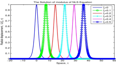
Figure 2: The solution of modulus of dissipative NLS equation with variable coefficient versus space τ
The solution of modulus of the dissipative NLS equation with variable coefficient (60) versus spaceτ at different timeξ is shown in Figure (2). It is shown that as timeξ increases, the initial wave propagates to the right with decreasing amplitude due to the effect of the viscosity.
−50 −40 −30 −20 −10 0 10 20 30 40 50 0.04
0.041 0.042 0.043 0.044 0.045 0.046 0.047 0.048
The Harmonic Wave Speed of Dissipative NLS Equation With Variable Coeficient
δ=0.1
δ=0.2
δ=0.3
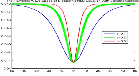
Figure 3: The speed of harmonic wave
Figure (3) illustrates the speed of harmonic wave of the dissipative NLS equation with variable coefficient versus space tau τ at different δ, where δ specify the sharpness of stenosis functionf(τ) =sech(δτ). The graph shows the speed is minimum at the center of stenosis and increases to a constant value of 0.048 as it goes away from center of stenosis. If the shape of the stenosis is sharp, the wave speed increase rapidly.
References
[1] Pedley, T.J., Fluid Mechanics of Large Blood Vessels, Cambridge University Press, Cam-bridge 1980.
[2] Fung,Y.C., Biodynamics: Circulation,Springer Verlag, New York 1981.
[3] Atabek, H.B. and Lew, H.S. Wave propagation through a viscous incompressible fluid con-tained in an initially stressed elastic tube,Biophys. J.7, 486-503, 1966.
[4] Rachev, A.J., Effects of transmural pressure and muscular activity on pulse waves in arter-ies,J. Biomech. Engng., ASME,102, 119-123, 1980.
[5] Demiray,H., Wave propagation through a viscous fluid contained in a prestressed thin elastic tube,Int. J. Eng. Sci.,30, 1607-1620, 1992.
[6] Rudinger, G., Shock waves in a mathematical model of aorta, J. Appl. Mechanics, 37, 34-37, 1970.
[7] Ling, S.C. and Atabek, H.B., A nonlinear analysis of pulsatile blood flow in arteries,J.Fluid Mech.55, 492-511, 1972.
[8] Anliker, M., Rockwell, R. L. and Ogden, E., Nonlinear analysis of flow pulses and shock waves in arteries,Z. Angew. Math. Phys. 22, 217-246, 1968.
[9] Tait, R.J., and Moodie, T.B., Waves in nonlinear fluid filled tubes, Wave Motion, 6, 197-203, 1984.
[10] Johnson, R.S., A nonlinear equation incorporating damping and dispersion, J. Fluid Me-chanics,42, 49-60, 1970.
[11] Hashizume,Y., Nonlinear pressure waves in a fluid-filled elastic tube, J. Phys. Soc. Japan.
54, 3305-3312, 1985.
[12] Yomosa, S., Solitary waves in large blood vessels,J. Phys. Soc. Japan,56, 506-520, 1987. [13] Demiray, H., Solitary waves in initially stressed thin elastic tubes,Int. J. Non-Linear Mech.,
32, 1165-1176, 1997.
[14] Antar, N., and Demiray, H., Weakly nonlinear waves in a prestressed thin elastic tube containing a viscous fluid,Int. J. Eng. Sci.,37, 1859-1876, 1999.
[15] Demiray, H., Nonlinear waves in a prestressed elastic tube filled with a layered fluid, Int. J. Eng. Sci.,40, 713-726, 2002.
[16] Tay, K. G., Forced Korteweg-de Vries equation in an elastic tube filled with an inviscid fluid.Int. J. Eng. Sci., 44, 621-632, 2006.
[17] Tay, K. G., Ong, C. T. and Mohamad, M. N., Forced perturbed Korteweg-de Vries equation in an elastic tube filled with a viscous fluid.Int. J. Eng. Sci.,.45, 339-349, 2007.
[18] Tay, K. G. and Demiray, H., Forced Korteweg-de Vries-Burgers equation in an elastic tube filled with a variable viscosity fluid.Soliton, Choas, Fractal.38, 1134-1145, 2008.
[19] Ravindran, R. and Prasad, P., A mathematical analysis of nonlinear waves in a fluid-filled viscoelastic tube, Acta Mech.31, 253-280, 1979.
[20] Antar, N., and Demiray,H., Non-linear wave modulation in a prestressed fluid field thin elastic tube,Int. J. Nonlinear Mech.34, 123-138, 1999.
[21] Demiray,H., Modulation of nonlinear waves in a a thin elastic tube filled with a viscous fluid,Int.J. Eng.Sci 37, 1877-1891, 1999.
[22] Demiray,H., Modulation of non-linear waves in a viscous fluid contained in an elastic tube,
Int.J. Nonlinear Mech.36, 649-661, 2001.
[23] Jeffrey A., Kawahara T., Asymptotic methods in nonlinear wave theory. Boston: Pitman: 1981.
[24] Prandtl, L., and Tietjens, O.G., Applied Hydro- and Aeromechanics, Dover, New York, 1957.
[25] Demiray, H., On the elasticity of soft biological tissues,J. Biomechanics,5, 309-311, 1972. [26] Demiray, H., Large deformation analysis of some basic problems in biophysicsBull. Math.
Biology,38, 701-711, 1976.
[27] Simon, B.R., Kobayashi, A.S., Stradness, D.E. and Wiederhielm, C.A., Re-evaluation of arterial constitutive laws,Circulation Research,30, 491-500, 1972.