DOI: 10.1590/1678-476620151054505522
Small mammal distributional patterns in Northwestern Argentina
María L. Sandoval1, Tania Escalante2 & Rubén Barquez1
1. Programa de Investigaciones de Biodiversidad Argentina (PIDBA), Facultad de Ciencias Naturales e Instituto Miguel Lillo, Universidad Nacional de Tucumán, Miguel Lillo 205, San Miguel de Tucumán, CP 4000, Tucumán, Argentina; Consejo Nacional de Investigaciones Científicas y Técnicas (CONICET), Argentina. ([email protected])
2. Grupo de Biogeografía de la Conservación, Departamento de Biología Evolutiva, Facultad de Ciencias, Universidad Nacional Autónoma de México. Circuito Exterior s/n, Ciudad Universitaria, Coyoacán, 04510 México, D. F., México.
ABSTRACT. Quantitative evaluations of species distributional congruence allow evaluating previously proposed biogeographic regionalization and even identify undetected areas of endemism. The geographic scenery of Northwestern Argentina offers ideal conditions for the study of distributional patterns of species since the boundaries of a diverse group of biomes converge in a relatively small region, which also includes a diverse fauna of mammals. In this paper we applied a grid-based explicit method in order to recognize Patterns of Distributional Congruence (PDCs) and Areas of Endemism (AEs), and the species (native but non-endemic and endemic, respectively) that determine them. Also, we relate these distributional patterns to traditional biogeographic divisions of the study region and with a very recent phytogeographic study and we reconsider what previously rejected as ‘spurious’ areas. Finally, we assessed the generality of the patterns found. The analysis resulted in 165 consensus areas, characterized by seven species of marsupials, 28 species of bats, and 63 species of rodents, which represents a large percentage of the total species (10, 41, and 73, respectively). Twenty-five percent of the species that characterize consensus areas are endemic to the study region and define six AEs in strict sense while 12 PDCs are mainly defined by widely distributed species. While detailed quantitative analyses of plant species distribution data made by other authors does not result in units that correspond to Cabrera’s phytogeographic divisions at this spatial scale, analyses of animal species distribution data does. We were able to identify previously unknown meaningful faunal patterns and more accurately define those already identified. We identify PDCs and AEs that conform Eastern Andean Slopes Patterns, Western High Andes Patterns, and Merged Eastern and Western Andean Slopes Patterns, some of which are re-interpreted at the light of known patterns of the endemic vascular flora. Endemism do not declines towards the south, but do declines towards the west of the study region. Peaks of endemism are found in the eastern Andean slopes in Jujuy and Tucumán/ Catamarca, and in the western Andean biomes in Tucumán/Catamarca. The principal habitat types for endemic small mammal species are the eastern humid Andean slopes. Notwithstanding, arid/semi-arid biomes and humid landscapes are represented by the same number of AEs. Rodent species define 15 of the 18 General Patterns, and only in one they have no participation at all. Clearly, at this spatial scale, non-flying mammals, particularly rodents, are biogeographically more valuable species than flying mammals (bat species).
KEYWORDS. Chiroptera, Didelphimorphia, distributional congruence, geographical patterns, Rodentia.
RESUMEN. Patrones de endemicidad de pequeños mamíferos en el Noroeste de Argentina. Las evaluaciones cuantitativas de congruencia distribucional de las especies permiten comparar regionalizaciones biogeográficas propuestas previamente e incluso identificar áreas de endemismo que no han sido detectadas. El escenario geográfico del Noroeste Argentino ofrece condiciones ideales para el estudio de patrones de distribución de especies. En este artículo aplicamos un método explícito basado en cuadrículas con el objetivo de reconocer Patrones de Congruencia Distribucional (PDCs) y Áreas de Endemismo (AEs), así como las especies (nativas pero no endémicas y endémicas, respectivamente) que las determinan, para examinar las relaciones de las especies de micromamíferos con las principales unidades ambientales. Adicionalmente, relacionamos estos patrones distribucionales con las divisiones biogeográficas tradicionales de la región estudiada y con un estudio fitogeográfico muy reciente y reconsideramos lo que previamente rechazamos como ‘áreas espurias’. Finalmente, evaluamos la generalidad de los patrones encontrados. El análisis resultó en 165 áreas consenso, caracterizadas por siete especies de marsupiales, 28 especies de murciélagos y 63 especies de roedores, lo que representa un gran porcentaje del total de especies (10, 41 y 73, respectivamente). Veinticinco por ciento de las especies que caracterizan las áreas consenso son endémicas a la región estudiada y definen seis AEs en sentido estricto, mientras que 12 PDCs están principalmente definidos por especies ampliamente distribuidas.Mientras que los análisis cuantitativos de la distribución de especies de plantas no resultan en unidades que coincidan con las divisiones fitogeográficas de Cabrera a esta escala espacial, los análisis de la distribución de especies animales muestran patronesque sí se corresponden con tales divisiones. Identificamos patrones de distribución de la fauna significativos y definimos más adecuadamente aquellos ya identificados. Identificamos PDCs y AEs que conforman los Patrones de las Pendientes Andinas del Este, los Patrones Andinos Altos del Oeste y los Patrones de las Pendientes Andinas Este y Oeste Fusionados, algunos de los cuales son re-interpretados a la luz de patrones conocidos de la flora vascular endémica. El endemismo no declina hacia el sur, pero sí hacia el oeste de la región estudiada. Los picos de endemismo se encuentran en las pendientes del este de los Andes en Jujuy y Tucumán/Catamarca, y en los biomas andinos del oeste en Tucumán/Catamarca. El tipo de hábitat principal para las especies endémicas de mamíferos pequeños está en las pendientes húmedas del este de los Andes. A pesar de esto, los biomas áridos y semiáridos y los paisajes húmedos están representados por el mismo número de AEs. Las especies de Rodentia definen 15 de los 18 Patrones Generales (GPs), y sólo en uno de ellas no participaron. Claramente, a esta escala espacial, los mamíferos no voladores, particularmente los roedores, son biogeográficamente más valiosos que los mamíferos voladores.
PALABRAS CLAVE. Chiroptera, congruencia distribucional, Didelphimorphia, patrones geográficos, Rodentia.
An area of endemism (AE) is defined by the congruent geographical distribution of 2 or more species that are spatially restricted to this area (Platnick, 1991). This means that the non-random distributional congruence of two or more species results in an AE (Crisci et al., 2006).
This definition implies sympatry, but not necessarily an
records) of the species (Murguía & Llorente-Bousquets,
2003). Several methods for identifying AEs proposed in
recent years are based on Platnick (1991)’s definition.
However, most methods traditionally applied to recognize
AEs are non-spatially explicit. Conversely, Szumik et al. (2002) and Szumik & Goloboff (2004) formalized a method that explicitly considers the spatial aspects of species distribution to identify AEs, evaluating the degree of overlap between the geographical distributions of species through the application of an optimality criterion (Szumik & Roig-Juñent 2005).
Northern Argentina is a transition zone between the tropics and subtropics: the Tropic of Capricorn passes
through Jujuy, Salta, and Formosa provinces in the north.
Due to its tropical-subtropical location, Northwestern
Argentina (NWA) provides a good opportunity to
investigate some of the factors that can determine the distribution of species. The boundaries of a diverse group of biomes converge in a relatively small region, which also
includes a diverse fauna of mammals. Moreover, NWA
includes the largest portion of the southern central Andes, whose endemic vascular plant species distribution has been recently studied (Aagesenet al., 2012). In this sense,
the geographic scenery of NWA offers ideal conditions
for the study of distributional patterns of animal species
and for comparisons between floral and faunal patterns. Also, specifically dealing with small mammals, the large
phylogenetic divergence between the three orders that
inhabit NWA allows testing the generality of the patterns
found (in the present and in previous studies, particularly those of Sandoval et al., 2010 and Sandoval & Ferro, 2014) and their transcendence to a small group of certain forms of life (i.e. a particular genus, family, order).
Although some studies have characterized the
major South American and Argentinean biomes, including those represented in NWA, as distinctive biogeographic
provinces (Cabrera & Willink, 1973; Cabrera, 1976;
Vervoorst, 1979; among others), these characterizations
were traditionally essentially qualitative, and most were based almost exclusively on its floristic components.
For example, regarding the study of Cabrera (1976),
which is almost invariably used by researchers working
in Argentina when they need to assign the study area or
flora to a phytogeographic unit, it proposes a hierarchical partition of the regions. However, the partition criteria Cabrera effectively applied is not explicit, and, although
the author argues that he categorizes successive levels of the phytogeographic hierarchy by endemism and taxa predominance, in fact, the criteria are not exclusively taxonomic and are not always hierarchically applied (Ribichich, 2002). To characterize phytogeographical areas, the author refers to the extension of the types
of vegetation, and to “what taxa of different ranks are alternately dominant, conspicuous, unique, important, frequent, endemic, dominant, abundant, distinctive,
prominent, present, common, constant, typical, represented, accompanying, associated or co-dominant in the represented
area or ecological communities” (Ribichich, 2002), without
presenting any formal definition of the meaning of such
terms. In particular, Cabrera does not clarify what concept or what synonyms of endemic he used (Ribichich, 2002).
For other than floristic taxa, with very few exceptions
(e.g., DíazGómez, 2007; Lizarralde & Szumik, 2007;
Aagesen et al., 2009; Navarro et al., 2009; Sandoval et al., 2010; Szumik et al., 2012; Sandoval & Ferro, 2014), these regions have been assumed as natural, and its congruence with the distribution of species was not tested.
In fact, quantitative evaluations of species distributional
congruence are very recent compared to narrative biogeographic regionalizations that have been made for
decades by different naturalists. Quantitative approaches
allow assessing previously proposed biogeographic regionalization and even identify previously undetected areas of endemism.
It has been previously assessed the classic
phytogeographic regionalization of NWA by using small
mammal distributional records (Sandoval et al., 2010;
Sandoval & Ferro, 2014) and the authors have been able to relate the obtained patterns to the traditional phytogeographic units within the region and to conclude that obtained distribution patterns in general concur
with those units. However, in both cases they miss the
opportunity of: (1) Analyzing the results obtained from mammal distributional data with those obtained by
Aagesen et al. (2012) in order to outline a more general biogeographical scheme for the region, i.e., an scheme
that take into account both faunal and floristic elements. (2) To deeply discuss what previous works discarded as
‘spurious’ areas (i.e., patterns that merge highly divergent units, e.g., merging eastern and western Andean slopes, or humid and arid habitats; Sandoval & Ferro, 2014), considering that some of these ‘spurious’ areas may even include a higher portion of endemic species than the areas of endemism (AEs) that they did recognize (Sandoval &
Ferro, 2014) and that some of these areas may also survive
changes in grid size (one of the identified criterions for
areas support; Aagesen et al., 2009; Casagranda et al., 2009; Szumik et al., 2012; DaSilva et al., 2015). Since AEs may or may not include a single biogeographic unit
(e.g., the endemic flora of the region do not; Aagesen
et al., 2012), we want to reassess the issue but seriously analyzing the AEs that were previously dismissed as spurious (Sandoval & Ferro, 2014). And (3) To address all small mammal distributional records in an integrated and comparative analysis to evaluate the distributional
patterns of non-flying (i.e. marsupials and rodents) versus the patterns of flying small mammals (i.e. bats) (assessment
outlined in Sandoval et al., 2010). Bats and terrestrial small mammals (marsupials and rodents) exhibit disparate
attributes, making them ideal for comparative purposes. Many bats have extensive ranges (Lyons & Willig, 1997). Actually, it has been mentioned that there is an apparently common pattern of low rates of endemism in several birds
versus non-flying vertebrates (Myers & Wetzel, 1983). Contrary, most marsupials and rodents have relatively
restricted ranges, probably due to their lack of vagility
and poor dispersal abilities.
In this paper, we applied a grid-based explicit method to analyze distributional records of Northwestern Argentinean small mammal species in order to recognize patterns of species co-occurrence and the species that determine them. Also, we relate these distributional patterns to traditional biogeographic divisions of the study region and with a very recent phytogeographic study (Aagesen et al., 2012), and we reconsider what was previously rejected as ‘spurious’ areas (Sandoval & Ferro, 2014). Finally, we assessed the generality of the patterns found by evaluating
the distributional patterns of non-flying versus the patterns of flying small mammals.
MATERIAL AND METHODS
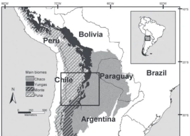
Study region. The study region is located in the southern part of the central Andes. The tropical eastern slopes of the Andes are recurrently recognized as a continental and global hotspot of diversity and endemism for several taxa (e.g., Rahbek & Graves, 2001; Barthlott et al., 2005; Kier et al., 2005; Orme et al., 2005; Sklenář et al., 2011; Patterson et al., 2012). The study region is located where the high diversity and endemism of the eastern Andes slopes gradually fade southward and
comprises the northwestern portion of Argentina (NWA), including the political provinces of Jujuy, Salta, Tucumán, Catamarca, and Santiago del Estero (Fig. 1), between parallels ~22°S and ~30°S, and meridians ~62°W and ~69°W (Fig. 1). The entire region comprises 470,184 km2, which represents approximately 17% of the total
Argentinean territory (2,791,810 km2).
Due its location between the tropical and subtropical latitudes and the complex relief, with the Andean orography on the western half of the region, which varies between 500 and 6000 m altitude, this region is characterized by
high environmental heterogeneity, great climatic contrasts
and a mosaic of different biomes. All these biomes come
together and some of them reach their limits of distribution in the region (Cabrera & Willink, 1973; Cabrera, 1976;
Burkart et al., 1999; Morrone, 2001a).
The biogeographic description outlined below follows Cabrera (1976), Burkart et al. (1999) and
Morrone (2001a). The mountain ranges are located to
the west and they are oriented north to south. The Sierras Subandinas, the Sierras Pampeanas, the Cordillera Oriental,
and the Cordillera de los Andes are the substrate on which
are developed the biomes of High Andes, Puna and Prepuna;
while on its slopes and intermountain valleys are developed
the xeric scrublands of the Monte, the montane rainforest
of the Yungas, and the semiarid woodlands of the Chaco.
The Sierras Subandinas and Pampeanas show an insular
form and are surrounded by forests of Yungas and Chaco. The other mountain systems are relatively continuous, reach higher altitudes and separate the forest environments
on the eastern slope of the open environments of Monte, Prepuna, Puna, and High Andes on the tops and the western
slope. The eastern plains correspond to the Chaco biome.
Data set. The taxonomic treatment used herein basically follows that outlined in Wilson & Reeder (2005) and Barquez et al. (2006). We used distributional information of 124 small mammal species (10 species of Didelphimorphia, 41 of Chiroptera, and 73 species
of Rodentia), i.e., those species whose adults range in weight from four grams to two kilograms (Wilson et al. 1996) and inhabits North-western Argentina (Appendix
and Supplementary Material).
The main source of data was the specimens reviewed in all the major systematic collections of Argentina (see
Acknowledgements). We also completed the data including
published localities of occurrence for small marsupials and bats, and for species of the rodent families Chinchillidae,
Caviidae, Octodontidae, and Abrocomidae (Díaz &
Barquez, 2007; Díaz et al., 2000; Jayat et al., 2009;
Jayat et al., 2013; Jayat & Ortiz, 2010; Mares et al., 1997), which have very few specimens based records and have no major problems with their alpha taxonomy. The complexity of the taxonomic history of most other species
of Rodentia and the variety of approaches taken by different authors as to the limits of each taxa make very difficult to
compare the entities mentioned in the literature with those considered in this paper.
Localities were taken from museum tags or from collector catalogues. All localities were checked and
geo-referenced using gazetteers, maps, or satellite images and
field trips. We agree with Tabeni et al. (2004) in the use
of georeferenced records to optimize the quality of the
analysis, contrary to the use of distributional maps for the species, which tend to overestimate species diversity in the regions under study (but see Soberón et al., 2000).
Finally, we divided the species into two classes according to its distributional range, restricted to the study region and widely distributed.
Distributional analyses. The method used to identify the AEs and Patterns of Distributional Congruence (PDCs) of small mammals in Northwestern Argentina was proposed by Szumik et al. (2002) and Szumik & Goloboff (2004). This method implements an optimality criterion that explicitly considers the spatial location of the species in the study region. The study region is divided into cells, and the sets of cells (=candidate areas; Aagesen et al., 2013) are evaluated through an index of endemicity. Individual values of endemicity between 0 and 1 are calculated for
each species depending on the fit of the species geographical
distribution to the candidate area being evaluated. Individual values are combined for all the species that contribute to a set to obtain the value of endemicity (score) of the area. The analysis results in a number of areas with maximum scores. This optimality criterion is implemented in the
computer program NDM and its viewer VNDM (Goloboff,
2005; available at http://www.lillo.org.ar/phylogeny/). As Sandoval & Ferro (2014), we will consider basically
two areas categories: areas of endemism (AEs, defined
only or mostly by sympatric endemic species) and local
patterns of distributional congruence (PDCs, defined only
or mostly by sympatric species not endemic to the study region). It should be noted that the optimality criterion that was used is based on the classic concept of areas of endemism. Therefore, ideally, the taxa to be used in such an analysis of endemism should be those that are maximally endemic, i.e., those whose geographic ranges are smaller than the study region. Even so, the method can be extended to be applied in the search for patterns of distributional congruence determined both by species of restricted ranges (i.e., AEs) as by widely distributed species whose ranges exceed the study region (Aagesen et al., 2009), which will constitute local patterns of distributional congruence
(PDCs) but not AEs in strict sense. While AEs in strict sense
provide strong basis for biogeographic regionalization,
PDCs provide first-step testable hypotheses of AEs for
future analyses of neighbouring regions or analyses at more inclusive scales (Szumik et al., 2012). The distributional congruence of non-endemic species may be representing parts of larger AEs, local co-occurrence by particular combinations of ecological or climatic factors, or an artifact due to unevenness of sampling localities. It is beyond the purposes of this study to identify the causal factors of
the distributional concordances identified. Whether the
factors restricting the species ranges are a combination of present day ecological and physical phenomena or
consequence of a history of vicariance and speciation, it is not a prerequisite for the detection of the pattern, which is, in turn, the first step in the elucidation of the
process generating them (Sandoval & Ferro, 2014). As
Aagesen et al. (2009), we use the optimality criterion to analyze species distribution in a regional context while relaxing the criterion of endemism. Accordingly, we will treat the scoring species as characterizing and not always as endemic species: the scoring species may be involved in the characterization of an area being or not being endemic
or exclusive to that area.
We performed analyses with five different databases:
first, one with a dataset that comprises all the small
mammal species (SM database, 124 species); then, with
a dataset that comprise terrestrial small mammals (orders
Didelphimorphia and Rodentia; TSM, 83 species); and finally, three analyses, each comprising the species of Didelphimorphia, Chiroptera, and Rodentia separately (Di, 10 species, Ch, 41 species, and Ro, 73 species). Because
there is no formal argument to use only one grid cell size (Aagesen et al., 2009; Casagranda et al., 2009), we analyzed the matrix of georeferenced data using grid cells
of four different sizes (1, 0.75, 0.5, and 0.25°
latitude-longitude). The use of several grid sizes increases the
chance of finding different areas given the topographical
complexity of the study region; moreover, using several
grid sizes provides some kind of measure of support for
a particular area of endemism: those areas which survive changes in grid size can be considered more strongly and clearly supported by the data (Aagesen et al., 2009;
Casagranda et al., 2009; Szumik et al., 2012; DaSilva et al., 2015; although some very restricted areas can be strongly supported by the data, but would not be found by larger grids; Augusto Ferrari, com. pers.). Additionally, grid sizes used in this analysis were already used for the study region facilitating comparisons with previous studies (e.g.,
Aagesen et al., 2009; DíazGómez, 2007; Navarro et al., 2009; Sandoval et al., 2010; Sandoval & Ferro, 2014;
Szumik et al., 2012). If the cells are too small the number
of artificially empty cells increases and reduce the number
of sympatric species, preventing correct detection of AEs.
The practical problem with fine grids is that available data
are usually incomplete including many gaps. To counteract
this, we established filling values, which minimize the
number of empty cells (Arias et al., 2011; Casagranda et al., 2009; Szumik & Goloboff, 2004). Therefore, we
analyzed our matrix considering different filling values for assumed and inferred presences for smaller cells (square
cells of 0.5° and 0.25° per side; Tab I). An assumed presence implies that, even if a species has not been recorded in
a cell, its presence, although unconfirmed, is suspected
or assumed by the user due to its proximity to records in neighbouring cells (Szumik & Goloboff, 2004). An inferred presence is implemented by the method itself when a species is absent from a cell but present in surrounding cells (Szumik & Goloboff, 2004). Therefore, as Szumik &
Goloboff (2004) highlighted, the assumed presences are given prior to the analysis, whereas the inferred presences
are postulated as part of the analysis. Not setting filling
values for the analysis of data when using grids with larger cell sizes is based on the fact that density of points of occurrence in relation to the proportion of the study region
that is covered by a cell of large size makes it unnecessary. For a brief explanation on how the algorithm works see Aagesen et al. (2009).
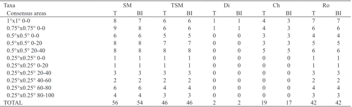
Tab. I. Results of the endemicity analysis on data set from different taxa of small mammals (SM, small mammals; TSM, terrestrial small mammals; Ch, Chiroptera; Di, Didelphimorphia; Ro, Rodentia). The total number of consensus areas obtained by using different search (analytical) parameters (i.e., cell sizes and filling values; T) and the number of biogeographically informative areas (BI, or areas not almost equivalent to the study area, see main text) as a subset of the first are indicated. Cell sizes (in degrees) and filling values (first value: assumed presences, second value: inferred presences) are also indicated.
Taxa SM TSM Di Ch Ro
Consensus areas T BI T BI T BI T BI T BI
1°x1° 0-0 8 7 6 6 1 1 4 3 7 7
0.75°x0.75° 0-0 9 8 6 6 1 1 4 3 6 6
0.5°x0.5° 0-0 6 6 5 5 0 0 3 3 4 4
0.5°x0.5° 0-20 8 8 7 7 0 0 3 3 5 5
0.5°x0.5° 20-40 8 8 8 8 0 0 5 5 6 6
0.25°x0.25° 0-0 1 1 1 1 0 0 0 0 1 1
0.25°x0.25° 0-20 1 1 1 1 0 0 0 0 1 1
0.25°x0.25° 20-40 3 3 3 3 0 0 0 0 3 3
0.25°x0.25° 40-60 2 2 2 2 0 0 0 0 2 2
0.25°x0.25° 60-80 6 6 4 4 0 0 0 0 4 4
0.25°x0.25° 80-100 4 4 3 3 0 0 0 0 3 3
TOTAL 56 54 46 46 2 2 19 17 42 42
through a heuristic search and default NDM parameters: searching groups of cells by adding/eliminating one cell at a time, and saving groups defined by two or more endemic species and with scores higher or equal to 2.0. Groups of
cells with more than 50% of species in common were ruled out retaining those with highest scores, and groups of cells
with a score up to 1% inferior were stored in memory. We
obtained consensus areas using the loose consensus rule
in VNDM (see Aagesen et al., 2013).
The distributional patterns were evaluated in the context of traditional biogeographic divisions by plotting
the distribution of the defining species upon the terrestrial eco-regions as defined by Burkart et al. (1999) and Olson et al. (2001). The results were mapped using the program
Global Mapper v11.02. Finally, all consensus areas were grouped in General Patterns (GPs) employing a qualitative
criterion (see DaSilva et al., 2015), according to their fit to the traditional biogeographic divisions considered.
RESULTS
We reviewed a total of 8,673 specimens, and we identified 8,400 of them to the species level. From these,
8,117 had precise punctual localities and represented 119
of the 124 NWA species included in this work (Appendix).
Altogether, the principal database contains 11,596
geo-referenced records of 124 of the 128 known NWA small
mammal species [exceptions are Necromys amoenus (Thomas, 1900), Oxymycterus akodontius Thomas, 1921, Graomys edithae Thomas, 1919, and Ctenomys fochi Thomas, 1919].
The results we obtained by analyzing data from
the different taxa of small mammals are summarized in
Tables I to IV. The analysis resulted in 165 consensus areas.
Four large areas almost equivalent to the study region
were not considered in the following characterization (see Discussion). The remaining 161 areas represent PDCs or AEs in strict sense characterized by 7 species of marsupials, 28 species of bats, and 63 species of rodents.
Thirty-two species (25% of all study region small mammal fauna that characterize consensus areas) are
endemic to the study region and define six GPs that are AEs in strict sense (Tab. III). Other 12 GPs are mainly defined by
widely distributed species (whose distributions exceed the
study region) and therefore we consider these GPs as PDCs. Of all the 18 GPs, 6 (3 of the AEs in strict sense and 3 PDCs)
run transversal to the Andes, in an east-west direction, and group together eastern and western Andean biomes, joining up lowland and moist or dry highland species
(Figs 14-19). On the other hand, the other 9 PDCs run
parallel to the Andes, in a north-south direction, including eastern or western Andean biomes (Figs 2-10). The other 3 AEs are located in the south of the study region, either on the eastern moist Andean slopes and lowlands or on the
western dry valleys (Figs 11-13). Of the 18 GPs, 6 were previously identified (Sandoval & Ferro, 2014). The other 12 are novel distributional congruence patterns or
are more detailed or precise definitions of some patterns previously outlined. Since the characterization of the GPs
already reported by Sandoval & Ferro (2014) is basically the same, the new characterization is not included in the
following statement. The number of areas equivalent to each of such GPs, the databases and cell sizes of the grids that allowed their identification, and the number, identity and distributional fit of the characterizing species are provided
in Figs. 2-7, and in Tables II and III.
Local Patterns of Distributional Congruence
1.Widespread Eastern Andean Slopes (“Argentinean Yungas”) (already obtained by Sandoval & Ferro, 2014; Fig. 2).
2.North-eastern Andean Slopes (“Northern Argentinean Yungas”) (already obtained by Sandoval & Ferro, 2014; Fig. 3).
Andean Slopes pattern. This PDC were only obtained
analyzing the SM database with the smallest grid sizes
(Tab. II). Three species characterize this PDC. There is one endemic species characterizing these areas (Tab. III).
4.Eastern Andean Slopes and Lowlands (“Argentinean Yungas and Chaco”) (Fig. 5). Two consensus areas were
equivalent to this pattern. This PDC were obtained only
analyzing the Ch database (Tab. II). Fifteen species characterize this PDC. There are none endemic species characterizing these areas (Tab. III).
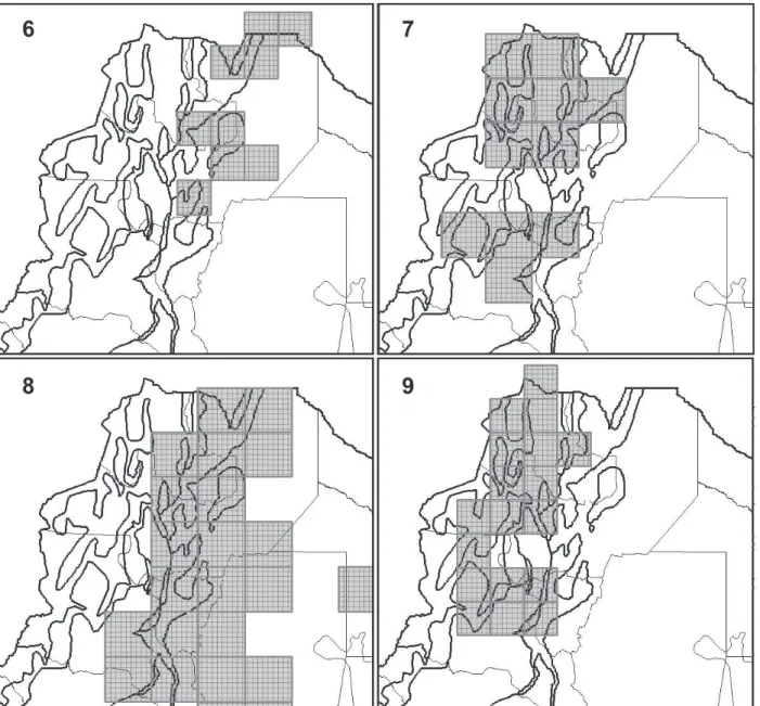
5. North-eastern Andean Slopes and Lowlands (“Northern Argentinean Yungas and Chaco”) (Fig. 6). Six
consensus areas were equivalent to this pattern. This PDC were obtained analyzing the SM, TSM, and Ro databases with big grid sizes (Tab. II). Twenty-five
species characterize this PDC. There are nine endemic species characterizing these areas (Tab. III).
6. Mountain Tops and Western Andean Slopes (“Northern Argentinean Highlands”) (Fig. 7). Three consensus
areas were equivalent to this pattern. This PDC were only obtained analyzing the TSM and Ro databases
with large grid sizes (Table 2). Nine widely distributed species characterize this PDC (Tab. III).
7.Eastern Lowlands (“North-western Argentinean Chaco”)
(Fig. 8). Two consensus areas were equivalent to this
pattern. This PDC were only obtained analyzing the
TSM and Ro databases with the biggest grid sizes
(Tab. II). Four widely distributed species characterize this PDC (Tab. III).
8. Widespread Western High Andes (“Puna”) (already obtained by Sandoval & Ferro, 2014; Fig. 9). 9.North-western High Andes (“High Andes”) (already
obtained by Sandoval & Ferro, 2014; Fig. 10). 10.Eastern Andean Slopes merged with Western Andean
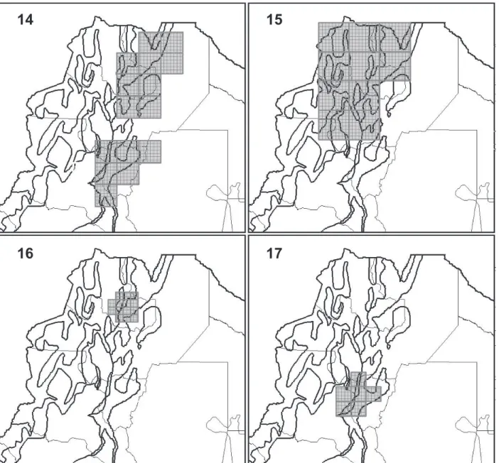
Biomes (E-W): The combination of Argentinean Yungas, Chaco, and Monte (Fig. 14). Two latitudinally extensive consensus areas were obtained in the study region (Tab. II). These areas were characterized by 23 species
(Tab. III). Of these, 16 species correspond to the moist
eastern slopes and lowlands, and 7 [E. patagonicus Thomas, 1924, L. blossevillii (Lesson & Garnot, 1826), N. macrotis (Gray, 1839), S. lilium (E. Geoffroy
Saint-Hilaire, 1810), C. tschudii Fitzinger, 1857, O. flavescens
(Waterhouse, 1837), and P. osilae J. A. Allen, 1901] inhabit both the western arid slopes and the eastern biomes.
11.North-eastern Andean Slopes merged with Northwestern Andean Biomes I (NE-NW): The combination of Argentinean Yungas and Puna (Fig. 15). Three big consensus areas were obtained in the north of the study region (Tab. II). These areas were characterized by nine species (Tab. III). There are two endemic species (Tab. III). All characterizing species can be divided in two sets; a highland group of species [A. albiventer Thomas, 1897, A. boliviensis Meyen, 1833, E. hirtipes (Thomas, 1902), E. puerulus (Philippi, 1896), and O.
gliroides (Gervais & d’Orbigny, 1844)] and a lowland or sylvan set [A. budini (Thomas, 1918), M. keaysi J. A. Allen, 1914, O. paramensis Thomas, 1902, and T.
wolffsohni Thomas, 1902].
12. eastern Andean Slopes merged with North-western Andean Biomes II (NE-NW): A patch of High Andes, Puna, Monte, and Yungas in Jujuy province: Finca Las Capillas and nearby fragment of Sierra de Tilcara (Fig. 16). Ten small consensus areas were obtained in the north of the study region (Tab. II). These areas were characterized by nine species (Tab. III). There are two endemic species (Tab. III). All characterizing species can be divided in two sets; a highland group of species [A. jelskii (Thomas, 1894), A. sublimis (Thomas, 1900), C. budini Thomas, 1913, N. ebriosus Thomas, 1894, and P. caprinus Pearson, 1958) and a lowland or sylvan set [E. chiriquinus Thomas, 1920, H. velatus (I. Geoffroy Saint-Hilaire, 1824), M. rufus E. Geoffroy Saint-Hilaire, 1805, and T. primus Anderson & Yates, 2000].
Areas of Endemism
13. South-eastern Andean Slopes (“Southern Argentinean Yungas”) (already obtained by Sandoval & Ferro, 2014; Fig. 11).
14.South-eastern Andean Slopes and Lowlands (“Southern Argentinean Yungas and Chaco”) (Fig. ). Twenty-four
consensus areas were equivalent to this pattern. This AE were obtained analyzing the SM, TSM, and Ro
databases with small grid sizes (Tab. II). Eight species characterize this AE. There are six endemic species characterizing these areas (Tab. III).
15. South-western High Andes (“Monte Desert”) (already obtained by Sandoval & Ferro, 2014; Fig. 13). 16. eastern Andean Slopes merged with
South-western Andean Biomes I (SE-SW): The combination of Argentinean Yungas and Monte (Fig. 17). Twelve
consensus areas were equivalent to this GP. This AE was obtained analyzing the SM, TSM, and Ro databases
with almost all grid sizes (except the biggest one).
Ten species characterize this AE (Tab. III). Of these,
three species correspond to the western arid slopes [E. bolsonensis Mares, Braun, Coyner & Van Den Bussche, 2008, E. moreni (Thomas, 1896), and R. auritus (G. Fischer, 1814)] and seven to the moist eastern slopes. There are nine endemic species.
17. eastern Andean Slopes merged with South-western Andean Biomes II (SE-SW): The combination of Argentinean Yungas, Chaco, and Monte (Fig. 18).
Ten consensus areas were equivalent to this GP. This AE was obtained analyzing the SM, TSM, and Ro
databases with almost all grid sizes (except the smallest
one). Nineteen species characterize this AE. Of these,
the western arid slopes and the eastern biomes. There are 16 endemic species (Tab. III).
18. eastern Andean Slopes merged with South-western Andean Biomes III (SE-SW): The combination of Argentinean Chaco and Monte (Fig. 19). Three
consensus areas were equivalent to this GP. This
AE was obtained analyzing the SM, TSM, and Ro
databases with a moderate grid size. Three endemic species characterize this AE (Tab. III), of which one correspond to the western arid slopes (P. aureus Mares,
Braun, Barquez, & Díaz, 2000) and the other two inhabit
both the western arid slopes and the eastern lowlands.
Tab. II. Results of the endemicity analysis on data from different data set of small mammals. The number of consensus areas obtained by analyzing data from each of the taxa considered (S, small mammals; T, terrestrial small mammals; D, Didelphimorphia; C, Chiroptera, R, Rodentia) with grids with different cell sizes (a: 1°;b: 0.75°;c: 0.5°; d: 0.25°) is shown. Filling values are not shown. The General Pattern numbers (GP) correspond to those in the text.
GP1 GP2 GP3 GP4 GP5 GP6
S T D C R S T D C R S T D C R S T D C R S T D C R S T D C R
a 1 1 1 1 1 1 1 1 1 1 1 1
b 1 2 1 1 2 1 1 1 1 1 1 1 1
c 9 7 6 5 6 7 4 4 1
d 1 2 1 1 1
To 12 10 2 8 8 9 9 0 6 6 1 0 0 0 0 0 0 0 2 0 2 2 0 0 2 0 2 0 0 1
40 30 1 2 6 3
GP7 GP8 GP9 GP10 GP11 GP12
S T D C R S T D C R S T D C R S T D C R S T D C R S T D C R
a 1 1 1 2 1
b 1 1 1 1 1
c 1
d 1 1 1 3 3 3
To 0 1 0 0 1 2 1 0 0 1 1 1 0 0 1 1 0 0 1 0 2 0 0 0 1 4 3 0 0 3
2 4 3 2 3 10
GP13 GP14 GP15 GP16 GP17 GP18
S T D C R S T D C R S T D C R S T D C R S T D C R S T D C R
a 2 2 2
b 1 1 1 1
c 1 1 1 1 1 1 2 2 2 1 1 1 1 1 1
d 1 1 1 7 7 7 1 1 1
To 1 1 0 0 1 8 8 0 0 8 1 1 0 0 1 4 4 0 0 4 4 3 0 0 3 1 1 0 0 1
3 24 3 12 10 3
Tab. III. Characterizing species of each biogeographically significant area obtained by analyzing data of different taxa under different search parameters (not shown). The numbers of the General Patterns (GP) correspond to those in the text. If the GP constitute a Local Pattern of Distributional Congruence (PDC) or an Area of Endemism in strict sense (AE) is specified. Restricted (R) and widely distributed (W) species of each GP are indicated. General Patterns GP1 GP2 GP3 GP4 GP5 GP6 GP7 GP8 GP9 GP10 GP11 GP12 GP13 GP14 GP15 GP16 GP17 GP18
Species PDC PDC PDC PDC PDC PDC PDC PDC PDC AE AE AE PDC PDC PDC AE AE AE
Cryptonanus chacoensis W W
C. ignitus R
Micoureus constantiae W W
Thylamys cinderella R R
T. pusillus W
T. sponsorius R R
T. venustus W
Anoura caudifer W W
A. planirostris W W W
Chrotopterus auritus W W W
Cynomops planirostris W W
Diaemus youngi W W
Eptesicus chiriquinus W W W
E. diminutus W W W
Eumops bonariensis W
E. glaucinus W W W W
E. patagonicus W W W
Glossophaga soricina W W
Histiotus laephotis W W W
H. macrotus W
General Patterns GP1 GP2 GP3 GP4 GP5 GP6 GP7 GP8 GP9 GP10 GP11 GP12 GP13 GP14 GP15 GP16 GP17 GP18
Species PDC PDC PDC PDC PDC PDC PDC PDC PDC AE AE AE PDC PDC PDC AE AE AE
H. velatus W W W
Lasiurus blossevillii W W W
Myotis microtis W W
M. rufus W W W
M. albescens W W W
M. keaysi W W W
M. riparius W W W
Noctilio leporinus W W
Nyctinomops laticaudatus W W W W
N. macrotis W W W
Pygoderma bilabiatum W W
Sturnira erythromos W W W
S. lilium W W W
S. oporaphilum W W W
Abrothrix andinus W W
A. illuteus R R
A. jelskii W W
Akodon albiventer W W
A. aliquantulus R
A. boliviensis W W W
A. budini R R R
A. caenosus W W
A. fumeus R R
A. simulator W
A. spegazzinii W R
A. sylvanus R R
A. toba W
Andalgalomys olrogi R R
Andinomys edax W W
Auliscomys sublimis W W
Bolomys lactens R R
B. lenguarum W
Calomys callosus W
C. lepidus W W
C. musculinus W
Cavia tschudii W W
Ctenomys budini R R
C. coludo R R
C. knighti R R
C. latro R R
C. occultus R
C. opimus W W
Tab. III. Cont.
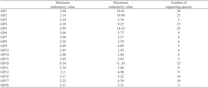
Tab. IV. Minimum and maximum endemicity values and supporting species for each General Pattern (GP). The numbers of the GPs correspond to those in the text.
Minimum endemicity value
Maximum endemicity value
Number of supporting species
GP1 2.04 19.41 36
GP2 2.14 10.98 23
GP3 2.34 2.34 3
GP4 4.28 9.25 15
GP5 2.99 14.52 25
GP6 3.06 3.77 9
GP7 2.06 2.57 4
GP8 2.26 2.59 6
GP9 4.09 4.09 5
GP13 2.45 2.45 4
GP14 2.06 2.84 8
GP15 2.05 2.05 3
GP10 8.34 11..85 23
GP11 2.74 3.86 9
GP12 2.2 4.98 9
GP16 2.17 5.22 10
GP17 2.22 6.29 19
DISCUSSION
Floristic vs faunal patterns. As highlighted by Godoy-Bürki et al. (2013), since endemism is a fundamental criterion to identify conservation areas, it is urgent that botanists and zoologists to conduct local distributional analyses, “in order to obtain an integrated
solution for protecting both the flora and fauna in the
region” (Godoy-Bürki et al., 2013). In fact, in NWA there are hotspots for vascular plants and several animal taxa, including mammals (Szumik et al., 2012). However,
knowledge on distributional patterns and endemism for this region is very uneven among different taxa.
Surprisingly, it seems that, while detailed
quantitative analyses of plant species distribution data
do not result in units that correspond to Cabrera’s phytogeographic divisions at this spatial scale (Aagesen et al., 2012), analyses of animal (here, small mammal)
species distribution data generally do. So, despite the system Cabrera used was not based on quantitative studies and did not apply consistent criteria for defining the individual
phytogeographic units (Aagesen et al., 2012), what he
observed in local and regional flora composition may be
determining animal distributions (e.g. Sandoval et al., 2010; Szumik et al., 2012; Sandoval & Ferro, 2014),
although plant endemic species distribution quantitative
analyses result in areas of endemism that do not correspond to his divisions (Aagesen et al., 2012). Although many of
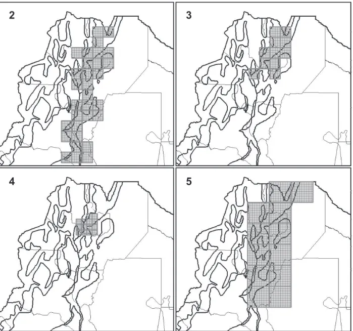
Figs 2-5. Fig. 2, a case of GP1, Widespread Eastern Andean Slopes PDC recovered through the analysis of SM database and with a grid of cells of 0.5°x0.5° and filling values of 0 for assumed presences and 20 for inferred presences. Fig. 3, a case of GP2, North-eastern Andean Slopes PDC recovered through the analysis of TSM database and with a grid of cells of 0.5°x0.5° and filling values of 0 for assumed presences and 20 for inferred presences. Fig. 4, a case of GP3, A patch of the Northern Argentinean Yungas: Finca Las Capillas PDC recovered through the analysis of SM database, with a grid of cells of 0.25°x0.25° and filling values of 80 for assumed presences and 100 for inferred presences. Fig. 5, a case of GP4, Eastern Andean Slopes and Lowlands PDC recovered through the analysis of Ch database, with a grid of cells of 1°x1° and without filling values.
2
3
the areas we obtained, both AEs and PDCs, are constituted by cells that include a wide array of habitats, the natural history and habitat preferences of the characterizing species allow us to certainly relate them to phytogeographic units
previously defined by Cabrera (Cabrera & Willink, 1973;
Cabrera, 1976).
All the obtained AEs are located in the south of the study region, either in the eastern Andean slopes and the western Andean biomes, and even in many cases those
landscapes are merged in one AE. Similarly to what happens
with vascular plants (Aagesen et al., 2012), small mammal endemic species are far from evenly distributed in the study
region. Of the 33 endemic species (Table 3), only five are
more or less latitudinally widely distributed [T. cinderella (Thomas, 1902), T. sponsorius (Thomas, 1902), B. lactens
(Thomas, 1918), G. domorum (Thomas, 1902), and M. shiptoni (Thomas, 1925)]. Interestingly, endemism, unlike what happens in vascular plants (Aagesen et al., 2012), does not declines towards the south, but does declines towards the west of the study region. Ten endemic species have their distributional ranges located in the north of the study region meanwhile 18 are in the south of the study region.
On the other hand, 23 species inhabit in environments of
eastern Andean slopes and lowlands meanwhile only ten inhabit western Andean biomes. The geographical location of our AEs and PDCs are mostly congruent with the most important hotspots for endemic vascular plant species.
Our largest GPs include almost all the endemic species hotspots defined by Godoy-Bürki et al. (2013). And there
are even coincidences at a more local scale: our GP16 Figs 6-9. Fig. 6, a case of GP5, North-eastern Andean Slopes and Lowlands PDC recovered through the analysis of TSM database, with a grid of cells of 0.75°x0.75° and without filling values. Fig. 7, a case of GP6, Mountains Tops and Western Andean Slopes PDC recovered through the analysis of TSM and Ro databases, with a grid of cells of 1°x1° and without filling values. Fig. 8, a case of GP7, Eastern Lowlands PDC recovered through the analysis of TSM database, with a grid of cells of 1°x1° and without filling values. Fig. 9, a case of GP8, Widespread Western High Andes PDC recovered through the analysis of SM, TSM, and Ro databases, with a grid of cells of 0.75°x0.75° and without filling values.
6
7
(Fig. 17) includes the Sierra del Aconquija, between the provinces of Tucuman, Salta and Catamarca, which has the
highest concentration of endemic plant species in the study region (Godoy-Bürki et al., 2013); and our GP15 (Fig.
13), which includes Andalgalá, Santa Maria, and Ambato
in Catamarca, was recognized as another important AE for plant endemism (Godoy-Bürki et al., 2013).
Endemism and co-occurrence patterns. Highest
numbers of endemic species (but not necessarily recognized
AEs) are found in the eastern Andean slopes in Jujuy and Tucumán/Catamarca, with nine and eight endemic species respectively, and in the western Andean biomes in Tucumán/ Catamarca, with eight endemic species. Of these three high
endemism sites that we a priori and qualitatively identified, our analysis was able to recover two patterns as AEs in strict sense, while the other was recovered as PDCs (which are characterized both by endemic and non-endemic species).
However, both endemism patterns are impoverished in term of defining species: in any case the recovered areas
were characterized by the complete assemblage of endemic species but only by a subset of such species (Tab. III). The South-eastern Andean Slopes pattern is an AE and
corresponds to an endemism peak. Sandoval & Ferro (2014) recovered this pattern, characterized by 14 rodent
species, 12 been endemic to the study region, been our GP
also characterized only by rodent species (but far fewer).
Figs. 10-13. Fig. 10, a case of GP9, North-western High Andes PDC recovered through the analysis of SM, TSM, and Ro databases, with a grid of cells of 0.25°x0.25° and filling values of 80 for assumed presences and 100 for inferred presences. Fig. 11, a case of GP13, South-eastern Andean Slopes AE recovered through the analysis of SM, TSM, and Ro databases, with a grid of cells of 0.25°x0.25° and filling values of 20 for assumed presences and 40 for inferred presences. Fig. 12, a case of GP14, South-eastern Andean Slopes and Lowlands AE recovered through the analysis of SM, Ch, and Ro databases, with a grid of cells of 0.25°x0.25° and filling values of 60 for assumed presences and 80 for inferred presences. Fig. 13, a case of GP15, South-western High Andes AE recovered through the analysis of SM, TSM, and Ro databases, with a grid of cells of 0.5°x0.5° and filling values of 0 for assumed presences and 20 for inferred presences.
10
11
Despite the low number of our characterizing species, this AE has a high endemicity score and repeated occurrence
(Tab. IV). This pattern corresponds to the Southern sector of the Yungas forest of NWA, which has been differentiated
by phytogeographers as an impoverished version of the
Northern sector rather than on exclusive floral elements
(Cabrera, 1976; Morales, 1996; Brown et al., 2001).
Moreover, Aagesen et al. (2012) reported that vascular
flora endemism declines gradually towards the south of the study region. However, this area was recovered for insects
(Navarro et al., 2009), for a taxonomically diverse data set
when analysed using quantitative approaches (Szumik et al., 2012), and for rodents (Sandoval & Ferro, 2014; our
study), revealing the Southern sector of the Argentinean
Yungas as a distinctive faunal AE, and, at least in the case
of endemic small mammals, not a impoverished one. On
the other hand, regarding the case of the other obtained
AE that corresponds to an endemism peak, the Monte biogeographic province in NWA was recover as and named
as the South-western High Andes pattern. This western Andean biome occurs on the arid western (rain shadow) slopes. As the Yungas forest reach its southern tip on the
humid eastern Andean slopes in NWA, the Monte province
reaches its northernmost extension on the west-faced slopes of the same mountain ranges. Also, one of the highest concentrations of endemic plant species were found mostly
Figs 14-17. Fig. 14, a case of GP10, Eastern Andean Slopes merged with Western Andean Biomes (E-W) PDC recovered through the analysis of SM and Ch databases, with a grid of cells of 0.75°x0.75° and without filling values. Fig. 15, a case of GP11, North-eastern Andean Slopes merged with Northwestern Andean Biomes I (NE-NW) PDC recovered through the analysis of SM database, with a grid of cells of 1°x1° and without filling values. Fig. 16, a case of GP12, North-eastern Andean Slopes merged with North-western Andean Biomes II (NE-NW) PDC recovered through the analysis of SM, TSM, and Ro databases, with a grid of cells of 0.25°x0.25° and filling values of 20, 40, and 60 for assumed presences and 40, 60, and 80 for inferred presences. Fig. 17, a case of GP16, South-eastern Andean Slopes merged with South-western Andean Biomes I (SE-SW) PDC recovered through the analysis of SM, TSM, and Ro databases, with a grid of cells of 0.5°x0.5° and without filling values.
14
15
Figs 18, 19. Fig. 18, a case of GP17, South-eastern Andean Slopes merged with South-western Andean Biomes II (SE-SW) PDC recovered through the analysis of SM database, with a grid of cells of 1°x1° and without filling values (Southern area; see Results). Fig. 19, a case of GP18, South-eastern Andean Slopes merged with South-western Andean Biomes III (SE-SW) PDC recovered through the analysis of SM, TSM, and Ro databases, with a grid of cells of 0.5°x0.5° and filling values of 20 for assumed presences and 40 for inferred presences.
in the High Monte environments, especially in transition zones with the Southern Andean Yungas (Godoy-Bürki et al., 2013).
Unlike to what happens with endemic vascular
plants (Aagesen et al., 2012; Godoy-Bürki et al., 2013), whose hotspots at a regional scale are concentrated in
the arid ecoregions of NOA (with 80% of the endemic flora; Aagesen et al., 2012), the principal habitat types for endemic small mammal species are not the western or eastern arid or semi-arid biomes, but the eastern humid Andean slopes, with 20 endemic species (versus 13 in arid
and semi-arid environments). Notwithstanding,
arid/semi-arid biomes and humid landscapes are represented by the
same number of AEs: one for arid/semi-arid biomes (GP15), one for humid landscapes (GP13), and four mixed GPs, which include both habitat types (GP14, 16, 17, and 18).
Contrary to our results, Aagesenet al. (2012) reported that very few vascular plant species are restricted to subhumid or humid environments in this region. They highlighted this surprising poverty in endemic species of the otherwise diverse Tucumano-Bolivian Yungas forest at a local scale. It should be noted that Aagesen et al. (2012) stressed that the mountain grasslands above the tree line were included in the Puna (following Ibisch et al., 2003), meanwhile in the phytogeographical scheme outlined by Cabrera (1976), which we follow, these grasslands are considered the highest strata of the Yungas. Notoriously, supporting Ibisch et al. (2003) scheme, we obtained the Mountain Tops and Western Andean Slopes pattern (a PDC), which, even though it represents an association between areas, apparently not correspond to a transition zone between biogeographic units but a natural unit characterized by species mostly inhabiting
all environments represented in the area. Obtaining this GP
allows formally grouping all those highlands environments
(High Andes, Puna, and mountain grasslands) that harbour
common assemblages of rodent species. This issue will
be presented in more detail in another manuscript. On
the other hand, the Widespread Eastern Andean Slopes allows us to identify the entire latitudinal extension of the Yungas forest as a discrete biogeographic unit regarding
the NWA geographic context. This is a stable pattern since it was recovered with different databases with different grid sizes (Tab. II). However, only 5 of the 36 species
that characterize the Yungas forest are exclusive or almost
exclusive of the NW Argentinean Yungas. This may well indicate that the Yungas of NWA may be part of a larger
AE extending beyond the limits of our study region: the
Yungas forest in NWA is the tail of a broader area that
extends towards the north through Bolivian Yungas and probably to southern Peru. Alternatively, the recognition of distributional congruence in the species distributions may
be due to a similar response to a unique combination of
ecological and historical factors restricting species ranges
that not necessarily affect in the same way these species
north or southwards. The recognition of this pattern was also reported for bats and marsupials (Sandoval et al., 2010) and for rodents (Sandoval & Ferro, 2014). Meanwhile, the North-eastern Andean Slopes, near the Bolivian border, is just traversed by the Tropic of Capricorn. Certainly,
the northern part is the richest sector of the NWA Yungas
forest which gradually impoverished southward (Ojeda &
Mares, 1989; Ojeda et al., 2008), althought this statement do not applies to endemic small mammal species (see above). For bats and marsupials (Sandoval et al., 2010) and for rodents (Sandoval & Ferro, 2014) the Northern sector of the Argentinean Yungas was also recovered. Contrary to the low number of endemic species found by
Sandoval & Ferro (2014) for this pattern, according to our
results, almost half of the defining species (9 of the 23) are
exclusive or almost exclusive to this PDC. Notably, even
defined as a PDC, the fact of containing several endemic
species would not allow a delimitation of an AE in the context the analyses we performed. Probably, this PDC would be obtained as an AE if distributional records of only endemic species are included in a study that do not include widespread species (Aagesen et al., 2012). In that
case, perhaps we could define a PDC and an overlapping AE, and they would belong to the same GP. However,
given that our analyses include both endemic and widely distributed species in the datasets, we can only speculate.
We identify Argentinean High Andes (North-western High Andes, GP9) and Puna (Widespread Western High Andes) provinces as discrete biogeographic units in the
geographic context of NWA. Maybe, the High Andes and the Puna of NWA are part of larger AEs extending southward
in Argentina and northward into Bolivia. For rodents (Sandoval & Ferro, 2014) the Argentinean High Andes
and Puna were also recovered. However, as for vascular
plants, the relative low number of endemic highland species is unexpected and may be underestimated as collection localities in those landscapes are scarce (Aagesen et al., 2012). As Sandoval & Ferro (2014) mentioned, large areas of these highlands remain unexplored and so further
exploration should clarify the existence of different AEs associated with mountaintops on the highlands of NWA.
Despite that, one of the highest concentrations of endemic plant species were found mostly in the Central Andean Puna environments, especially in transition zones with
the Southern Andean Yungas (Godoy-Bürki et al., 2013).
Szumik et al. (2012) were able to recover the Chaco biogeographic province but later Sandoval & Ferro (2014) failed to recognize it neither as an AE nor as a
PDC. We recovered the Chacoan biome both as hybrid
areas, mixed with the Yungas environments (the Eastern Andean Slopes and Lowlands and the nested North-eastern Andean Slopes and Lowlands and South-eastern Andean Slopes and Lowlands) and as independent areas (Eastern Lowlands, GP7). Although the scattered sampling localities
may prevent or difficult its identification as a sympatric
distributional pattern, the Chacoan small mammals, and the species inhabiting both biomes (Chaco and Yungas), allow the recognition of this biogeographic province as a PDC (see also Sandoval & Barquez (2013) for a detailed interpretation of the Chacoan bat fauna assemblages).
Finally, despite the identification of four large areas almost equivalent to the study region, we were not able to obtain a pattern equivalent to the southern part of the central Andes, which was recognized as a single AE, defined
by at least 53 species of vascular plants that are widely distributed within the study region but are endemic to it (Aagesen et al., 2012). We considered our four wider consensus areas biogeographically not informative at this spatial scale because they have a too large surface (as
mentioned, almost equivalent to the study region) and
are characterized by many widespread species, in some
cases presenting high endemicity values, all these making
impossible their interpretation at this analysis scale. In our spatial scale of analysis, these areas could be interpreted as areas that integrate transition zones, because they present
varied and complex characterizing faunas. So, it is likely
that these areas are part of a more inclusive pattern evident
to a larger scale of analysis. However, this interpretation
is purely speculative. For these reasons, those areas are not considered in this discussion.
‘Spurious’ areas? Finally, we obtained three sets
of ‘merged-unit’ areas: latitudinally extensive (GP10) and northern (GP11 and 12) and southern (GP16, 17, and
18) groupings of eastern and western Andean biomes. All these areas combine consensus areas corresponding to
well defined classic main patterns. Sandoval & Ferro (2014) interpreted these areas as ‘spurious’ areas and, as
Aagesen et al. (2013) stated, as a likely outcome of using the ‘loose’ consensus rule. The loose rule merges areas if
they share a user defined percentage of their defining species
with at least one other area in the consensus (Aagesen et al., 2013). The ‘loose’ consensus rule is a useful tool for detecting gradual overlapping distribution patterns and replacement among areas. Therefore, Sandoval &
Ferro (2014) considered that the spurious areas may well be indicating a transition zone between the main patterns
involved. Some of our ‘merged-unit’ areas actually seem
to be what Sandoval & Ferro (2014) called ‘spurious’
areas, since they more likely represent turnover gradients
rather than congruence patterns (Augusto Ferrari, com. pers.). Interestingly, Aagesen et al. (2012) do not share our view. In their analyses all areas were characterized by
species from very different altitudes that do not necessarily
strictly coexist but are founded in the same cell or cell set because in the study region several phytogeographic units are separated from each other by very short distances. They consider those AEs as valid and their high endemic areas include several environments and are characterized by vascular plant species that are not sympatric but inhabit highly altitude and aridity variable landscapes. This is the
case of GP11, 12 (both PDC), and 16 (an AE), because
in these areas species that are not sympatric at all, which
inhabits very environmentally different landscapes, are
grouped.
However, GP10 (a PDC), 17, and 18 (both AEs) include some species that are in fact sympatric. Moreover,
these areas are among the high endemic areas found when
analyzing the endemic vascular flora (Aagesen et al., 2012) and present high concentrations of endemic plant species
(especially the transition zones from the Southern Andean Yungas to the High Monte, Godoy-Bürki et al., 2013). So, interestingly, small mammals and vascular plants appear to
define the same AEs in NWA (Lone Aagesen, com. pers.). This finding is very important, especially considering
that areas with high levels of endemism are priorities for
conservation because they reflect past and potentially future
speciation events (Rosenzweig, 1995; Fa & Funk, 2007).
taxa represent essential conservation targets particularly if occurring in rather small geographic areas (Vane-Wright et al., 1991; Linder, 1995; Peterson & Watson, 1998).
Taxa. Rodent species define 15 of the 18 GPs, while bats define four and marsupials only define one. The GP defined by bats and marsupials and two defined by bats are also defined by rodents. So, only three GPs are not recovered
through the analysis of rodent species distributional data,
and even these GPs have rodent characterizing species
when analized together with all small mammal species
(GP3 and GP10). Only in GP4 rodents have no participation at all. Clearly, at this spatial scale, non-flying mammals,
particularly rodents, are bigeographically more valuable
species than flying mammals (bat species). The other
terrestrial small mammals considered (marsupials) include very few (10) and not always distributionally overlapping
species in NWA, and this is probably why they are so
little involved in the characterization of areas, compared to rodents. Therefore, as suggested by Sandoval &
Ferro (2014), rodents are very useful to analyse patterns of endemism and biographical regionalization in small geographical areas. This is probably due to the fact that a large proportion of mammals with restricted distributions
are rodents, independently of their taxonomic level (genera/
species) or spatial scale (Arita et al., 1997; Danell, 1999; Danell & Aava-Olsson, 2002), that they are present in all type of biomes from tropical moist forest
to gelid highland deserts, and that they constitute quite conspicuous assemblages as a consequence of adaptation
to environments (Mena & Vázquez-Domínguez, 2005;
Patterson et al., 1998). Moreover, rodents are the most
diverse order of mammals containing 42% of known species
(Musser & Carleton, 2005), thus frequently being the most important part of mammal assemblages concerning number of species.
Using different search (analytical) parameters.
Numerous studies support the hypothesis that the results obtained at a given spatial or temporal scale can not
necessarily be obtained or be significant at larger or
smaller scales (Lyons & Willig, 1999, and references cited therein), so it is interesting and valuable to document scale
dependence of different patterns. Casagranda et al. (2009)
analyzed the implications of using different scales of analysis
with the optimality method, recovering some patterns at all spatial scales, but also recovering certain patterns only in some particular scale. According to Laffan & Crisp (2003),
we are closer to finding a complete representation of the
true pattern of distributional congruence and endemicity varying the spatial scale of analysis than without doing it. In our analysis, the dependence of local patterns of distributional congruence and endemicity on the spatial scale does not seem to be decisive: most patterns remain
constant during the analysis at different scales (i.e., grid sizes). Our GP1 and 2 are obtained using four different grid sizes, GP16 and 17 are obtained using three different grid sizes, and GP4, 5, 6, 8, 12, and 14 are obtained using two different grid sizes (Tab. II). Distributional congruence
and endemicity patterns that do not support changes in the
cell size can be a simple artifact of a specific grid, while
resistance to changes in cell size is an important factor in assessing a particular distributional pattern (Aagesen et al., 2009). According to this framework, our GP3, 7, 9,
10, 11, 13, 15, and 18 could be artifacts of the technique without a real biogeographical significance. Considering this, we think that in fact recognition of GP3 (A patch of the Northern Argentinean Yungas: Finca Las Capillas), which constitutes a nested area within the Northern sector of the Argentinean Yungas, may be due to the substantial
sampling effort invested in this area by Dr. Barquez and its working group: the area was visited on numerous occasions, in different seasons, the last almost 20 years.
Thus, this small area of the Argentinean Yungas might be seen as a sampling artifact rather than isolated populations inhabiting only there in Argentina. Further exploration around this area should clarify whether the disjunction of the distribution of the characterizing species is real, or if this area is part a continuous area extending northward.
However, as highlighted by Aagesen et al. (2012), in some instances, dependence on obtaining a pattern to a particular grid cell size, may relate to the characteristics of the available data and not necessarily with the validity of
the pattern, since small cell sizes requires collection sites
are very close to each other. In the cases that collection sites are not so closely, the pattern will emerge only when using larger cell sizes which allow wider distances between the collection sites (Aagesen et al., 2012). We think this
is the case of GP7, 9, 13, and 15. General Patterns 13
(South-eastern Andean Slopes) and 15 (South-western High Andes), which constitute AEs in strict sense, was already discussed (see above).
CONCLUSIONS
While detailed quantitative analysis of plant species
distribution data does not result in units that correspond to Cabrera’s phytogeographic divisions at this spatial scale, analysis of animal species distribution data does. Even in a region whose biogeographical patterns have been
studied based on several of its floral and faunal species, we were able to identify previously unknown meaningful
faunal patterns (Eastern Andean Slopes and Lowlands, North-eastern Andean Slopes and Lowlands, South-eastern Andean Slopes and Lowlands, Eastern Lowlands, and Mountain Tops and Western Andean Slopes) and more
accurately define some of those already identified. We identify PDCs and AEs that conform Eastern Andean Slopes Patterns, Western High Andes Patterns, and Merged Eastern and Western Andean Slopes Patterns, some of which are re-interpreted at the light of known patterns of the endemic vascular flora. Endemism do not declines towards the
south, but do declines towards the west of the study region.
Highest numbers of endemic species (but not necessarily
recognized AEs) are found in the eastern Andean slopes in