Series-Cross-Section Sample of Brazilian Municipalities
Miguel Nathan Foguel* Ricardo Paes de Barros**
Resumo
Neste trabalho, estimamos os efeitos dos Programas Condicionais de Transferência de Renda (PCTR), no Brasil, sobre a oferta de trabalho de mulheres e homens adultos. Para tanto, utilizamos o painel de municípios que são continuamente cobertos pela Pesquisa Nacional por Amostra de Domicílios (PNAD/ IBGE) durante o período entre 2001 e 2005. Os efeitos dos PCTR brasileiros são estimados tanto sobre a taxa de participação quanto sobre o número médio de horas trabalhadas. Como a PNAD não investiga diretamente a participação das famílias em PCTR, utilizamos um procedimento indireto para identificar as famílias beneficiárias desses programas. Nossos resultados indicam que os efeitos de interesse não são significativos tanto do ponto de vista estatístico como em termos de magnitude.
Palavras-Chave
programas sociais, oferta de trabalho, dados de painel
Abstract
In this paper, we estimate the effects of the Conditional Cash Transfer (CCT) programmes in Brazil on the labour supply of adult males and females. We employ the panel of municipalities that are continuously investigated by the Pesquisa Nacional por Amostra de Domicílios (PNAD/IBGE) over the years 2001-2005. The effects of the Brazilian CCT programmes are estimated both on the participation rate and the mean number of hours worked. Since PNAD does not ask directly surveyed families about CCT programme participation, we use an indirect procedure to identify beneficiary families. Our results indicate that the effects of interest are not significant both on statistical grounds and in terms of magnitude.
Keywords
social programmes, labour supply, panel data
JEL Classiication
I38, J22, C33
The authors would like to thank Sergei Soares, Reynaldo Fernandes, João Sabóia, Carlos Corseuil, Claudio Ferraz, Maurício Reis, Eustáquio Reis and various seminar participants for their useful comments. The usual disclaimer applies.
Instituto de Pesquisa Econômica Aplicada (IPEA). E-mail: [email protected]. Instituto de Pesquisa Econômica Aplicada (IPEA).E-mail: [email protected].
Contact address: Instituto de Pesquisa Econômica Aplicada (IPEA) – Av. Presidente Antônio Carlos, 51 – 14º andar – Centro – Rio de Janeiro. CEP: 22020-010.
1 Introduction
In recent years, there has been a widespread diffusion of Conditional Cash Transfers (CCT) programmes in Latin America. As implied by their name, these programmes provide monetary grants to poor families conditional on the fulfilment of a set of requirements, such as keeping children at school and bringing them to regular visits to health clinics. In general, the stated objective of this type of pro-gramme is twofold. The first is alleviation of current poverty, a goal that is pursued through the regular payments of benefits to recipient families. The second goal, which is based on the programmes' conditionalities, seeks to foster human capital accumulation of children so as to reduce long-term structural poverty. By now, many scholars and policy makers see CCT programmes as a model of social safety nets for the developing world.
In trying to accomplish their objectives, CCT programmes may affect beneficiary families in many dimensions. These include the level and patterns of consumption, the health conditions of family members, investments in physical and human ca-pital, and the labour supply of children and adults. In this paper, we focus on the effects of CCT programmes on the supply of labour of adults. Specifically, our objective is to measure CCTs' effects on the participation rate and number of hours worked by male and female adults in Brazil. Although the most relevant effects of CCTs are likely to pertain to their impacts on children, we believe investigating CCTs' impacts on adult labour supply is an important issue. Indeed, there is a general belief that CCT programmes produce the socially undesirable outcome of making beneficiary adults to work less. However, it has not been completely es-tablished neither on theoretical nor on empirical grounds that CCTs provoke this adverse effect.
level for our outcome variables of interest (the participation rate and number of hours worked) and for a set of covariates, including a measure we develop for CCT programme participation. To obtain variation over time, we benefit from the fact that PNAD is annually fielded in the same set of municipalities between census years (only households are randomly sampled across years). Our sample period is 2001-2005.
To the best of our knowledge, this is the first study that uses aggregated data to assess the labour supply effects of CCT programmes. However, there are an incre-asing number of studies that have employed individual level data to investigate this issue. Parker and Skoufias (2000) use experimental microdata from PROGRESA to estimate the effect of the programme on the participation rate of male and female adults at different points in time for distinct age groups, categories of workers, and definitions of the eligibility criteria. Point estimates were mostly positive for males and negative for females. However, except for a small set of age groups and points in time, most estimates were not significant on statistical grounds. They then conclude that there is no evidence that PROGRESA affects the labour force participation of adults. Ferro and Nicollela (2007) use microdata from PNAD 2003, which contained two specific questions on CCT programme participation: one for whether families were signed-up for any of the existing programmes at the time of the survey, and another for whether they were already receiving the program-mes' transfers. They utilise these two pieces of information to create a treatment group (those receiving the benefits) and a control group (those enrolled but still not receiving the benefits). The authors estimate the effects of the Brazilian CCT programmes on both the participation rate and number of hours worked by male and female adults in urban and rural areas. Their estimates of the programmes' effect on the participation rate are small in magnitude and statistically nil for both males and females in urban and rural areas. As for the estimates on hours worked, the results show a negative effect for males in urban and rural areas (but only sta-tistically significant for the former area), a positive impact for urban women, and
a negative effect for females in rural areas. Medeiros et al. (2007) use microdata
from PNAD 2004 to estimate the effect of CCT programmes on the probability of being in the labour force for adult males or females. Results are obtained sepa-rately for heads of families and spouses who live in families below the 30th
per-centile of the per capita family income distribution. They find that labour market
engagement does not seem to be affected by participation in the programmes for almost all groups considered (the exception is female heads, for whom the effect is
negative). Cedeplar (2006 apud MEDEIROS et al., 2007) use a non-experimental
CCTs on the participation rate of male and female adults. Using the 2004 version of PNAD, Tavares (2008) employs matching methods with different control groups to estimate the impact of CCTs on the labour supply of beneficiary Brazilian mothers. As in Ferro and Nicollela (2007), estimates are obtained for both the labour force participation and the number of hours worked. Regarding the former outcome, her results indicate a positive and statistically significant effect; as for the latter, the estimates change sign depending on the control group being used and tend not to be significant on statistical grounds.
This paper is organised as follows. In the next section we provide a description of the Federal CCT programmes that have been implemented in Brazil in the last decade. The third section is dedicated to describe the data we use, including the procedure we adopt to identify CCT beneficiaries. In section 4, we briefly discuss how CCT programmes may affect the labour supply of adults. Since there are no aggregate models that connect the effects of CCT programmes on labour supply, we base our discussion on standard labour supply theory at the family level. Section 5 presents our empirical methodology, which is based on different linear regression models that are typically used in the panel data literature. Results are presented in section 6 and are obtained separately by gender for two distinct samples: one that includes all individuals, and another for those individuals in families below
the median per capita family income of the municipalities they live in. In the last
section we present the main conclusions.
2 Description of Programmes
Before October 2003, there existed five Federal CCT programmes in Brazil. The oldest was the Programa de Erradicação do Trabalho Infantil (PETI), which was launched in 1996, and whose aim was to eradicate child labour. It was targeted to families with children aged 7 to 15 years who were working (or at risk to work) in activities considered to be harmful for their health. The value of the programme's transfer was R$25 (US$37 PPP) per child in rural areas and R$40 (US$59 PPP) per child in urban areas. The programme's conditionalities required that children under 16 years of age did not work and maintained at least 75% school attendance.
Three programmes were created in 2001. The Federal Bolsa Escola programme had as its target population those families with children aged 6 to 15 years and whose
had as its goal the reduction of infant mortality in families whose per capita income was below half the value of the prevailing minimum wage. The transfer was R$15 (US$16 PPP) per child under 6 years old, or pregnant woman, cumulative up to R$45. The conditionalities involved immunisation of young children and regular visits to health centres for pregnant and breast-feeding women. The last programme
launched in 2001 was the so-called Auxílio-Gás. Targeted to families whose per
capita income was lower than R$90 (US$97 PPP), it provided R$7.50 (US$8 PPP) as a subsidy to buy cooking gas. Auxílio-Gás only required that beneficiary families were registered in the so-called Federal government's Cadastro Único (Unified Register).
In the beginning of 2003, the Cartão Alimentação programme was created for
fa-milies with per capita income below half the minimum wage. It transferred R$50
(US$54) to beneficiary families with the aim to reduce hunger to very low levels. The programme's grant had to be spent on food only.
In October 2003, the Federal government launched the Bolsa Família programme. It unified all previous CCT programmes, which were run by different agencies, had their separate information systems, and their own financing. Its target population
consists of two groups of families. Families in extreme poverty (per capita income
below R$50 (US$42 PPP)) receive a fixed transfer of R\$50. If there are children under 15 years old or pregnant women, these families also get R$15 (US$13 PPP) per child or pregnant woman, up to a maximum of R$45. The maximum amount is therefore R$95 for this group. The second group consists of families in moderate
poverty (per capita income between R$50 (US$42 PPP) and R$100 (US$85 PPP)).
Families in this group only receive the benefits if there are children less than 15 years of age or pregnant women in the household. The transfer is the same as the variable part of the previous group, i.e. R$15 per child or pregnant woman, also cumulative up to R$45. For this group, the maximum amount is R$45. In terms of conditionalities, the programme requires 85% school attendance for school-age children, immunisation of children under 6 years old, and regular medical check-ups for pregnant and breast-feeding women.
3 Data
PNAD is a cross-section survey, so we cannot follow households/individuals over time. However, its sampling scheme allows the construction of a time-series of cross-sections of municipalities in Brazil. This is because the municipalities that enter the sample are selected at the beginning of every decade and, though sampled households change across years, the same set of municipalities is kept constant wi-thin that decade. We take advantage of this feature of the survey to construct our panel of municipalities.
For the current decade, PNAD's sample contains 817 municipalities that can be partitioned in three groups: 139 are situated in metropolitan areas, 134 are not in metropolitan areas but have large populations, and 544 are smaller municipalities. Because the number of individual observations for some municipalities was small, we decided to join municipalities with less than 100 observations in one of these groups to a municipality that belonged to the same group in the same state of the country. Altogether there were 11 municipalities in this situation, so we work with 806 municipalities that are followed over five years (total of 4030 time-series-cross-section observations). Table 1 displays the average, the minimum and the maximum number of individual observations across this set of municipalities over the sample period.
Table 1 – Number of Individual Observations in PNAD’s Municipalities by Year
Year Average Minimum Maximum
2001 458 107 11221
2002 466 106 12050
2003 465 104 11782
2004 470 103 11520
2005 483 103 12338
Source: Based on microdata from the PNADs.
All variables we use in the regression analysis are mean sample values at the muni-cipal level. PNAD’s sample design does not guarantee that munimuni-cipal samples are
representative of their underlying parent populations.1 In particular, there may
appear problems of inconsistency and lower precision for inference about the local population parameter values (e.g. the mean of a municipal variable). For regression purposes, like ours, these problems create measurement error in regression variables (specially covariates), an issue that tend to bias the estimation of regression
meters. Fortunately, there are some methods that have been developed to remedy that, with the instrumental variable procedure, which is applied here, being one of
the most widely used.2 In section 5 we discuss how we implement this method.
The PNADs’ data sets contain sampling weights for individual observations. We use these weights to compute descriptive statistics for the whole country. We also use these weights to compute the population size in each municipality for each year of our data. The total population of each municipality across the years is used as a fixed weight in all regressions we run.
Before presenting descriptive statistics of the variables used in the regression analy-sis, there is one important issue related to the way we identify individuals that receive CCT programmes in PNAD. We discuss it in the following subsection.
3.1 identifying beneiciaries of cct Programmes
In the main questionnaire of PNAD, there are no specific questions that explicitly ask whether interviewed households receive CCT programmes. In the lack of such direct information, we therefore created a procedure that tries to indirectly iden-tify the beneficiaries of these programmes across the years.
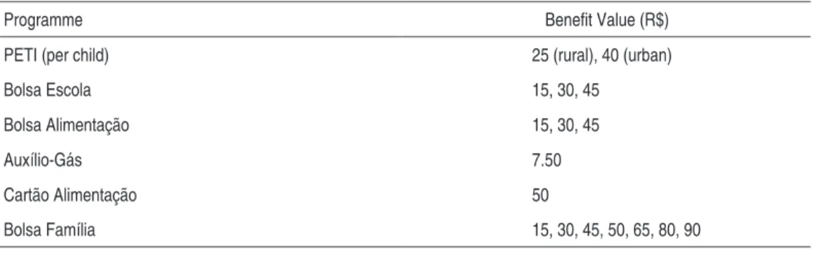
PNAD’s main questionnaire contains a set of questions in which the values of the different income sources a household may have are recorded. One of these questions refers to the value of household income that is obtained from both fi-nancial assets (e.g. interests and stock market shares) and transfers from social programmes. Note that income from both sources is reported together. However, one should expect that those households that derive income from financial assets tend not to receive benefits from social programmes. Based on this hypothesis, we use the information provided in this specific question to identify CCT benefi-ciaries. Specifically, our procedure makes use of the typical values of the benefits of CCT programmes to identify households that are (potentially) beneficiaries of these programmes. Table 2 presents the values typically transferred by each CCT
programme.3 Since a household may receive transfers from more than one of these
programmes, our procedure also uses the combination of these values to identify the beneficiary households. All values that were not equal to the typical values and
2 See Fuller (1987) for a general presentation of other methods to solve measurement error problems.
3 It should be noted that in practice we use the values of R\$7 or R\$8 to capture the Auxílio-Gás
their combinations were treated as income from financial assets or from non-CCT
programmes.4
Table 2 – Typical Values of Beneits Transferred by CCT Programme
Programme Beneit Value (R$)
PETI (per child) 25 (rural), 40 (urban)
Bolsa Escola 15, 30, 45
Bolsa Alimentação 15, 30, 45
Auxílio-Gás 7.50
Cartão Alimentação 50
Bolsa Família 15, 30, 45, 50, 65, 80, 90
Source: Barros et al. (2007, Table 6).
To validate our procedure, we take advantage of the fact that the 2004 version of PNAD included a special questionnaire that directly asked whether the household was participating in the Federal CCT programmes. Using the information provi-ded by this special questionnaire as a reference, we then check if our procedure is consistent. Specifically, we calculate the proportion of recipient and non-recipient individuals of CCT programmes according to the special questionnaire and to our procedure. The results are presented in Table 3.
Table 3 – Proportion of CCT Beneficiaries: Comparison between the Special Questionnaire and the Procedure of Typical Values – (%)
Special Questionnaire
Recipient Non-recipient
Recipient 18.4 2.2
Typical Values
Non-recipient 1.7 77.7
Source: Based on microdata from PNAD 2004.
There are four main results that can be extracted from Table 3. Firstly, around 96% (18.4+77.7) of individuals were identically classified by both criteria. Secondly, around 8% (1.7/(1.7+18.4)) of those individuals identified as recipients by the
cial questionnaire were not classified as such by our procedure. In other words, approximately 92% of recipients were correctly identified by our proposed pro-cedure. Thirdly, around 3% (2.2/(2.2+77.7)) of those classified as beneficiaries by our procedure were not identified by the special questionnaire. Finally, Table 3 also reveals that programme participation is only slightly overestimated by our procedure. Indeed, while our procedure classifies 20.6% (18.4+2.2) of the popu-lation as beneficiaries, this proportion is 20.1% (18.4+1.7) according to the special questionnaire.
Figures 1 and 2 present complementary evidence on the accuracy of our procedure. Still based on PNAD 2004, Figure 1 presents the proportion of individuals in each
percentile of the per capita family income distribution that are recipients of CCT
programmes. One of the curves in this Figure is based on our procedure, while
the other is calculated from the information of the special questionnaire.5 Apart
from revealing that the Brazilian CCT programmes were reasonably well targeted to the poor, Figure 1 evinces that our procedure seems to consistently classify the recipients of CCT programmes along almost the entire income distribution. As expected, our procedure tends to slightly overestimate programmes’ participation for richer individuals.
0 10 20 30 40 50 60
0 10 20 30 40 50 60 70 80 90 100
percentile of family per capita income distribution
percentage of individuals
Supplementary questionnaire Typical values
Source: Based on microdata from PNAD 2004.
Figure 1 – Percentage of CCT Beneficiaries across Percentiles of the Income Distribution: Special Questionnaire and Method of Typical Values
5 In order to smooth these curves, they are depicted as a moving average of ten percentiles. For example, the point corresponding to the 10th percentile represents the average of the 1st to the
As a final validation test of our procedure, we exploit two facts that are related to the historical evolution of CCT programmes in Brazil. The first is that all CCT
programmes but one (namely PETI) started operating after 2001 (see Table 2).
Hence, if our procedure is correct we should expect to detect fewer CCT indivi-duals before that year. The second fact is that the coverage of CCT programmes progressively increased since 2001, so our procedure should be capable to detect this movement as well. Figure 2, which is solely based on our procedure, presents
the evolution of the percentage of individuals along the per capita family income
distribution for a set of years since 1999.6,7 As it can be seen from this figure, the
two historical facts previously mentioned seem to be reasonably well captured by our proposed method: (1) the line corresponding to 1999 is almost flat; and (2) the lines corresponding to the years after 1999 are basically overlapped.
0 10 20 30 40 50
0 10 20 30 40 50 60 70 80 90 100
percentiles of the family per capita income distribution
percentage of individuals
1999 2001 2003 2005
Source: Based on microdata from PNAD.
Figure 2 – Percentage of CCT Beneficiaries across Percentiles of the Income Distribution: Method of Typical Values – Selected Years
Overall, we believe that the evidence presented in this subsection indicates that our proposed procedure is sufficiently accurate to measure CCT programme participa-tion over time. Thus, in our regression analysis, the variable that we use to measure
programme participation is based on this procedure. Specifically, in the regressions
we use the proportion of beneficiary individuals at the municipal level.8
3.2 Descriptive statistics
As the labour supply effects of CCT programmes may be different for males and fe-males, our empirical analysis is implemented separately by gender group. In addition, since the effects of interest may also vary across the different parts of the income distribution, results are obtained separately for the overall sample of each sex and for
the samples of males and females from families below the median per capita family
income of the municipality they live in (henceforth called below-median samples).9
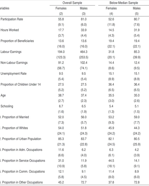
The sample mean and standard deviation of the variables used in our regression analysis are presented in Table 4. Columns (2) and (3) display these statistics for the overall samples of females and males respectively, while columns (4) and (5) contain the estimates respectively for the below-median samples of females and males. Statistics are presented for all years combined (2001-2005). Almost all estimates are calculated for individuals of each gender group above the age of 15 years. The exceptions are: (1) the proportion of children under 14 years old, for which there is no distinction between the sexes; (2) the proportion of beneficiaries of CCT programmes, which includes individuals of all ages and genders; and (3) the unemployment rate, which is calculated for individuals older than 15 years of both sexes together.
The first two rows of Table 4 display the estimates of the two response variables used in the regression analysis: the labour market participation rate (Row (1)) and the mean number of hours worked during the reference week of the survey (Row
(2)).10 On average, women have lower participation rates and work fewer hours
than men. This is observed for both the overall and the below-median samples. Also noticeable is that the participation rate and hours worked of poorer women tend to be smaller than those of the overall female sample. Interestingly, this is only observed for the number of hours worked in the case of males.
8 One may raise the question that we are also including recipient rich families in our measure of programme participation. Thus, we also calculated programme participation excluding all fami-lies that were below the average (over the years) 75th and 90th percentiles of the family per capita
income. At the municipal level, the correlation between our programme participation variable and the measure based on the 75th (90th) percentile is around 0,98 (0,99).
9 The reason for establishing the threshold at the median is that the sample size for some munici-palities is not very large.
Table 4 – Descriptive Statistics: Mean of Variables for All Years (2001-2005)
Overall Sample Below-Median Sample
Variables Females Males Females Males
(2) (3) (4) (5)
1. Participation Rate 55.8 81.0 52.6 80.7
(9.1) (6.0) (11.8) (7.6)
2. Hours Worked 17.7 33.9 14.5 31.9
(3.7) (4.4) (4.3) (5.4)
3. Proportion of Beneiciaries 13.6 13.6 19.4 19.4
(16.0) (16.0) (22.1) (22.1)
4. Labour Earnings 194.0 464.3 31.8 85.3
(123.3) (253.5) (20.1) (39.9)
5. Non-Labour Earnings 91.2 102.4 14.4 12.4
(56.7) (74.1) (8.6) (9.5)
6. Unemployment Rate 9.5 9.5 15.1 15.1
(5.4) (5.4) (8.9) (8.9)
7. Proportion of Children Under 14 27.5 27.5 36.4 36.4
(5.2) (5.2) (6.5) (6.5)
8. Age 38.7 37.4 35.5 35.0
(2.7) (2.3) (3.0) (2.6)
9. Schooling 6.7 6.5 5.4 5.1
(1.6) (1.9) (1.3) (1.5)
10. Proportion of Married 52.0 56.0 53.2 59.0
(7.3) (5.7) (9.3) (7.7)
11. Proportion of Whites 54.0 51.8 45.9 44.3
(24.1) (24.3) (24.2) (24.2)
12. Proportion of Urban Population 85.3 83.7 82.1 80.5
(21.3) (22.8) (24.5) (25.9)
13. Proportion in Adm. Occupations 11.6 6.2 6.3 4.2
(6.6) (4.0) (6.1) (3.9)
14. Proportion in Service Occupations 31.0 11.9 44.5 14.1
(10.9) (5.8) (18.1) (9.1)
15. Proportion in Comm. Occupations 12.1 9.1 11.4 8.9
(5.8) (4.5) (8.0) (6.0)
16. Proportion in Other Occupations 45.2 72.7 37.8 72.8
Row (3) displays the estimates for our variable of interest: the proportion of indivi-duals that received benefits of CCT programmes. These estimates are based on the procedure described in subsection 3.1. As it can be seen, on average, around 14% of the population in all years of our sample was beneficiaries of CCT programmes. This figure increases to around 19% of the population that live in families whose
per capita income falls below the median family per capita income of their respec-tive municipalities.
Rows (4) and (5) shows the estimates of mean labour and non-labour income
res-pectively11 Labour earnings of women is substantially lower, on average, than that
of men (ratio of around 0.43 for the overall sample, and approximately 0.38 for the below-median sample). Interestingly, this gap is not so high in terms of non-labour income. In fact, women in the below-median sample seem to get slightly more than men in this part of the distribution.
Row (6) shows that the unemployment rate of females is substantially higher than that of males for both samples we use. Also noticeable is that the incidence of unemployment is much higher for poorer males and females.
Rows (7) shows that children under 14 years old represent around 28% of the
overall population and approximately 36% of the population below the median per
capita income. Rows (8) and (9) show that women are slightly older and more edu-cated than men. This is observed for both types of samples we are working with. Row (10) indicates that a lower proportion of women are married as compared to men. This difference is due to the larger size of the female population. As shown in Row (11), the proportion of white females is higher than that of males for the
overall population, but this difference is smaller for those below median per capita
income. Row (12) shows that the proportion of women living in urban areas is hi-gher than that of men for both types of samples we are considering.
Rows (13) to (16) present the occupational composition for females and males. As it can be seen, the proportion of females in the first three categories (specially in
service occupations) is higher than that of males.12
11 The measure of non-labour income does not include the value of transfers of CCT programmes. It includes the values of all other types of transfers available in the survey questionnaire such as pensions, rents, private transfers, capital income and benefits received from non-CCT pro-grammes. These last two components correspond to all non-typical values (and their combina-tions) of our procedure to identify beneficiaries of CCT programmes (see subsection 3.1). 12 Due to a change in the occupational codes used in PNAD from 2002 on, we were only able to
4 Some Theoretical Considerations
We are interested in the effects of CCT programmes on the labour supply of adults. Though our estimation of these effects is based on aggregate data, labour supply models at the individual/family level can provide useful insights about our effects
of interest.13 In what follows, we use the reasoning of simple, static models of
la-bour supply at the micro level.
In a standard model of individual labour supply, the effect of programmes’ transfers constitutes a pure income effect: the extra income from programmes’ grants allo-ws individuals to afford more of all goods. According to theory, the income effect should increase the demand for all normal goods, including both consumption and leisure (assuming the latter is a normal good). Hence, if adults allocate their time only between work and leisure, the standard individual model predicts that the effect of CCT programmes is unambiguously negative on the labour supply of adults.
However, given that CCT programmes are targeted to household units and impose conditionalities that restrict the time use of (some of) its members, a labour su-pply model at the family level seems more appropriate than the individual model to enhance the understanding of our effects of interest. Indeed, in family models, the decisions on the supply of labour of each household member take into account the restrictions on and the inter-dependencies between the time allocation of all household members.
Because programme grants are conditioned on children’s school attendance, the family model would predict that the shadow price (or relative value) of school rises, whereas the relative value of all other activities declines (say, work and leisure). This should lead to an increase in time allocated to school and a decrease in time devoted to all other activities together. In principle, it is unclear what the new com-position of time dedicated these other activities will be (RAvALLION; WODON, 2000). For instance, it is possible that there is no change in child labour, so the increase in schooling time comes at the expense of a reduction in children’s leisure. However, if there is a decline in the time children spend working, then there will
be less available labour within the household.14 In that case, the relative price of
labour inside the household tends to rise, which should lead to an increase in the
13 The extensive theoretical literature on labour supply is fairly well developed for both the indi-vidual and family units of analysis. However, the literature on more aggregate levels (e.g. munici-palities, states, or countries) is scarce. See Killingsworth (1983) for a survey of first-generation models of labour supply, and Blundell and Macurdy (1999) for a review of more recent models. 14 Assuming that education and leisure are normal goods, the pure income effect from the
labour supply of adults. Thus, given that the income effect operates in the other direction, the total effect of CCT programmes on adult labour supply becomes
ambiguous.15
5 Methodology
We use various linear regression models to investigate the effect of CCT program-mes on adult labour supply. We use a time series of cross-sections of 806 Brazilian municipalities that are followed over five years. This panel of municipalities is constructed from microdata of the 2001-2005 versions of PNAD (see section 3).
The effect of interest is assessed on two different variables: the participation rate and number of hours worked. The response variables and the covariates are descri-bed in section 3. Results are obtained separately by gender group and for two types of samples: one in which all individuals of each sex are used to construct the sample means (overall sample), and another in which the sample means of the sexes are
calculated only for individuals below the median per capita family income of their
respective municipalities (below-median sample). It is important to point out that the use of sample means may create measurement error problems, an issue that is
tackled through the application of instrumental variables methods.16
Consider the following equation for municipality j=1,...,J at time period t=1,...,T:
yjt = α + pjtγ + x’1jtβ1 + x’2jβ2+ ηj + ujt (1)
where y represents the response variable, p measures the proportion of individuals who
are CCT beneiciaries, (x1,x2) are vectors of time-variant and time-invariant control
variables respectively, η denotes unobserved municipality-speciic effects, and u is a
mean zero disturbance term that is assumed to be uncorrelated across municipalities and time periods but whose variance may be clustered at the municipal level. The parameter
α is an intercept, γ is our parameter of interest, and (β1, β2) are conformable vectors of
parameters respectively associated with the control variables in (x1,x2).
15 It should be pointed out that CCT eligibility criteria could also affect labour supply decisions within the household. Indeed, for CCT programmes that include periodic checks on family in-come, it is possible that (some) adults choose to work less (or not to work at all) so as to meet the income eligibility criterion of programmes. Another point to be raised is that compliance with the programmes’ conditionalities may also affect the allocation of time within the family. For instance, complying with periodic clinic visits and school attendance of children may decrease the labour supply of some family members, especially women.
In total we estimate five different models. The first is simply pooled OLS. The second is the random effects model, which differs from pooled OLS in that it expli-citly recognises the presence of municipality-specific effects, but assumes that they are uncorrelated with all covariates. This last assumption is relaxed in the fixed
effect model, which is our third model.17 This model can be estimated through
va-rious methods, the most common of them being the within-groups transformation. Applied to equation 2 this transformation produces:
jt jt
jt
jt
p
x
u
y
~
~
~
~
1 1 '
β
+
+
γ
=
(2)
where the tilde notation denotes:
ω
jt=
ω
jt−
ω
, with 11
T jt t
T
ω
−ω
=
=
∑
. Notice thatall time-invariant elements of equation 1 are swept out by the within-groups
trans-formation, including the municipality-specific effects, ηj. In a small-T setting as
ours, the fixed effects estimator of γandβ1 is consistent as long as there is strict
exogeneity.18
Another common method used in the panel data literature is the first-differences
transformation. Denoting ∆ωjt = ωjt - ωjt-1, equation 1 can then be expressed in
first-differences as:
∆yjt = ∆pjtγ + ∆x’1jtβ1 + ∆ujt (3)
Note that because of the first difference transformation we loose one time period,
so now t=2,...,T. Note too that the first-difference transformation also sweeps out
all time-invariant elements of equation 1. Our fourth and fifth models are based on equation 3. The fourth model simply estimates that equation under the assump-tion that there is strict exogeneity (see footnote 18). The fifth model relaxes strict exogeneity, allowing for the presence of correlation between the error term and the
covariates.19 Within our context, this type of correlation (endogeneity) may arise
from two basic sources. The first has to do with measurement issues. As discussed in section 3, since we measure our variables (in particular the regression covariates) at the municipal level, error-in-variable problems are likely to be present in our setting. The second is not related to measurement issues, but to more substantial (economic) factors. For instance, if there are relevant omitted variables in equation 1, it is likely that the error term will be correlated with the included covariates.
17 We report the usual Hausman test to assess the appropriateness of the random effects specification.
18 That is: E[ujs | Zjt for all j, and for all s and t, where Zjt = (pjt, x1jt, x2j).
19 More formally, it assumes that for all j: E[ujs | Zjt] = 0 if s > t and E[ujs | Zjt] ≠ 0 if s≤t, where
Zjt= (pjt,x1jt,x2j). Note that this assumption allows for contemporaneous correlation between the
A typical approach to deal with the presence of endogeneity is the use of instru-mental variables. The main requirements for instruments to be valid are that they are correlated with the endogenous covariates and at the same time orthogonal to the error term in the equation. Hence, given our assumptions, valid instruments
for (∆pjt,∆x1jt) are (pj,t-2,…,pj1;x1j,t-2,…,x1j1). Note that the use of lagged instruments
at time period t-2 implies that the fifth model is estimated for t=3,...,T. Since T=5, our model is identified, so we can apply the Sargan/Hansen test of over-identifying restrictions. The estimation method of the fifth model is the so-called
two-step GMM, as proposed by Arellano and Bond (1991).20
All models we estimate include year dummies. The standard errors of the models’ coefficients are estimated through the usual sandwich-type robust/clustered (at
the municipal level) method.21 The municipal population summed over the years
that are used in the corresponding models weights regressions. F-tests for the joint significance of the models’ coefficients are reported in the tables containing the regression estimates.
6 Results
We first present results for the participation rate and then for hours worked. For each sex, overall sample results are followed by below-median sample results.
6.1 Participation rate
6.1.1 Females
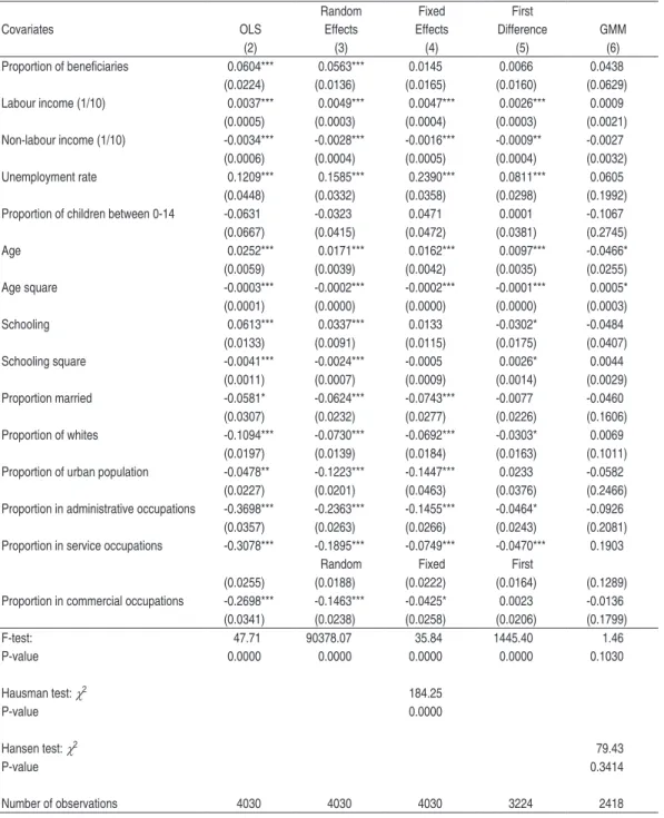
Regression results for the participation rate of all females are presented in Table 5. The coefficient of interest is the one corresponding to the variable proportion of beneficiaries. As this table shows, all point estimates of this coefficient are positive, though they are statistically significant only for the OLS and the random effects models. The Hausman test largely rejects the hypothesis that the random-effects specification is adequate. Indeed, as the following Tables will show, this hypothe-sis is strongly rejected by the Hausman test for both sexes, samples, and response variables we use. The Hansen test of over-identifying restrictions does not reject the null for the validity of the instruments used in the GMM model. This will also be observed in most of the following tables.
20 It has been found in the panel data literature that the standard errors of the two-step GMM may be inaccurately estimated in finite samples. To correct for that we apply the method put forward by Windmeijer (2005).
Table 5 – Efect of CCT Programmes on the Participation Rate of Females: Overall Sample
Random Fixed First
Covariates OLS Effects Effects Difference GMM
(2) (3) (4) (5) (6)
Proportion of beneiciaries 0.0604*** 0.0563*** 0.0145 0.0066 0.0438
(0.0224) (0.0136) (0.0165) (0.0160) (0.0629)
Labour income (1/10) 0.0037*** 0.0049*** 0.0047*** 0.0026*** 0.0009
(0.0005) (0.0003) (0.0004) (0.0003) (0.0021)
Non-labour income (1/10) -0.0034*** -0.0028*** -0.0016*** -0.0009** -0.0027
(0.0006) (0.0004) (0.0005) (0.0004) (0.0032)
Unemployment rate 0.1209*** 0.1585*** 0.2390*** 0.0811*** 0.0605
(0.0448) (0.0332) (0.0358) (0.0298) (0.1992)
Proportion of children between 0-14 -0.0631 -0.0323 0.0471 0.0001 -0.1067
(0.0667) (0.0415) (0.0472) (0.0381) (0.2745)
Age 0.0252*** 0.0171*** 0.0162*** 0.0097*** -0.0466*
(0.0059) (0.0039) (0.0042) (0.0035) (0.0255)
Age square -0.0003*** -0.0002*** -0.0002*** -0.0001*** 0.0005*
(0.0001) (0.0000) (0.0000) (0.0000) (0.0003)
Schooling 0.0613*** 0.0337*** 0.0133 -0.0302* -0.0484
(0.0133) (0.0091) (0.0115) (0.0175) (0.0407)
Schooling square -0.0041*** -0.0024*** -0.0005 0.0026* 0.0044
(0.0011) (0.0007) (0.0009) (0.0014) (0.0029)
Proportion married -0.0581* -0.0624*** -0.0743*** -0.0077 -0.0460
(0.0307) (0.0232) (0.0277) (0.0226) (0.1606)
Proportion of whites -0.1094*** -0.0730*** -0.0692*** -0.0303* 0.0069
(0.0197) (0.0139) (0.0184) (0.0163) (0.1011)
Proportion of urban population -0.0478** -0.1223*** -0.1447*** 0.0233 -0.0582
(0.0227) (0.0201) (0.0463) (0.0376) (0.2466)
Proportion in administrative occupations -0.3698*** -0.2363*** -0.1455*** -0.0464* -0.0926
(0.0357) (0.0263) (0.0266) (0.0243) (0.2081)
Proportion in service occupations -0.3078*** -0.1895*** -0.0749*** -0.0470*** 0.1903
Random Fixed First
(0.0255) (0.0188) (0.0222) (0.0164) (0.1289)
Proportion in commercial occupations -0.2698*** -0.1463*** -0.0425* 0.0023 -0.0136
(0.0341) (0.0238) (0.0258) (0.0206) (0.1799)
F-test: 47.71 90378.07 35.84 1445.40 1.46
P-value 0.0000 0.0000 0.0000 0.0000 0.1030
Hausman test: χ2 184.25
P-value 0.0000
Hansen test: χ2 79.43
P-value 0.3414
Number of observations 4030 4030 4030 3224 2418
To assess the magnitude of the effect of interest we can calculate its elasticity
at the mean values of (y,p) = (0.558,0.136). Taking the point estimates at face
value, their average equals approximately 0.04, which gives an elasticity of around 0.01. This implies that a 10% increase in the proportion of CCT beneficiaries would raise the female participation rate in 0.1%, which is a very small impact. Hence, we may conclude that the effect of the Brazilian CCT programmes on the female participation rate does not seem to be significant either in magnitude or on statistical grounds.
The effects of labour and non-labour income are respectively positive and nega-tive, and statistically significant across almost all models (the exception is the
GMM estimate22). These are the expected signs. Indeed, there is abundant
em-pirical evidence that shows that higher labour earnings affect positively the sup-ply of labour (see e.g. BLUNDELL; MACURDy, 1999). Also, higher non-labour earnings can be seen as a pure income effect, so we would expect a negative
impact of this variable on labour supply.23 Interestingly, higher unemployment
rates seem to increase the participation rate of women. This may be due to women’s decision to enter the labour force when their husbands become unem-ployed. Though not statistically significant, most estimates of the coefficient associated with the proportions of children in the municipality are negative. Hence, if anything, this may be indicating that children care activities inhibit women from participating in the labour market. Except for the GMM results, age seems to increase participation of women but at a decreasing rate. Similar results are observed for the schooling effect. Being married impacts negatively the labour force participation of females, a result that might be due to a lower necessity to work for married women.
A higher proportion of white females appears to be associated with lower parti-cipation rates. To the extent that labour supply decisions of black women may be affected by expectations of racial discrimination in the labour market, this result is unexpected. Some estimates of the effect of the proportion of females that live in urban areas are negative, whereas others are positive or statistically nil. In principle, the sign of this effect is ambiguous: on the one hand, urban areas tend to have more diversity in employment opportunities, which should lead to higher levels of labour force participation; on the other hand, rural individuals tend to help out in farm chores, a fact that should lead to lower participation levels in
22 Since instrumental variable estimation typically involves some loss of efficiency, it is not uncom-mon to lose statistical significance in this type of estimation.
rural areas. As for the occupational composition, most estimates indicate that higher shares of women in administrative, service, or commercial occupations tend to decrease female labour market participation (as compared to the excluded miscellaneous occupational category).
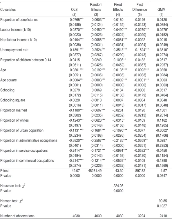
Table 6 reports the results for the participation rate of the below-median sample of females. Overall, the estimates of the effect of interest are quite similar to those obtained for the sample of all females. This is observed both in terms of the magnitude of the point estimates and in terms of statistical significance. Using the average of the point estimates (approximately 0.04), the elasticity of the effect of interest [calculated at the mean values of (y,p) = (0.526,0.194)] is around 0.01, implying that a 10% increase in the proportion of CCT
benefi-ciaries in Brazil would rise by 0.1% the participation rate of females whose per
Table 6 – Efect of CCT Programmes on the Participation Rate of Females: Below-Median Sample
' Random Fixed First
Covariates OLS Effects Effects Difference GMM
(2) (3) (4) (5) (6)
Proportion of beneiciaries 0.0765*** 0.0603*** 0.0160 0.0146 0.0120
(0.0186) (0.0124) (0.0134) (0.0123) (0.0654) Labour income (1/10) 0.0370*** 0.0450*** 0.0490*** 0.0270*** 0.0279*
(0.0023) (0.0023) (0.0024) (0.0020) (0.0152) Non-labour income (1/10) -0.0104*** -0.0088*** -0.0081*** -0.0022 0.0015
(0.0038) (0.0031) (0.0031) (0.0024) (0.0249) Unemployment rate 0.1891*** 0.2524*** 0.3513*** 0.1524*** 0.3810*
(0.0377) (0.0267) (0.0290) (0.0243) (0.2274) Proportion of children between 0-14 -0.0415 0.0249 0.1098** 0.0132 -0.2617
(0.0611) (0.0426) (0.0452) (0.0367) (0.2957) Age 0.0301*** 0.0192*** 0.0135*** 0.0092*** -0.0358
(0.0051) (0.0036) (0.0035) (0.0033) (0.0284) Age square -0.0004*** -0.0003*** -0.0002*** -0.0001*** 0.0003
(0.0001) (0.0000) (0.0000) (0.0000) (0.0003) Schooling 0.0279 0.0069 -0.0134 -0.0006 -0.0517 (0.0172) (0.0115) (0.0133) (0.0179) (0.0464)
Schooling square -0.0020 -0.0010 0.0007 -0.0004 0.0048
(0.0016) (0.0011) (0.0013) (0.0017) (0.0048) Proportion married -0.1180*** -0.0607*** -0.0261 0.0190 -0.1301 (0.0302) (0.0235) (0.0252) (0.0213) (0.2014) Proportion of whites -0.1243*** -0.0620*** -0.0315* -0.0109 0.1162
(0.0197) (0.0148) (0.0168) (0.0148) (0.1205) Proportion of urban population -0.1131*** -0.1684*** -0.1090*** -0.0077 -0.3002* (0.0234) (0.0198) (0.0295) (0.0254) (0.1706) Proportion in administrative occupations -0.3820*** -0.2567*** -0.2126*** -0.0659** 0.0287
(0.0401) (0.0314) (0.0300) (0.0261) (0.2953) Proportion in service occupations -0.2414*** -0.1721*** -0.0991*** -0.0532*** -0.0450 (0.0194) (0.0142) (0.0159) (0.0120) (0.1154) Proportion in commercial occupations -0.2147*** -0.1214*** -0.0526** -0.0109 -0.1398 (0.0274) (0.0226) (0.0232) (0.0181) (0.1569) F-test: 49.07 48281.49 43.30 897.82 1.57
P-value 0.0000 0.0000 0.0000 0.0000 0.0647
Hausman test: χ2 224.05
P-value 0.0000
Hansen test: χ2 90.85
P-value 0.1027
Number of observations 4030 4030 4030 3224 2418
Notes: See Table 5. The below-median sample refers to females who are below the median per capita
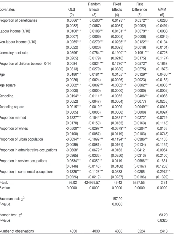
6.1.2 Males
Table 7 presents the results for the participation rate for the overall sample of males. All point estimates of the effect of interest are positive and, except for the GMM case, also statistically different from zero at conventional levels. Calculated for the average of the point estimates (approximately 0.03) and at
the mean values of (y,p) = (0.810,0.136), the implied elasticity here is around
0.005. This implies that a 10% increase in the proportion of CCT beneficiaries would raise the male participation rate by 0.05%. Though very small in mag-nitude, here we may conclude that the impact seems positive and statistically significant.
The effects of labour and non-labour income are respectively positive and nega-tive, though they seem to be smaller in absolute value than those obtained for all females. The unemployment rate seems to increase the participation rate of males, a result that has also been observed for women. In fact, the effects of the other covariates tend to be similar to what has been observed for the other gen-der group. The main exception is the variable proportion married, whose effect seems to be positive in the case of males. This may be due to the fact that males feel more compelled to be in the labour force when they are married.
Table 8 displays the results for the participation rate of the below-median sample of males. Estimates of the effect of interest are similar to those of the overall sample of males: all point estimates are positive and, except for the GMM, also statistically significant. Using again the average of the all point estimates (approximately 0.04)
and the mean values of (y,p) = (0.807,0.194), the elasticity is around 0.01, implying
Table 7 – Efect of CCT Programmes on the Participation Rate of Males: Overall Sample
Random Fixed First
Covariates OLS Effects Effects Difference GMM
(2) (3) (4) (5) (6)
Proportion of beneiciaries 0.0390*** 0.0391*** 0.0193** 0.0274*** 0.0146
(0.0104) (0.0076) (0.0090) (0.0102) (0.0515) Labour income (1/10) 0.0010*** 0.0008*** 0.0008*** 0.0006*** 0.0001
(0.0001) (0.0001) (0.0001) (0.0001) (0.0005) Non-labour income (1/10) -0.0022*** -0.0020*** -0.0012*** -0.0005** -0.0006 (0.0002) (0.0002) (0.0003) (0.0002) (0.0014) Unemployment rate -0.0398 0.0174 0.1368*** 0.0795*** 0.0451
(0.0264) (0.0212) (0.0232) (0.0213) (0.1457) Proportion of children between 0-14 -0.0312 0.0107 0.0952*** 0.0026 -0.2121
(0.0376) (0.0280) (0.0352) (0.0265) (0.1977) Age 0.0249*** 0.0253*** 0.0271*** 0.0143*** 0.0377**
(0.0031) (0.0024) (0.0028) (0.0021) (0.0152) Age square -0.0003*** -0.0003*** -0.0003*** -0.0002*** -0.0005*** (0.0000) (0.0000) (0.0000) (0.0000) (0.0002) Schooling -0.0037 -0.0027 -0.0012 0.0450*** -0.0324
(0.0044) (0.0041) (0.0062) (0.0101) (0.0234) Schooling square -0.0004 -0.0001 0.0006 -0.0035*** 0.0021
(0.0003) (0.0003) (0.0005) (0.0008) (0.0016) Proportion married 0.1404*** 0.0979*** 0.0381* 0.0373** 0.0591
(0.0213) (0.0172) (0.0196) (0.0174) (0.1351) Proportion of whites -0.0387*** -0.0158* -0.0360*** -0.0058 -0.0185 (0.0099) (0.0083) (0.0117) (0.0121) (0.0723) Proportion of urban population -0.0657*** -0.0945*** -0.1326*** -0.0242 -0.0623 (0.0097) (0.0089) (0.0222) (0.0204) (0.1672)
Random Fixed First
Proportion in administrative occupations -0.0731** -0.0462 -0.0163 0.0059 -0.0977 (0.0361) (0.0304) (0.0314) (0.0285) (0.1979) Proportion in service occupations -0.1128*** -0.0618*** 0.0155 -0.0798*** 0.3057*
(0.0208) (0.0185) (0.0199) (0.0213) (0.1622) Proportion in commercial occupations -0.1544*** -0.0987*** -0.0102 -0.0181 -0.2891* (0.0284) (0.0226) (0.0237) (0.0206) (0.1562) F-test: 114.15 569505.77 31.74 6905.91 1.85
P-value 0.0000 0.0000 0.0000 0.0000 0.0195
Hausman test: χ2 208.10
P-value 0.0000
Hansen test: χ2 52.77
P-value 0.9760
Number of observations 4030 4030 4030 3224 2418
Table 8 – Efect of CCT Programmes on the Participation Rate of Males: Below-Median Sample
Random Fixed First
Covariates OLS Effects Effects Difference GMM
(2) (3) (4) (5) (6)
Proportion of beneiciaries 0.0566*** 0.0503*** 0.0193** 0.0372*** 0.0280
(0.0082) (0.0067) (0.0081) (0.0092) (0.0491) Labour income (1/10) 0.0100*** 0.0108*** 0.0131*** 0.0079*** 0.0033
(0.0007) (0.0006) (0.0008) (0.0008) (0.0046) Non-labour income (1/10) -0.0265*** -0.0279*** -0.0236*** -0.0122*** -0.0134 (0.0022) (0.0023) (0.0023) (0.0018) (0.0101) Unemployment rate 0.0396* 0.0784*** 0.1990*** 0.1051*** 0.0726
(0.0205) (0.0179) (0.0216) (0.0175) (0.1174) Proportion of children between 0-14 0.0084 0.0824*** 0.1780*** 0.0572** 0.1658
(0.0313) (0.0279) (0.0330) (0.0275) (0.1878) Age 0.0180*** 0.0181*** 0.0155*** 0.0129*** 0.0430***
(0.0026) (0.0024) (0.0026) (0.0023) (0.0153) Age square -0.0002*** -0.0002*** -0.0002*** -0.0002*** -0.0005*** (0.0000) (0.0000) (0.0000) (0.0000) (0.0002) Schooling -0.0194*** -0.0111** -0.0055 0.0486*** -0.0086
(0.0052) (0.0047) (0.0064) (0.0077) (0.0255) Schooling square 0.0015*** 0.0010** 0.0009 -0.0049*** 0.0015
(0.0005) (0.0005) (0.0006) (0.0008) (0.0024) Proportion married 0.1327*** 0.1044*** 0.0831*** 0.0272* -0.0729
(0.0178) (0.0159) (0.0185) (0.0163) (0.1118) Proportion of whites -0.0500*** -0.0297*** -0.0379*** -0.0204** 0.0168
(0.0100) (0.0087) (0.0119) (0.0103) (0.0748) Proportion of urban population -0.0894*** -0.1099*** -0.1194*** -0.0386*** -0.1153 (0.0089) (0.0081) (0.0161) (0.0134) (0.1154) Proportion in administrative occupations -0.0668* -0.0672** -0.0163 -0.0412 -0.0054 (0.0365) (0.0336) (0.0350) (0.0313) (0.2100) Proportion in service occupations -0.0534*** -0.0359** 0.0119 -0.0586*** 0.1881
(0.0146) (0.0146) (0.0168) (0.0167) (0.1268) Proportion in commercial occupations -0.1326*** -0.1128*** -0.0333 -0.0265 -0.2972** (0.0226) (0.0219) (0.0237) (0.0186) (0.1399) F-test: 96.02 424969.57 49.42 5397.55 2.31
P-value 0.0000 0.0000 0.0000 0.0000 0.0020
Hausman test: χ2 157.90
P-value 0.0000
Hansen test: χ2 63.20
P-value 0.8325
Number of observations 4030 4030 4030 3224 2418
Notes: See Table 5. The below-median sample refers to males who are below the median per capita
Similar to the comparison between the two samples of females, here it is also no-ticeable that labour income, non-labour income, and the unemployment rate have higher impacts (in absolute value) than those observed for overall sample of males. The rest of the results are also similar between the two samples of males.
6.2 hours Worked
We now discuss the regression results for the case in which the response variable is the mean number of hours worked at the municipal level. It is important to recall that this variable has been measured including those individuals that worked zero hours (i.e. the unemployed and those out of the labour force). This implies that shifts in our measure of the mean number of hours worked are driven either by changes in the proportion of individuals with zero hours or by changes in the mean of strictly positive hours of work.
More formally, let h denote the individual labour supply of hours, π the proportion
of individuals with h=0, and µ* = E[h | h > 0] the mean of the distribution of
strictly positive hours. Then, the mean number of hours worked can be written as:
µ = E[h] = π. E[h | h=0] + (1-π) . E[h | h > 0] = (1-π).µ*. Thus, µ can be affected
either by changes in π or in µ*.
CCT programmes may directly affect both π and µ*.24 For example, π can vary
be-cause these programmes may make some of those who are out of the labour force
to find a job. Also, µ* can change because these programmes may directly affect
the supply decisions of hours of those already employed. Moreover, changes in π
can indirectly affect µ*. For instance, using the previous example, if the group of
newly employed individuals (i.e. those who moved from out of the labour force)
has average hours below (above) the initial µ*, then we should observe a decrease
(increase) in µ*.
It is not straightforward to connect the effects of CCT programmes on the supply of hours and the participation rate. First, there is an intrinsic relationship between
the proportion of individuals with zero hours of work and the participation rate.25
Since CCT programmes may trigger movements of individuals across the different labour market statuses (employment, unemployment, and inactivity), it is possible that: (1) the participation rate and proportion of zero-hours individuals change in
24 For simplicity we omit conditioning variables in the notation for π and µ*. It should be under-stood, however, that π = Pr[h=0 | p, X] and µ* = E[h | h>0, p, X], where p denotes programme participation and X represent a vector of control variables.
different directions; (2) one of them does not change at all; (3) they both change
in the same direction.26 Second, as discussed in the previous paragraph, the mean
of strictly positive hours (µ*) may be indirectly affected by changes in proportion
of individuals with zero hours of work. In this sense, since the participation rate and the proportion of zero-hours individuals are intertwined, this channel also contributes to make the link between total labour supply of hours (i.e. µ) and the participation rate less direct. In fact, in order to investigate empirically the con-nection between the effects of CCT programmes on these two variables, it seems necessary to develop a method that is capable of isolating the programmes' effects on the set of all relevant variables that affect the total labour supply of hours. This task is beyond the scope of this paper, though.
6.2.1 Females
Table 9 reports the results for the overall sample of females. As it can be seen from this Table, all point estimates of the effect of interest are negative, with three out of five being statistically significant. In terms of magnitude, if we take the average of all estimates (approximately -1.6), the elasticity [calculated at the mean values of (y,p) = (17.7,0.136)] is around -0.01. This implies that the impact of a 10% increase in the proportion of CCT beneficiaries would reduce in 0.1% the mean number of hours worked by females. Though negative, this appears to be a small impact.
It is interesting to note that the effects of the Brazilian CCT programmes on the mean number of hours worked and the participation rate of females seem to be different. Indeed, the evidence shows that the impact is approximately nil on the participation rate of women but negative on their supply of hours. As discussed before, since there are various different channels through which these two effects may be connected, it is difficult to offer an explanation for this result.
The signs of the effects of the other covariates are similar to those found for the participation rate. A noticeable exception is the unemployment rate, whose effect on hours is negative.
Table 9 – Efect of CCT Programmes on Hours Worked of Females: Overall Sample
Random Fixed First
Covariates OLS Effects Effects Difference GMM
(2) (3) (4) (5) (6)
Proportion of beneiciaries -1.4585** -1.0271*** -0.6524 -2.6266*** -2.3830 (0.6205) (0.3617) (0.5379) (0.6191) (2.0709) Labour income (1/10) 0.1961*** 0.2005*** 0.2194*** 0.1158*** 0.1068
(0.0210) (0.0088) (0.0170) (0.0136) (0.0793) Non-labour income (1/10) -0.1307*** -0.1075*** -0.0684*** -0.0400** -0.0207 (0.0202) (0.0141) (0.0184) (0.0166) (0.1163) Unemployment rate -18.5929*** -16.7559*** -15.2628*** -8.7690*** -16.2545** (1.5306) (0.9785) (1.0829) (1.1643) (8.0390) Proportion of children between 0-14 -2.8796 0.9053 2.1828 3.3829* -3.8405
(2.3694) (1.3244) (1.6180) (1.7691) (10.7241) Age 1.0411*** 0.8222*** 0.7663*** 0.4442*** -1.3847
(0.2005) (0.1229) (0.1464) (0.1384) (0.8700) Age square -0.0141*** -0.0109*** -0.0099*** -0.0054*** 0.0151
(0.0022) (0.0013) (0.0016) (0.0016) (0.0096) Schooling 3.0372*** 1.2467*** 0.1818 -4.4180*** -0.8848
(0.4223) (0.2603) (0.4361) (0.6282) (1.2524) Schooling square -0.2314*** -0.0860*** 0.0171 0.3738*** 0.0873
(0.0350) (0.0206) (0.0339) (0.0496) (0.0905) Proportion married -5.0810*** -4.9810*** -5.6113*** -2.9856*** -4.9769 (1.0301) (0.7787) (0.8706) (0.9573) (7.0995) Proportion of whites -0.6220 -0.9371** -1.3794** -1.1175** 0.1409 (0.5693) (0.4101) (0.5537) (0.5621) (3.9200) Proportion of urban population 0.5451 -1.7028*** -3.6178** 0.2405 6.3285
(0.8091) (0.5571) (1.4299) (1.4168) (9.3572) Proportion in administrative occupations -9.1480*** -3.8009*** -1.6881* -0.6317 -2.0769 (1.2446) (0.8515) (0.9729) (0.9999) (6.8999) Proportion in service occupations -5.8759*** -0.0395 2.6156*** 1.2695* 6.8951
(0.8517) (0.5300) (0.7103) (0.6481) (4.3442) Proportion in commercial occupations -3.8321*** 0.7889 2.4720*** 1.5014* 5.9166
(1.1287) (0.7430) (0.8385) (0.8376) (6.2977) F-test: 64.35 2042.76 50.46 959.02 2.10
P-value 0.0000 0.0000 0.0000 0.0000 0.0057
Hausman test: χ2 214.60
P-value 0.0000
Hansen test: χ2 68.62
P-value 0.6851
Number of observations 4030 4030 4030 3224 2418
Table 10 contains the results for the below-median sample of females. All point estimates of the effect of interest display a negative sign, but only one
of them is statistically significant at the 10% level.27 From the average of the
point estimates (approximately -0.47), the elasticity [calculated at the mean values of (y,p) = (14.5,0.194)] is close to -0.01, implying that a rise in 10% in the proportion of CCT beneficiaries would lead to a reduction in -0.1% in the mean number of hours worked by females below the their respective
munici-palities’ median per capita income. Once again, the impact is quite small. In
contrast to the case of all females, here the effect of interest does not seem to be statistically different from zero. Hence, for this sample, the effects on both the participation rate and the supply of hours are not significant either statistically or in magnitude.
In terms of sign, the effects of the other covariates are in line with those obtained for the overall sample of females. The magnitude of the effects asso-ciated with labour and non-labour income is higher (in absolute terms) for the below-median sample of females. The opposite applies for the unemployment rate.
Table 10 – Efect of CCT Programmes on Hours Worked of Females: Below-Median Sample
Covariates OLS Effects Effects Difference GMM
(2) (3) (4) (5) (6)
Proportion of beneiciaries -0.2359 -0.0932 -0.1971 -0.8286* -1.0153 (0.5610) (0.3043) (0.4015) (0.4226) (1.7312) Labour income (1/10) 1.7796*** 2.0554*** 2.2308*** 1.2844*** 1.3591***
(0.0907) (0.0511) (0.0930) (0.0860) (0.4421) Non-labour income (1/10) -0.6066*** -0.5466*** -0.4880*** -0.0318 -1.1543* (0.1355) (0.0864) (0.0972) (0.0964) (0.6048) Unemployment rate -11.6967*** -9.3645*** -7.9904*** -3.9574*** -14.2965*** (1.0357) (0.7218) (0.7478) (0.8010) (5.0715) Proportion of children between 0-14 0.9797 4.1298*** 5.3883*** 3.9187*** 2.2846
(1.9722) (1.1460) (1.4268) (1.3168) (2.2126) Age 1.0684*** 0.5867*** 0.4510*** 0.2745** 0.5995***
(0.1717) (0.1058) (0.1160) (0.1140) (0.1696) Age square -0.0127*** -0.0076*** -0.0060*** -0.0032** -0.0067*** (0.0019) (0.0012) (0.0013) (0.0013) (0.0024)
Random Fixed First
Schooling 1.9203*** 0.4189 0.0061 -1.3598** -0.4065
(0.5245) (0.2821) (0.4503) (0.5877) (0.6940) Schooling square -0.1969*** -0.0731*** -0.0317 0.1164** 0.0358
(0.0484) (0.0275) (0.0423) (0.0557) (0.0695) Proportion married -7.9715*** -4.4348*** -3.3059*** -0.3785 -6.7331*** (1.0388) (0.6575) (0.8067) (0.7410) (1.8405) Proportion of whites -1.2109** -0.3970 0.2897 -0.2827 -0.0106 (0.5789) (0.4033) (0.4789) (0.4838) (0.7250) Proportion of urban population -1.6817** -3.0585*** -1.3986 0.6730 -1.5359
(0.7914) (0.4893) (0.9756) (0.8464) (1.3863) Proportion in administrative occupations -9.7746*** -4.2795*** -2.5795*** 0.0624 1.9328
(1.2427) (0.9255) (0.9756) (0.9279) (1.5897) Proportion in service occupations -5.0698*** -1.2654*** 0.0039 0.2418 0.8091
(0.5741) (0.3762) (0.4425) (0.3984) (0.6367) Proportion in commercial occupations -4.8685*** -1.5492*** -0.4474 0.3100 1.5322
(0.8028) (0.6006) (0.6592) (0.6192) (1.0069) F-test: 82.58 2990.05 76.99 615.18 9.13
P-value 0.0000 0.0000 0.0000 0.0000 0.0000
Hausman test: χ2 188.41
P-value 0.0000
Hansen test: χ2 106.24
P-value 0.0686
Number of observations 4030 4030 4030 3224 2418
6.2.2 Males
Table 11 presents the results for hours worked for the overall sample of males. Apart from OLS, all other models’ estimates of the effect of interest are positive. However, only one estimate is statistically different from zero at conventional le-vels. Taking the average of all estimates (approximately 0.73), the elasticity
[com-puted at the mean values of (y,p) = (33.9,0.136)] is less than 0.01. This implies
that increases in the proportion of CCT beneficiaries in Brazil would have no (or negligible) effects on males’ mean supply of hours.
Contrasting the estimates for the participation rate and for the mean supply of hours, there is a distinction as compared to the female case. There the former effect is basically nil, while the latter is negative; here the former effect is positi-ve, while the latter is nil. Hence, in term of sign, it seems that the Brazilian CCT programmes do not change the labour supply of hours of males but increase their participation rate; in contrast they decrease the supply of hours of females without affecting their participation rate. In all cases, however, it should be pointed out that, if there are any effects at all, they are quite small in magnitude.
As in the case of all females, the signs of the effects of the other covariates are similar to those found for the participation rate. Again, a noticeable exception is the unemployment rate, whose effect on hours is negative.
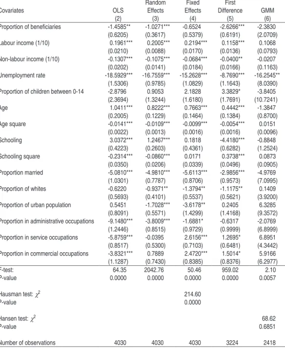
Table 12 displays the results for the below-median sample of males. All five point estimates of the effect of interest are positive, but only one is significant on statisti-cal grounds. The implied elasticity using the average of all estimates (approximately
1.43) and the mean values of (y,p) = (31.9,0.194) is around 0.01, implying that a
Table 11 – Efect of CCT Programmes on Hours Worked of Males: Overall Sample
Covariates OLS Effects Effects Difference GMM
(2) (3) (4) (5) (6)
Proportion of beneiciaries -0.6309 0.2766 0.5778 1.6025** 1.8281
(0.6899) (0.5126) (0.6402) (0.6381) (2.1012) Labour income (1/10) 0.0827*** 0.0611*** 0.0563*** 0.0473*** 0.0457
(0.0078) (0.0063) (0.0061) (0.0066) (0.0302) Non-labour income (1/10) -0.0932*** -0.0879*** -0.0481*** -0.0229 -0.0728 (0.0145) (0.0129) (0.0130) (0.0141) (0.0806) Unemployment rate -27.7628*** -24.5796*** -19.7568*** -9.7300*** -30.4398*** (1.6085) (1.2719) (1.3293) (1.4121) (7.7795) Proportion of children between 0-14 -1.6475 0.6947 4.9978** 0.3146 1.8819
(2.3585) (1.7397) (1.9476) (1.8773) (3.2170) Age 1.9424*** 1.7164*** 1.6313*** 0.7985*** 1.7843***
(0.1839) (0.1423) (0.1617) (0.1547) (0.2353) Age square -0.0246*** -0.0219*** -0.0208*** -0.0105*** -0.0217*** (0.0020) (0.0015) (0.0018) (0.0017) (0.0026) Schooling 0.9259** 0.4320 -0.6429* 2.4243*** -0.8057
(0.4092) (0.3101) (0.3641) (0.6685) (0.5156) Schooling square -0.1620*** -0.0817*** 0.0599** -0.2161*** 0.0826*
(0.0319) (0.0247) (0.0296) (0.0540) (0.0451) Proportion married 8.8246*** 7.6752*** 5.5037*** 3.4944*** 5.3435***
(1.4599) (1.1112) (1.2113) (1.1591) (1.7212) Proportion of whites -0.6144 -0.3354 -1.4747** 0.6491 1.2221
(0.6248) (0.5302) (0.6768) (0.7562) (0.9646) Proportion of urban population -2.6690*** -4.0697*** -5.3394*** 1.3547 -4.6355**
(0.6542) (0.6137) (1.3309) (1.4253) (1.8585) Proportion in administrative occupations -6.9284*** -5.1490*** -3.8760** -0.2570 -3.1583 (2.1265) (1.7767) (1.8579) (1.9048) (2.7311) Proportion in service occupations -3.1937** -1.3307 2.0506* -6.9829*** 0.0742
(1.2785) (1.0607) (1.1958) (1.4229) (1.7723) Proportion in commercial occupations -5.7593*** -2.8844** -0.4422 -0.4121 -1.3148 (1.6566) (1.3667) (1.3226) (1.3163) (2.0391) F-test: 119.35 194570.28 57.08 2059.64 19.27
Random Fixed First
P-value 0.0000 0.0000 0.0000 0.0000 0.0000
Hausman test: χ2 164.97
P-value 0.0000
Hansen test: χ2 93.74
P-value 0.2665
Number of observations 4030 4030 4030 3224 2418