$^{83\textrm{m}}$Kr calibration of the 2013 LUX dark matter search

83m

_{Kr calibration of the 2013 LUX dark matter search}

D.S. Akerib,1, 2, 3 _{S. Alsum,}4_{H.M. Ara´ujo,}5 _{X. Bai,}6_{A.J. Bailey,}5 _{J. Balajthy,}7 _{P. Beltrame,}8 _{E.P. Bernard,}9, 10 A. Bernstein,11 _{T.P. Biesiadzinski,}1, 2, 3 _{E.M. Boulton,}9, 10 _{P. Br´as,}12 _{D. Byram,}13, 14 _{S.B. Cahn,}10

M.C. Carmona-Benitez,15, 16 _{C. Chan,}17 _{A. Currie,}5 _{J.E. Cutter,}18 _{T.J.R. Davison,}8 _{A. Dobi,}19

E. Druszkiewicz,20 _{B.N. Edwards,}10 _{S.R. Fallon,}21 _{A. Fan,}2, 3 _{S. Fiorucci,}19, 17 _{R.J. Gaitskell,}17 _{J. Genovesi,}21 C. Ghag,22 _{M.G.D. Gilchriese,}19 _{C.R. Hall,}7 _{M. Hanhardt,}6, 14 _{S.J. Haselschwardt,}16 _{S.A. Hertel,}23, 19, 10, ∗

D.P. Hogan,9 _{M. Horn,}14, 9, 10_{D.Q. Huang,}17 _{C.M. Ignarra,}2, 3 _{R.G. Jacobsen,}9 _{W. Ji,}1, 2, 3_{K. Kamdin,}9 K. Kazkaz,11 _{D. Khaitan,}20 _{R. Knoche,}7 _{N.A. Larsen,}10 _{B.G. Lenardo,}18, 11 _{K.T. Lesko,}19 _{A. Lindote,}12 M.I. Lopes,12 _{A. Manalaysay,}18 _{R.L. Mannino,}24, 4 _{M.F. Marzioni,}8 _{D.N. McKinsey,}9, 19, 10_{D.-M. Mei,}13

J. Mock,21 _{M. Moongweluwan,}20 _{J.A. Morad,}18 _{A.St.J. Murphy,}8 _{C. Nehrkorn,}16 _{H.N. Nelson,}16

F. Neves,12 _{K. O’Sullivan,}9, 19, 10 _{K.C. Oliver-Mallory,}9 _{K.J. Palladino,}4, 2, 3 _{E.K. Pease,}9, 10 _{C. Rhyne,}17 S. Shaw,16, 22 _{T.A. Shutt,}1, 3 _{C. Silva,}12 _{M. Solmaz,}16 _{V.N. Solovov,}12 _{P. Sorensen,}19 _{T.J. Sumner,}5 M. Szydagis,21 _{D.J. Taylor,}14 _{W.C. Taylor,}17 _{B.P. Tennyson,}10 _{P.A. Terman,}24 _{D.R. Tiedt,}6 _{W.H. To,}25, 2, 3

M. Tripathi,18 _{L. Tvrznikova,}9, 10 _{S. Uvarov,}18 _{V. Velan,}9 _{J.R. Verbus,}17 _{R.C. Webb,}24 _{J.T. White,}24 T.J. Whitis,1, 2, 3 _{M.S. Witherell,}19 _{F.L.H. Wolfs,}20 _{J. Xu,}11 _{K. Yazdani,}5 _{S.K. Young,}21 _{and C. Zhang}13

(LUX Collaboration)

1_{Case Western Reserve University, Department of Physics, 10900 Euclid Ave, Cleveland, OH 44106, USA}

2

SLAC National Accelerator Laboratory, 2575 Sand Hill Road, Menlo Park, CA 94205, USA 3

Kavli Institute for Particle Astrophysics and Cosmology, Stanford University, 452 Lomita Mall, Stanford, CA 94309, USA

4

University of Wisconsin-Madison, Department of Physics, 1150 University Ave., Madison, WI 53706, USA

5_{Imperial College London, High Energy Physics, Blackett Laboratory, London SW7 2BZ, United Kingdom}

6_{South Dakota School of Mines and Technology, 501 East St Joseph St., Rapid City, SD 57701, USA}

7

University of Maryland, Department of Physics, College Park, MD 20742, USA

8_{SUPA, School of Physics and Astronomy, University of Edinburgh, Edinburgh EH9 3FD, United Kingdom}

9_{University of California Berkeley, Department of Physics, Berkeley, CA 94720, USA}

10

Yale University, Department of Physics, 217 Prospect St., New Haven, CT 06511, USA 11

Lawrence Livermore National Laboratory, 7000 East Ave., Livermore, CA 94551, USA

12_{LIP-Coimbra, Department of Physics, University of Coimbra, Rua Larga, 3004-516 Coimbra, Portugal}

13

University of South Dakota, Department of Physics, 414E Clark St., Vermillion, SD 57069, USA 14

South Dakota Science and Technology Authority, Sanford Underground Research Facility, Lead, SD 57754, USA

15

Pennsylvania State University, Department of Physics, 104 Davey Lab, University Park, PA 16802-6300, USA

16_{University of California Santa Barbara, Department of Physics, Santa Barbara, CA 93106, USA}

17

Brown University, Department of Physics, 182 Hope St., Providence, RI 02912, USA 18

University of California Davis, Department of Physics, One Shields Ave., Davis, CA 95616, USA

19_{Lawrence Berkeley National Laboratory, 1 Cyclotron Rd., Berkeley, CA 94720, USA}

20_{University of Rochester, Department of Physics and Astronomy, Rochester, NY 14627, USA}

21

University at Albany, State University of New York,

Department of Physics, 1400 Washington Ave., Albany, NY 12222, USA

22_{Department of Physics and Astronomy, University College London,}

Gower Street, London WC1E 6BT, United Kingdom 23

University of Massachusetts, Amherst Center for Fundamental Interactions and Department of Physics, Amherst, MA 01003-9337 USA 24

Texas A & M University, Department of Physics, College Station, TX 77843, USA 25

California State University Stanislaus, Department of Physics, 1 University Circle, Turlock, CA 95382, USA (Dated: August 9, 2017)

LUX was the first dark matter experiment to use a83mKr calibration source. In this paper we

describe the source preparation and injection. We also present several83m_{Kr calibration applications} in the context of the 2013 LUX exposure, including the measurement of temporal and spatial variation in scintillation and charge signal amplitudes, and several methods to understand the electric field within the time projection chamber.

∗_{[email protected]}

2

I. 83mKR AS A CALIBRATION SOURCE

The LUX experiment searches for galactic dark mat-ter particles scatmat-tering on target nuclei in a dual-phase xenon time projection chamber (TPC). Energy deposi-tions in the liquid Xe (LXe) produce observable signals via prompt scintillation (S1) and ionization charge, where liberated electrons drift upwards in an applied electric field and generate a delayed electroluminescence signal (S2) in the gaseous Xe (GXe). Light from both S1 and S2 is detected by photomultiplier tubes (PMTs) situated in two 61-PMT arrays above and below the 250 kg ac-tive xenon mass (see Ref. [1] for more details on detector design). The energy of an event may be inferred from the amplitude of its S1 and S2 signals. Additionally, and of vital importance in rejecting background events, the 3D position of an interaction may also be reconstructed. From the S2 signal, the distribution of photons in the top PMT array localizes the event in the xy-plane. The z position is calculated from the ionization electron drift time, i.e., the time interval separating the S1 and S2 sig-nals.

LUX has made extensive use of 83m_{Kr for calibration}

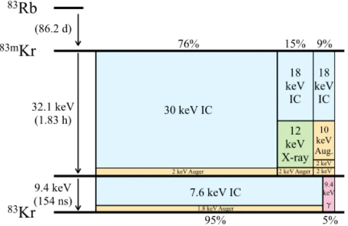
purposes. The decay of 83m_{Kr is illustrated in Figure 1.}

The parent isotope 83_{Rb is a practical source of} 83m_Kr

, due in part to its long half-life of 86.2 d. Once

pro-duced, the noble gas83m_{Kr may diffuse from the}

gener-ator material into the detector volume, decaying to83_Kr

with a half-life of 1.83 h, and releasing a total energy of 41.5 keV. The decay occurs in two transitions of 32.1 and 9.4 keV respectively, with an intervening half-life of 154 ns. These two transitions can each proceed according to multiple decay channels as indicated in Figure 1, but

in summary 83m_{Kr exhibits a high probability of}

inter-nal conversion (IC) followed by Auger emission, resulting in the high concentration of decay energy into electron modes. Two lower-probability modes of photon (gamma or x-ray) emission can occur, with a maximum photon energy of 12 keV.

The first uses of 83m_{Kr as a calibration source were}

in ALEPH [2] and DELPHI [3], with subsequent deploy-ments at STAR [4] and ALICE [5]. The IC and Auger electrons have served individually as electron energy cal-ibration lines in experiments measuring the tritium spec-trum at its endpoint (Mainz [6], Triotsk [7], KATRIN [8], Project 8 [9]). 83m_{Kr is a natural choice for calibrating} liquid noble-element dark matter direct detection exper-iments due to its inert nature and keV-scale decay en-ergy, similar to the energy scales sensed by these experi-ments. Initial demonstrations of83m_{Kr calibration in} liq-uid xenon, liqliq-uid argon, and liqliq-uid neon were performed

at Yale University [10–12]. The LXe response of 83m_Kr

has since been studied in detail, including [13] and [14]. It has been used as a calibration source for liquid argon detectors by the SCENE collaboration [15, 16], and to characterize a cryogenic distillation system [17].

In a liquid noble environment, the low-energy electrons and photons released by the decay deposit their energy

83m_Kr 32.1 keV (1.83 h) 9.4 keV (154 ns) 76% 15% 9% 5% 95% 30 keV IC 7.6 keV IC 18 keV IC 18 keV IC 12 keV X-ray 10 keV Aug. 9.4 keV 2 keV Auger 1.8 keV Auger 2 keV Auger 2 keV 2 keV 83_Kr 83_Rb (86.2 d) Decay Scheme

Somewhat novel presentation, copied from Carlos.

Keep meaning to compare these numbers between papers, make sure the literature is in consensus.

FIG. 1. Decay scheme of83mKr . The width of each column

is proportional to the branching fraction of that decay mode, the vertical divisions are proportional to energy partitioning among internal conversion electrons (blue), Auger electrons (yellow), x-rays (green), and gamma-rays (red). Numerical values from Reference [3].

within O(10 µm) of the decay vertex. These separations are much smaller than the spatial resolving power of the LUX detector (O(1 mm) [18]) or the typical electron dif-fusion distances during drift (also O(1 mm) [19]).

We describe here the first use of83m_{Kr to directly} cali-brate a dark matter experiment. This paper describes

the use of 83m_{Kr during the first (2013) exposure of}

the LUX experiment [20, 21]. The Darkside-50 [22] and XENON1T [23] collaborations have reported similar cal-ibrations.

II. 83mKR HARDWARE AND MIXING

Brookhaven National Laboratory produced the 83_Rb

for LUX, via proton irradiation of a nat_{RbCl target.}

Additional Rb radioisotopes can be produced, but with lower efficiency and shorter half-lives (86_{Rb 18.7d,}84_Rb

32.9d). The resulting 83_{Rb is stored in aqueous}

solu-tion for distribusolu-tion. After dilusolu-tion to reduce the spe-cific activity, a measured volume of the83_{Rb solution is} deposited on several grams of activated coconut carbon mediator (Calgon OVC 4x8). The carbon is baked at

∼100◦_{C for several hours under vacuum, to remove}

wa-ter and any other volatiles. This charcoal mediator was selected for its low radon emanation rate, previously mea-sured to be 9.4 mBq/kg [24]. Previous studies have found excellent binding of83_{Rb to charcoal mediators [11].}

The 83_{Rb-doped mediator is installed in the injection}

plumbing, as illustrated in Figure 2. To prevent the

spreading of possible charcoal particulates, the 83

Rb-doped mediator is contained between two sets of par-ticulate filtering, with pore size 15 µm and 0.5 µm. The

83m_{Kr generator plumbing straddles a pressure}

differen-tial in the main LUX gaseous Xe (GXe) circulation path. During injection this pressure differential motivates flow

3 Circulation Pump Mass Flow Controller to condenser from evaporator Getter Vacuum Pump 2 µ m 83_Rb 83m_{Kr Generator} 15 µ m 15 µ m 0.5 µ m 0.5 µ m

FIG. 2. Simplified plumbing and instrumentation diagram

showing the 83mKr generator (grey background) and its

set-ting for controlled injection. The injection path (red) starts at a high-pressure point on the main Xe circulation path (green) and ends at a low-pressure point near the main circulation pump inlet. A vacuum pump and its associated pump-out

line (blue) is used to evacuate the 83m_{Kr generator in some}

injection sequences. Valves with semicircle handles are auto-mated, all others are manual. Several particulate filters are noted, labeled by their pore diameter. Pressure gauges which play a role in the automated injection script are indicated by circles.

of GXe over the mediator and into circulation. The pres-sure differential is produced by the main GXe circulation

pump, and the rate of GXe flow through the83m_Kr

gen-erator is controlled using a mass flow controller down-stream from the mediator, with a typical control value of 0.50 slpm (much smaller than the flow of the main

circulation path). The83m_{Kr-doped GXe passes through}

a getter (SAES MonoTorr [25]) containing a 3 nm filter, further mitigating the risk of particulate contamination, or non-noble radioisotope contamination (including by

atomic83_{Rb ) of the detector volume.}

To release 83m_{Kr calibration doses of the desired}

ac-tivity and duration, the83m_{Kr injection system was}

op-erated in two modes, depending on the83_{Rb activity on}

the date of injection. For low-activity 83_{Rb, the valves}

along the injection flow path (red in Figure 2) were sim-ply opened for a duration proportional to the desired

83m_{Kr dose, typically several minutes. For high-activity}

83_{Rb, the}83m_{Kr generator volume was initially pumped}

to vacuum to eliminate the relic83m_{Kr activity prior to}

injection. In this mode, the injected activity resulted

only from 83_{Rb decays that occur during the injection}

time window (again an easily-controlled timescale, on the order of minutes).

Calibrations using83m_{Kr were performed on a regular}

(typically weekly) schedule throughout the data-taking campaign. An example of precise regular dosing is shown in Figure 3. A typical activity of ∼10 Bq was optimal for the measurement of electron lifetime in of LXe (see Sec-tion V), but depending on the specific calibraSec-tion goal, both higher- (∼100 Bq) and lower-rate injections were also performed. Hardware interlocks on pressure and flow readings would abort the injection in the event of unusual readings.

The flow and mixing of LXe within the LUX

time-Rate in each acquisition of Kr83m selection in S1 and S2, showing a date range with several (successful) dosings.

In grey are times omitted from the plot (either dead or other calibration) Uncertainties updated (dec13) to use exact poisson-described 1sigma. Arrows indicate bins of zero count.

01 02 03 04 05 06 07 08 09 10 11 12 13 14 Day of July 2013 10-5 10-4 10-3 10-2 10-1 100 rate [Bq] R ate [Bq ] Day of July 2013

FIG. 3. The 83mKr rate within a fiducial volume selection

over a period of two weeks, during which four injections were performed. The dosing system is able to inject a small and repeatable activity. For small injections, it takes ∼1 day for the 83m_{Kr activity to fall below the baseline electron recoil} background rate for that energy.

0 50 100 150 200 250 300 Drift Time [ 7 s] t₀ + 0.5 to 1.5 minutes t₀ + 1.5 to 2.5 minutes -20 -10 0 10 20

Radially Corrected S2 Position [cm] 0 50 100 150 200 250 300 Drift Time [ 7 s] t 0 + 2.5 to 3.5 minutes -20 -10 0 10 20

Radially Corrected S2 Position [cm] t

0 + 15 to 45 minutes

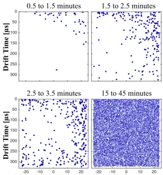
Mixing 1: showing convective cell rotating on minutes timescale, and also showing late-time uniformity

D ri ft T ime [ µ s] S2 Position (corr.) [cm] D ri ft T ime [ µ s] S2 Position (corr.) [cm] 0.5 to 1.5 minutes 1.5 to 2.5 minutes 2.5 to 3.5 minutes 15 to 45 minutes

FIG. 4. Reconstructed83mKr vertex positions are illustrated

within a thin slice of the LUX TPC for four distinct time

windows after a 83mKr injection. The x-axis is the S2 xy

position and the y-axis the electron drift time as measured by the time delay between S1 and S2 (the liquid surface is at zero drift time). The x-axis has here been rotated 45 degrees with respect to the typical LUX convention to better align with the dodecagonal shape of the TPC and the observed LXe flow axis. We use here the ‘corrected’ xy coordinates as described in SectionIV. A large-scale flow (clockwise in these coordinates) is observed, along with turbulent mixing.

projection chamber (TPC) can be observed using the 83m_{Kr injections, as illustrated in Figures 4 and 5.} Start-ing 60 seconds after GXe flow was initiated over the83

Rb-4 101 102 83m Kr Rate [Bq] 0 2000 4000 6000 8000 10000 12000 14000

Time Since Injection Start [s]

0 0.25 0.5 0.75

Fraction of Total Rate

Mixing 2: showing timescale of arrival and timescale of mixing

grey vertical bar is time window of Kr83m generator flow-through. lower panel shows fractional rate in equal fourths in drift time (red is top)

Time Since Injection Start [s]

83m

K

r R

ate

F

rac

ti

on

K

r R

ate

[Bq

]

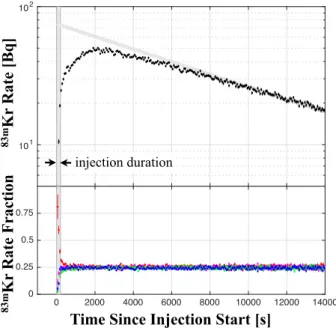
FIG. 5. TOP: The rate of83m_{Kr decays within the fiducial}

volume is shown as a function of time since the injection start

for a typical high-rate injection. The injection time (time

during which GXe is flowing over the 83_{Rb parent) is}

indi-cated by a gray band, in this case lasting several minutes.

An exponential decay expressing the83mKr decay half-life of

1.83h is highlighted in gray. BOTTOM: 83m_{Kr decays are}

here selected by drift time into four approximately equal vol-umes (red indicating the top fourth), and the relative fraction of83mKr activity in each fourth (R1/4/Rtot) is plotted. The

strong LXe mixing produces a homogeneous 83mKr activity

only minutes after injection, despite the gradual arrival of

83m_{Kr over one hour.}

doped mediator, the first83m_{Kr decays are seen near the}

liquid surface. A LXe flow (likely convective in origin) circulates this83m_{Kr-doped liquid with a velocity of a few} cm/s, completing a circuit from top to bottom and back over ∼2 minutes. As seen in the last panel of Figure 4 and

the lower panel of Figure 5, 83m_{Kr activity is uniformly}

distributed after several minutes. We assume the activity

is spatially homogeneous once the 83m_{Kr distribution is}

observed to be constant. The LXe flow pattern observed

with83m_{Kr was consistent with similar flow observations}

using222_Rn-218_{Po delayed α-particle coincidences [26].} As shown in the upper panel of Figure 5, a low rate of

83m_{Kr continues to enter the detector one hour after the}

injection sequence. This is attributed to 83m_{Kr activity}

slowly diffusing out the long and narrow GXe volume between the circulation path and the last outlet valve of the83m_{Kr injection line.}

S1 and S2 pulse amplitudes for 83m_{Kr decays lie}

out-side the typical dark matter search window. Further,

the presence of 83m_{Kr activity was seen to not increase}

the rate of low-energy triggers passing selection criteria

applied as in [21]. While it appears then that 83m_Kr

activity does not necessarily disqualify data from a low-energy low-background search, the short half-life allows

the conservative exclusion of this data with no significant decrease in search exposure.

In the following sections, we describe the use of83m_Kr for several calibrations central to the 2013 dark matter search of LUX, a search summarized in references [20] and [21].

III. STUDIES OF THE ELECTRIC FIELD

The 3D position reconstruction of ionization vertices requires an understanding of the path electrons take from their production site to their point of detection. In LUX, the latter occurs in close proximity to the liquid surface, where the observed S2 signal is generated via electrolu-minescence in GXe at high field. The distribution of S2 light sensed by the top PMT array is converted into an S2 position (xS2, yS2) using algorithms described in [18]. While the electric field is largely perpendicular to the liq-uid surface at all positions, the electric field lines in the first LUX science run (WS2013) include a small but non-zero radial component, inducing a radially-inward elec-tron drift. This radial field component is due to the

non-zero electrostatic transparency of the field cage. 83m_Kr

calibrations fill the TPC to its edges with a uniform spe-cific activity (activity per unit LXe volume), allowing for a robust consistency check of the observed drift field with that expected from geometrical effects alone.

A 3D model of the LUX geometry is constructed in

COMSOL Multiphysics R _{[27]. A 2D cross-section of}

this model is shown in Figure 6. Due to the

detec-tor’s geometrical complexity (relevant dimensions span 4 orders of magnitude), several model simplifications are adopted, each of which has been checked to ensure the simplification is of negligible effect to the resulting drift field. Details of boundaries within the ultra-high-molecular-weight polyethylene (UHMWPE) and polyte-trafluoroethylene (PTFE) volumes are omitted, includ-ing the weir, cathode cable and the heat exchanger. The anode grid and the bottom photomultiplier tube (PMT) shield grid are both modeled not as wires but as planes (the anode grid wires are of sub-mm spacing, and the bottom shield grid is backed by PMT faces of similar volt-age). The cathode and gate grids are accurately modeled as parallel wires of appropriate spacing, thereby account-ing for the electrostatic transparency of the real detector grids. These cathode and gate grids are simplified only in that the wire diameter is reduced to zero (from 206 and 101.6 µm respectively). Test models were studied to ensure this wire diameter change had negligible effect on the resulting solution, as expected from COMSOL’s use of the weak formulation [28] in solving the relevant partial differential equations.

The TPC diameter as measured between parallel oppo-site faces is 47.3 cm. The grid geometry is shown in Ta-ble I. Dielectric constants are included as LXe 1.95, GXe 1.0, PTFE 2.1, UHMWPE 2.3. Applied grid voltages are assigned as relevant to WS2013 operations; voltages

5

TPC geometry for electric field modeling (minimal labeling, descriptions will be verbose)

GXe LXe Anode Grid Gate Grid Cathode Grid PMT Shield Grid P TF E U H M WP E

FIG. 6. LEFT: Illustration of key features of the 3D LUX model, labeling materials and grids. The model is bounded by a the inner radius of the cryostat inner vessel at 31 cm. The central volume of LXe is bounded by 12 PTFE panels each of width 12.7 cm, forming a dodecagon of 23.7 cm apothem

(radius of inscribed circle). As described in the text, the

anode and bottom PMT shield grids are modeled as solid planes (making inclusion of detailed model geometry above the anode and below the bottom PMT shield unnecessary). RIGHT: A 3D map of electric field is obtained after the model in COMSOL is built, meshed and solved. Note the dodeca-hedral symmetry of the model in the relevant region.

of the field-shaping (dodecagonal) rings between cathode and gate follow expectation given the resistor within the voltage dividing chain.

TABLE I. Grid properties and voltages as relevant to the construction of the electric field model, including description of geometric simplifications.

Grid z† Wire_{Pitch Angle Modeled} HV

[cm] [µm] [mm] [deg] as [kV]

Top shield 58.6 50.8 5.00 135 Absent −1.0

Anode 54.9 28.4 0.25 N/A Plane 3.5

Gate 53.9 101.6 5.00 15 0 wires −1.5

Cathode 5.6 206.0 5.00 75 0 wires −10.0

Bottom shield 2.0 206.0 10.00 15 Plane −2.0

†

z is defined as vertical distance from the face of the bot-tom PMT array, accounting for thermal contraction as appropriate.

After solving for the electric field, field lines are used to simulate a uniform-activity dataset. Electron-like test particles follow the field lines to the liquid surface. The simulated electron drift velocity in LXe varies with

elec-0 5 10 15 20 25 rS2 [cm] 0 50 100 150 200 250 300 350 z S2 (dri ft ti m e) [ µ s] 0 5 10 15 20 25 r [cm] 5 10 15 20 25 30 35 50 45 40 z [c m ]

Result of field model, including comparison with Kr83m distribution added the electron path and the light grey shading

red/blue contours now at 50% density, matching run4 field modeling paper draft (blue is data, red is simulation)

dt vs r^2 with 71x71 bins.

bulk region is defined as 105<dt<238 and r<20 (we need to take 50% of some generic value)

-8 kV -6 kV -4 kV -2 kV rS2 [cm] D ri ft T ime [ µ s] r [cm] z [c m] e -rS2 0 5 10 15 20 25 rS2[cm] 0 50 100 150 200 250 300 350 Drift time t [µ s]

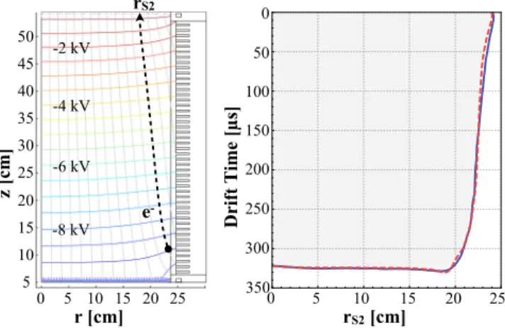
FIG. 7. LEFT: A simplified 2D COMSOL Multiphysics model (for illustration only) shows electric field lines and equipo-tentials in the LUX detector under WS2013 conditions. A radially-inward component is seen, resulting from the geome-try of the field cage and the grids. RIGHT: a uniform distri-bution of electrons is drifted in the electric field model, and the edge of their resulting distribution in tS2and rS2is plot-ted here in solid blue. A similarly defined edge can be drawn

from the 83mKr data (dashed red), and the simulation and

data can be seen to be consistent. The edge is defined as event density contours, specifically as the contour at which the event density in {rS22, tS2} falls to 50% of the average bulk value.

tric field as in Ref. [29]. The simulated drift time (tS2) and xy location of S2 light production (xS2, yS2) can be

compared with real 83m_{Kr data. A simple 2D version}

of this 3D comparison space is illustrated in the right panel of Figure 7. We find excellent agreement between simulation and data. It should be emphasized that no aspects of the field model are tuned to improve the level of agreement with data.

The slight curve seen in the reconstructed (S2) coor-dinates can be understood through inspection of the left panel of Figure 7. This panel shows equipotentials and field lines from the simpler 2D (axially symmetric) model

built for visualization purposes. When a 83m_{Kr decay}

occurs at high radius just above the cathode plane, the liberated electrons follow the field lines shown and escape the liquid at a radius reduced by several cm compared to the interaction radius. The radial field component traces its origin primarily to the electrostatic transparency of the cathode and gate grids (both of 5.0 mm pitch). This effect is strongest at high radii, producing a region of slightly reduced field above the cathode grid (created by upward leakage of the strong reverse-field region below the cathode) and a region of slightly enhanced field be-low the gate grid (created by downward leakage of the much higher above-gate field).

6 radial correction of raw S2 positions

In lower left, green is outside range of correction

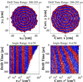
rS22 [cm2] Corr. r2 [cm2] D ri ft T ime [ µ s] yS2 [c m] xS2 [cm] Corr. x [cm] C or r. y [c m] Angle Range: 0-π/50 Angle Range: 0-π/50

Drift Time Range: 200-203 µs Drift Time Range: 200-203 µs

D ri ft T ime [ µ s]

FIG. 8. An illustration of the effect of the radial position

mapping between rS2 (left panels) and the resulting estimate

of the true event radius (right panels). The top panels show a thin slice of drift time, the bottom panels show a thin slice in angle. In all panels, the same concentric selections in rS2 are highlighted (red and blue) to make the mapping visible. Note that the mapping is only defined between 4 and 320 µs (events external to this range are green on the left, and not included on the right). Note also that the use of squared radius in the lower panels exaggerates the scale of the effect.

IV. MAPPING S2 RADIUS TO VERTEX

RADIUS

The field model could be employed as a mapping relat-ing the observed S2 position and the true event vertex po-sition, as {rvertex, φvertex, zvertex} = f ({rS2, φS2, tS2}). However, we find that in the WS2013 field configuration, only the radial component of position required the con-struction of a detailed mapping function. The radial cor-rection can be performed more precisely using the data alone, without relying on the accuracy of the field model and the electron drift simulation. A data-driven method is possible and advantageous in WS2013 due to the small scale of the corrections, with the added benefit that it allows for the correction of all radial effects, including small-scale field inhomogeneities and systematic errors in the {xS2, yS2} reconstruction algorithm.

The construction of a radius correction map relies on

the uniform density of the83m_{Kr calibration events. To}

ensure this uniform vertex density in real space, only data sufficiently long after activity injection (&2 h) is

employed in the map construction. 83m_{Kr events are}

grouped by vertex position into 11,520 wedge-shaped

po-sition selections: A tS2 range of 4 to 320 µs is divided

into 32 tS2 sections and 360 φS2 sections. These wedge

selections of 83m_{Kr events are not mutually exclusive,}

02 102 152 202 252

r2 [cm2]

normalized counts (arb.)

radial correction of raw S2 positions again, histogram in r^2 showing both before and after correction

(solid black is ideal dodecagon)

r

_[cm

_]

N

or

mal

iz

ed

C

ou

n

ts

[ar

b

.]

note: after a little digging, we realize claudio used older LRFs when defining these the radial correction map. with these older LRFs, the post-correction histogram is much flatter.

older LRFs

LRFs we actually used in publications

FIG. 9. The overall flattening effect of the radial position cor-rection is illustrated. A drift time selection is applied

match-ing the WS2013 analysis. Three histograms in r2 _{are shown:}

the rS22of a large sample of83mKr events (blue), the r2 distri-bution of those same83m_{Kr events after the radial correction} procedure (red), and the distribution of events uniform in a

dodecagonal prism in a toy Monte Carlo (black). The83mKr

sample shown in the blue and red histograms of this plot com-bine a wide range of dates through WS2013 running. The {xS2, yS2} reconstruction algorithm used here differs slightly from that used in the published analyses.

overlapping to the midpoint of neighboring selections in

both tS2 and φS2. Within a given wedge selection, the

rS2 distribution of 83mKr events is then ‘flattened’ by

shifting rS2 values such that they are of equal spacing

in r2 _{(with maximum radius matching the appropriate}

dodecagonal radius at that φ). Once each wedge

selec-tion region has received this treatment, the83m_{Kr event}

positions before and after the equal-spacing treatment are employed as a 3D linear interpolation mapping, as rvertex = f ({rS2, φS2, tS2}). The application of this interpolative mapping function is illustrated in Figures 8 and 9.

Given that variation in the drift field over time will affect the position mapping function, temporal varia-tion in the electric field is searched for using through

Kolmogorov-Smirnov comparisons of83m_{Kr distributions}

on widely separated dates within the WS2013 and found to be consistent with no change. This allows the con-struction of a single WS2013 interpolative mapping

func-tion from a single large83m_{Kr injection from May 2013,}

supplying 1.5 × 106_selected83m_{Kr events.}

V. THE POSITION-DEPENDENT

CORRECTION OF S1 AND S2 AMPLITUDES Detector efficiencies and gains may vary with position and time, requiring the construction of scintillation (S1)

7

and ionization (S2) signal amplitude corrections. 83m_Kr

events serve the role of ‘standard candles’ to produce monoenergetic signals of uniform initial scintillation and ionization amplitudes, before efficiency and gain effects. The S1 and S2 cases receive somewhat distinct treat-ments, described below.

In the S1 case, detector efficiency variation is the re-sult of a spatially-varying probability for a scintillation photon to strike a PMT window. To map this efficiency,

83m_{Kr data is binned in the 3D space of {x}

S2, yS2, tS2}.

An average 83m_{Kr S1 amplitude is found for each bin,}

and a 3D S1 correction map is constructed as the inverse

of these83m_{Kr S1 amplitudes, normalized to the S1}

am-plitude at the detector center: {0 cm, 0 cm, 159 µs}. The efficiency-correction map is then applied as a lin-ear interpolation on the 3D grid. Bin spacing of the

83m_{Kr dataset was chosen such that each bin received}

∼300 83m_{Kr events. It is observed that S1 correction}

maps vary negligibly with date, so a single large 83m_Kr

injection provided the S1 correction map, subsequently applied to the full range of WS2013 data.

The S2 case is more complex. A largely z-oriented efficiency variation dominates S2 variation, and results from electron capture on electronegative impurities dur-ing drift. Durdur-ing stable operation, the concentration of these impurities varies on a ∼week timescale. An inde-pendent S2 amplitude variation, oriented purely in the xy plane, results from three processes: the efficiency of electron extraction across the liquid-gas boundary, and the efficiency of producing and then observing electro-luminescence photons in the high-field gas region. The extraction efficiency and electroluminescence yield can vary dependent on detector conditions such as pressure, liquid level (dependent on circulation flow rate), detector tilt, and electrostatic grid deflection.

Two S2 correction maps are constructed, one for the z-dependent variation and one for the xy-dependent vari-ation, and these maps are applied independently. The z-dependent S2 correction consists of a simple exponential function of tS2, normalized to unity at the liquid surface (where electron lifetime has no effect on signal). The single-valued z correction is interpolated smoothly

be-tween measurements on83m_{Kr injection dates. It can be}

seen in Figure 10 that while the exponential description of the z-dependent S2 correction describes the data well in the fiducial volume, it is an imperfect description at the extrema of the drift path, where the drift field devi-ates from its nearly constant bulk value. This behavior at the extrema is consistent with impurities for which elec-tron capture cross section decreases with field, a category including O2 [30].

The S2 correction xy map is constructed by binning

83m_{Kr data in an xy grid and finding average S2}

ampli-tudes for each 2D bin. The xy map is applied as a 2D linear interpolation of the inverse S2 amplitudes, normal-ized to {x=0, y=0}. The xy grid spacing was variable

depending on83m_{Kr data sample size, binned such that}

each grid point represented ∼300 83m_{Kr events.}

Tem-poral variation between consecutive xy correction maps was much smaller than the z correction variation; the xy correction uses the nearest-in-time correction map.

83m_{Kr was injected weekly, a timescale set by}

varia-tion in electron lifetime. 222_{Rn decays (a constant,} low-level background) supply independent verification of the electron lifetimes, and verification that the weekly83m_Kr

schedule was sufficiently finely-spaced. Each83m_Kr

in-jection produces a typical sample size of ∼ 105 83m_Kr

decays. In the event of a sudden LXe purity change (such as a short circulation outage), data between the

most recent83m_{Kr injection and the purity drop event}

are corrected assuming the last S2 correction map before purity change. Data taken between a purity change and

the first subsequent83m_{Kr are discarded.}

As shown in Figure 1, 83m_{Kr decay proceeds through}

two transitions, separated by a 154 ns half-life. Because the S2 signals are of 1.0–1.9 µs FWHM (depending on z position), the two decay steps are merged in the S2 signal. On the other hand, the S1 pulse width is short (∼100 ns after filtering) such that a significant fraction

of 83m_{Kr decays exhibit separation into two S1 pulses,}

which we refer to by their ordering as S1a and S1b (32.1 and 9.4 keV, respectively). It has been observed in [31] that the S1b amplitude (and by implication the S1a+S1b summed amplitude) varies depending on the intervening time delay. A short delay enhances electron-ion recombi-nation in the second decay (S1b), increasing the resulting scintillation and thus boosting the S1b amplitude. Be-cause the S1a+S1b amplitude depends on the stochastic

decay time between the two transitions, use of83m_{Kr S1}

amplitude as a standard candle for calibration is only possible if one specifies and adheres to a consistent delay range at all positions. Conversely, if a consistent delay range is used, the complexity of time delay amplitude variation can be ignored. In the LUX WS2013 case, the summed S1 area is employed for S1 area corrections, and the transition time separation range is specified as 0 to 1200 ns. These choices maximize useful calibration statis-tics. S1 amplitudes in the separate S1a and S1b cases can be used as a cross check, as in the lower panels of Fig-ure 11.

The resolution and central value of the S1 and S2 peaks can be used to monitor the efficacy of amplitude correc-tion maps. The resolucorrec-tion, σ/µ, is calculated from Gaus-sian fits to the S1 and S2 amplitude distributions. For

fiducial volume events in the largest83m_{Kr dataset (May}

2013), the relative resolution of the combined 41.5 keV peak improves from 12.3% to 8.1% in S1 and from 19.3% to 15.3% in S2 after these corrections (see Figure 11). This S1 resolution improvement is typical of every data set, due to the stability of the position-dependent effects (e.g., photon mean free path, material surface reflectivi-ties). On the other hand, the S2 improvement is highly dependent on the electron lifetime. For the largest83m_Kr dataset, the lifetime is 750 µs, typical of WS2013 (which exhibits a range of lifetimes of 600–950 µs). We also look at the stability of83m_{Kr S1 and S2 central values over the}

8

Relative scales of Kr83m, as recorded for correction

red circle indicates the normalization points (center for S1, top center for S2)

D ri ft T ime [ µ s] yS2 [c m] Drift Time [µs] Relative Amplitude yS2 [cm] xS2 [cm] xS2 [cm] S1 Relative to [0cm, 0cm, 159µs] S2 Relative to [0cm, 0cm, 0µs] R el . A mp li tu d e Res.

FIG. 10. Maps of relative 83m_{Kr S1 and S2 amplitudes, as}

derived for an example date of May 10, 2013. The 3D map of S1 amplitude is represented here as several slices in drift time. To the right, the 2D xy map of relative S2 amplitudes is shown (using the same colorscale), as is this date’s 1D z map, correcting for electron lifetime. Note that the z-correction is applied using an exponential fit (here, τe=805.2 µs, illustrated in gray). A residual for this fit is also shown. Correction map normalization points are illustrated with red circles (the 3D center for S1, the top center for S2). The orientation of gate wires and gate region irregularities are visible in the S2 xy correction map, and an inactive bottom-array PMT is appar-ent in the bottom of the S1 xyz correction map. Boundaries of the fiducial volume employed in [21] are indicated in the S2 plots by dashed gray lines.

course of the run after correction, and find that S1 varies by less than 0.6%, and S2 varies by less than 2%. As expected, the S1 correction is of diminished importance for the resolution of small S1 amplitudes, where statis-tical fluctuations in photon number are of a similar or larger scale to the position-dependent variation. Indeed, the S1b (9.4 keV) peak resolution is the same with and without correction (15.4% for events with S1a and S1b time separations of 1400 to 1600 ns).

The signal amplitude corrections enhance the electron recoil (ER) background rejection power of the S2/S1 dis-criminant quantity. A simple metric of ER discrimination power is the fraction of ER events leaking past the nu-clear recoil (NR) mean, using deuterium-deuterium neu-tron calibration data [32] to define the NR mean and us-ing tritium calibration data [33] to find the ER leakage. This quantity is plotted as a function of S1 amplitude in Figure 12, for varying levels of S1 and S2 amplitude correction of both ER and NR calibration datasets (no correction, z-only correction of both S1 and S2, and full 3D correction of both S1 and S2). For S1 amplitudes of >10 phd, amplitude corrections are seen to enhance the discrimination power by a factor of ∼5.

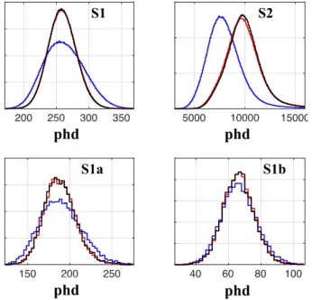
200 250 300 350 phd S1_tot 5000 10000 15000 phd S2_tot 150 200 250 phd S1_32.1 40 60 80 100 phd S1_9.4 effect of correction on Kr83m blue: raw

red: after z-only correction black: after full xyz correction

S1 S2 S1a S1b phd phd phd phd

phd

phd

phd

phd

FIG. 11. The effect of applying the S1 and S2 amplitude

cor-rection maps is illustrated using the83m_{Kr S1 and S2 peaks}

themselves. The starting distribution of uncorrected pulse

area (measured in units of detected photons, phd) is shown in blue, a version corrected only in the z direction is shown in red, and the final version corrected in all three spatial di-mensions is shown in black. The data here is a mixture of

83m_{Kr data sets from a wide range of dates within WS2013}

running, after applying the fiducial volume selection. The

top row shows the quantities used to create the corrections:

83m_{Kr decays for which the two S1 pulses are close enough}

together so as to be treated as a single pulse (tsep <1.2 µs). The lower row shows the individual S1 peaks when separation is achieved in the standard data treatment (tsep>1.2 µs) and serve as a cross check of the S1 correction.

Figure 11 implies that a 3D correction represents only a marginal improvement over a z-only correction. Im-portant variations in xy occur at high radius, outside the fiducial selection used in Figure 11 or in the dark mat-ter search analyses. The improved discrimination when moving from z-only to full 3D correction parameters in Figure 12, then, deserves some comment. This improve-ment is partially a real change resulting from enhanced S1 and S2 resolution, but it is also partly an artifact of the NR calibration’s specific and non-uniform posi-tion distribuposi-tion (the NR calibraposi-tion is performed using a narrow deuterium-deuterium neutron beam [32]). It so happens that the NR calibration distribution on the xy plane is of very slightly enhanced S2 area, leading to an artificially-degraded discrimination measure before the xy corrections are applied.

The83m_{Kr calibrations of position and temporal}

vari-ation lead directly to stronger ER discriminvari-ation and higher sensitivity to dark matter nuclear recoils, and were essential to the analyses published in [20], [21], and [34].

9

0 10 20 30 40 50 60

10-4 10-3 10-2

result of corrections on discrimination, same coloring as correction histograms. todo: investigate improvement from z-only (red) to full xyz (black) and make absolutely sure we believe it.

new, corrected Dec15

S1 [phd]

Le

ak

age

F

rac

ti

on

FIG. 12. A simple metric for background leakage fraction, the fraction of ER events falling below the NR S2/S1 mean,

is shown binned in S1. The ER sample used here is a3H

cal-ibration, the NR sample is a calibration using a deuterium-deuterium (DD) neutron generator. Coloring matches Fig-ure 11: blue denotes uncorrected areas, red denotes a cor-rection only in drift time (z), and black denotes the full 3D correction. Uncertainties illustrated are statistical (√n) alone; S1 values are slightly offset to allow visibility.

VI. USE OF83mKR AMPLITUDE RATIOS TO

MAP ELECTRIC FIELD AMPLITUDE The radial field component described in Section III in-troduces a secondary effect: a drift field amplitude gra-dient in the z direction. Along the central axis, the field amplitude in WS2013 varies from ∼165 V/cm near the plane of the cathode grid to ∼205 V/cm near the plane of the gate grid. A non-uniform electric field amplitude can produce a number of systematic effects, chief among them is a spatially-dependent fraction of electrons which

recombine with ions. A weaker field allows more

re-combination, enhancing the S1 signal and proportionally suppressing the S2 signal. A stronger field has the in-verse effect. Field-dependence is minimal for low-energy electron recoils below 10 keV (where recombination is it-self minimal) and increases above 10 keV [33, 35, 36]. Electric field amplitude variations can also induce other systematic effects, including a spatially-dependent S1 pulse shape (through a varying recombination fraction as in the pulse amplitude case, see [37] and [38]) and a spatially-dependent electron lifetime (through field-dependent capture cross sections, as in [30]). To the extent that these various systematics are important, a direct measure of local electric field amplitude in LXe is advantageous.

The S1 and S2 amplitude correction method described

in Section V assumes83m_{Kr serves as a standard candle,}

and attributes all signal amplitude variation to detec-tor efficiencies and gains. The field dependence of ini-tial photon and electron counts (before detector effects) relaxes the standard candle assumption, introducing a

field-dependent variation that depends not only on event energy but on recoil type (ER or NR). In the WS2013 sci-ence run described here, the scale of the field-dependsci-ence (at all energies and for both ER and NR) is estimated to be few-percent (following [13, 35]), sub-dominant to other uncertainties, and is neglected.

The small field dependence in 83m_{Kr light and charge}

yields can be leveraged to construct a calibration quan-tity that varies with electric field amplitude alone. When

observably separated, the two S1 amplitudes of a83m_Kr

decay (at 32.1 keV and 9.4 keV) exhibit differing field dependence scales. In fact, these two energies form a par-ticularly convenient pair, in that 32.1 keV is well above the O(10 keV) onset of significant field dependence, and 9.4 keV is just below. The ratio of the two S1 amplitudes varies with field alone, since any S1 gain or efficiency ef-fects affect both S1 amplitudes equally.

The result is that the S1b:S1a ratio increases with the field. Figure 13 shows a measurement of this ratio dis-tribution in WS2013. Correspondence of this measured quantity with the field amplitude contours predicted by the field model of Section III is clear. The ratio

mea-surement is statistically limited by the number of83m_Kr

decays for which the S1a and S1b pulses are measurably separated. To maximize useful calibration statistics for

this purpose, the two83m_{Kr S1 amplitudes are measured}

in a special data processing, employing a parameterized fit to estimate the individual amplitudes of slightly over-lapping double-S1 traces. This fit employs two instances of a single pulse template, fitting for four free parameters: two amplitudes and two pulse start times. This method allows S1a and S1b amplitude measurements down to a minimum separation time of 100 ns. This ratio technique for field amplitude measurement is of central importance in subsequent LUX analyses (as in [34]), for which the

field variations in 83m_{Kr recombination are larger and}

require careful treatment.

VII. CONCLUSIONS

This first use of 83m_{Kr in the calibration of a dark}

matter direct-detection experiment takes advantage of

several key attributes of 83m_{Kr: a low-energy}

monoen-ergetic peak conveniently just above the energy region of interest, dispersible uniformly throughout the detec-tor volume, with a convenient hours-scale decay time. The monoenergetic signal enables a precise correction of S1 and S2 amplitudes for position-dependent efficiencies and gains, resulting in an enhanced ER background re-jection ability. The uniform spatial distribution enables a precise reconstruction of vertex position, enabling a well-defined fiducial volume selection. This initial experience with83m_{Kr in a large-scale, operating dark matter} exper-iment pointed the way towards unforeseen uses, such as the mapping of electric field amplitude variation within the TPC. In subsequent LUX operations[34], a buildup of electric charge on PTFE surfaces induced a time-varying

10 0 5 10 15 20 25 Corrected r [cm] 0 50 100 150 200 250 300 Drift Time [ 7 s] S1_9.4 : S1_32.1 10 15 20 25 30 35 40 45 50 55 Bonus plot and prelude for run4: run3 S1b/S1a ratio in the rz plane.

170 V/cm 180 190 200 1 V V/cm V/cm V/cm /cm

D

ri

ft

T

ime

[

µ

s]

Z P

os

iti

on

[c

m]

Radius [cm]

S

1b

: S

1a R

ati

o

Colors correspond to gaussian fits. Areas are from the Kr83m S1 template fit style (for Kr83m S1 pulses separated by small separations), so the areas used here are not the same as in the rest of the paper. That will need be spelled out in the text. Data selection: loose constraint on the ratio, plus separation must be >10samples.

The contours are from a 2D comsol model.

The drift time axis (for the ratio) and the Z position axis (for the contours) are not perfectly one-to-one. The correspond to within 10 samples, close enough for the purposes of this plot.

FIG. 13. The83mKr S1b:S1a ratio, plotted as average values

within bins of drift time and (corrected) radius. S1 ampli-tudes here are measured differently from other ampliampli-tudes in this work, by fitting an S1 pulse template. A gradient in the S1b:S1a ratio is seen, matching the expected variation in field amplitude. The high-field and low-field regions at high radius are also made visible. Field amplitude contours are overlaid using a separate z position axis in cm; correspondence to the drift time axis is accurate within a few percent.

and more significantly inhomogeneous electric field, re-quiring both a more complex procedure for the correc-tion of posicorrec-tions and a more complex approach to S1

and S2 amplitude corrections. These two 83m_Kr-based

calibration efforts, building on the LUX2013 experience described here, will be documented in two forthcoming papers [39, 40]. Work is ongoing to make the most of 83m_{Kr calibrations in current and future projects such as} DarkSide [22], XENON1T [23], and LZ [41].

ACKNOWLEDGMENTS

This work was partially supported by the U.S. Department of Energy (DOE) under award

num-bers DE-AC02-05CH11231, DE-AC05-06OR23100,

DE-AC52-07NA27344, DE-FG01-91ER40618,

DE-FG02-08ER41549, DE-FG02-11ER41738,

DE-FG02-91ER40674, DE-FG02-91ER40688,

DE-FG02-95ER40917, de-na0000979, de-sc0006605, de-sc0010010, and de-sc0015535; the U.S. National Science Foundation under award numbers PHY-0750671, PHY-0801536,

PHY-1003660, PHY-1004661, PHY-1102470,

PHY-1312561, PHY-1347449, PHY-1505868, and

PHY-1636738; the Research Corporation grant RA0350;

the Center for Ultra-low Background Experiments in the Dakotas (CUBED); and the South Dakota School of Mines and Technology (SDSMT). LIP-Coimbra

acknowledges funding from Funda¸c˜ao para a Ciˆencia

e a Tecnologia (FCT) through the project-grant

PTDC/FIS-NUC/1525/2014. Imperial College and

Brown University thank the UK Royal Society for travel funds under the International Exchange Scheme (IE120804). The UK groups acknowledge institutional support from Imperial College London, University College London and Edinburgh University, and from the Science & Technology Facilities Council for PhD stu-dentships ST/K502042/1 (AB), ST/K502406/1 (SS) and ST/M503538/1 (KY). The University of Edinburgh is a charitable body, registered in Scotland, with registration number SC005336.

This research was conducted using computational re-sources and services at the Center for Computation and Visualization, Brown University, and also the Yale

Sci-ence Research Software Core. The 83_{Rb used in this}

research to produce 83m_{Kr was supplied by the United}

States Department of Energy Office of Science by the Isotope Program in the Office of Nuclear Physics.

We thank Kevin Charbonneau at Yale University for

his significant contributions to the dosing of the83m_Kr

generators used in this work.

We gratefully acknowledge the logistical and technical support and the access to laboratory infrastructure pro-vided to us by SURF and its personnel at Lead, South Dakota. SURF was developed by the South Dakota Sci-ence and Technology Authority, with an important phil-anthropic donation from T. Denny Sanford, and is oper-ated by Lawrence Berkeley National Laboratory for the Department of Energy, Office of High Energy Physics.

[1] D. S. Akerib et al. (LUX Collaboration), Nucl. Instrum. Meth. A704, 111 (2013), arXiv:1211.3788 [physics.ins-det].

[2] D. Decamp et al., Nucl. Instrum. Methods A 294, 121 (1990).

[3] A. Chan et al., Nuclear Science, IEEE Transactions on 42, 491 (1995).

[4] V. Eckardt et al., (2001), arXiv:nucl-ex/0101013 [nucl-ex].

[5] J. Stiller and ALICE Collaboration, Nucl. Instrum. Methods A 706, 20 (2013).

11 [6] A. Picard, H. Backe, J. Bonn, B. Degen, R. Haid,

A. Hermanni, P. Leiderer, A. Osipowicz, E. W.

Ot-ten, M. Przyrembel, M. Schrader, M. Steininger, and

C. Weinheimer, Zeitschrift f¨ur Physik A Hadrons and

Nuclei 342, 71 (1992).

[7] A. I. Belesev, E. V. Geraskin, B. L. Zhuikov, S. V. Zadorozhny, O. V. Kazachenko, V. M. Kohanuk, N. A. Lihovid, V. M. Lobashev, A. A. Nozik, V. I. Parfenov, A. K. Skasyrskaya, E. A. Sudachkov, N. A. Titiov, and V. G. Usanov, Physics of Atomic Nuclei 71, 427 (2008). [8] M. Zboril and T. K. collaboration, AIP Conference

Pro-ceedings 1417, 154 (2011).

[9] D. M. Asner et al. (Project 8 Collaboration), Phys. Rev. Lett. 114, 162501 (2015).

[10] L. W. Kastens, S. B. Cahn, A. Manzur, and D. N. McK-insey, Phys. Rev. C 80, 045809 (2009), arXiv:0905.1766. [11] L. W. Kastens, S. Bedikian, S. B. Cahn, A. Manzur, and D. N. McKinsey, Journal of Instrumentation 5, P05006 (2010).

[12] W. H. Lippincott, S. B. Cahn, D. Gastler, L. W. Kastens, E. Kearns, D. N. McKinsey, and J. A. Nikkel, Phys. Rev. C 81, 045803 (2010).

[13] A. Manalaysay, T. M. Undagoitia, A. Askin, L. Baudis, A. Behrens, A. D. Ferella, A. Kish, O. Lebeda, R. San-torelli, D. V´enos, and A. Vollhardt, Review of Scientific Instruments 81, 073303 (2010), arXiv:0908.0616 [astro-ph.IM].

[14] E. Aprile et al., Phys. Rev. D 86, 112004 (2012). [15] T. Alexander et al. (SCENE), Phys. Rev. D 88, 092006

(2013).

[16] H. Cao et al. (SCENE), Phys. Rev. D 91, 092007 (2015). [17] S. Rosendahl et al., Journal of Instrumentation 9, P10010

(2014).

[18] D. S. Akerib et al. (LUX Collaboration), “Position re-construction in LUX,” (2017), in preparation.

[19] J. B. Albert et al. (EXO-200 Collaboration), Phys. Rev. C 95, 025502 (2017).

[20] D. S. Akerib et al. (LUX Collaboration), Phys. Rev. Lett. 112, 091303 (2014), arXiv:1310.8214 [astro-ph.CO]. [21] D. S. Akerib et al. (LUX Collaboration), Phys. Rev. Lett.

116, 161301 (2016), arXiv:1512.03506 [astro-ph.CO]. [22] P. Agnes et al. (DarkSide), Phys. Rev. D 93, 081101(R). [23] E. Aprile et al. (XENON), JCAP 04, 27 (2016). [24] A. Pocar, Ph.D. thesis, Princeton University (2003).

[25] SAES Pure Gas, Inc., “MonoTorr,”

http://www.saespuregas.com/default.aspx?idPage=1113. [26] D. Malling, Measurement and Analysis of WIMP

De-tection Backgrounds, and Characterization and Perfor-mance of the Large Underground Xenon Dark Mat-ter Search Experiment, Ph.D. thesis, Brown University (2014).

[27] COMSOL, Inc., “comsol Multiphysics R

,” http://www.comsol.com.

[28] N. S. Ottosen and H. Petersson, Introduction to the Finite Element Method (Prentice Hall, 1992).

[29] J. B. Albert et al. (EXO-200), (2016), arXiv:1609.04467 [physics.ins-det].

[30] G. Ascarelli, The Journal of Chemical Physics 74, 3085 (1981), http://dx.doi.org/10.1063/1.441402.

[31] L. Baudis, H. Dujmovic, C. Geis, A. James, A. Kish,

A. Manalaysay, T. Marrod´an Undagoitia, and M.

Schu-mann, Phys. Rev. D 87, 115015 (2013).

[32] D. S. Akerib et al. (LUX Collaboration), (2016),

arXiv:1608.05381 [physics.ins-det].

[33] D. S. Akerib et al. (LUX Collaboration), Phys. Rev. D93, 072009 (2016), arXiv:1512.03133 [physics.ins-det]. [34] D. S. Akerib et al. (LUX Collaboration), Phys. Rev. Lett.

118, 021303 (2017).

[35] M. Szydagis, N. Barry, K. Kazkaz, J. Mock, D. Stolp,

M. Sweany, M. Tripathi, S. Uvarov, N. Walsh, and

M. Woods, Journal of Instrumentation 6, P10002 (2011). [36] D. S. Akerib et al. (LUX Collaboration), Phys. Rev. D

95, 012008 (2017).

[37] K. Ueshima, , et al., Nucl. Instrum. Methods A 659, 161 (2011).

[38] D. S. Akerib et al. (LUX Collaboration), “Scintillation pulse shapes and pulse shape discrimination in a large liquid xenon time-projection chamber,” (2017), in prepa-ration.

[39] D. S. Akerib et al. (LUX Collaboration), “3D modeling of electric fields in the LUX detector,” (2017), in prepa-ration.

[40] D. S. Akerib et al. (LUX Collaboration), “Corrections to the LUX WIMP search data in the presence of a non-uniform electric field,” (2017), in preparation.