1
Basic Income and Minimum Income: a Portuguese Case
Analysis of Past Basic income Experiences and Consequences of a Potential
Introduction in Portugal
Diogo Vicente
Thesis written under the supervision of Prof. Maria Isabel Horta Correia
Dissertation submitted in partial fulfillment of the requirements for the degree of MSc in Economics at the Universidade Católica Portuguesa, 03rd of April, 2017
2
Abstract
English VersionThe idea of Basic Income has gained ground around schoolers and public authorities. Several experiments have been conducted over the last decades with interesting results being observed. At the same time Minimum Income Schemes across, the most similar type of policy in place, seem incapable of achieving their proposed goals. This work selects four Basic Income experiments and compares their results with the results of the Portuguese Minimum Income Scheme. It shows that the Portuguese current Scheme does not fully accomplish its proposed goals of reducing poverty while promoting inclusion. Moreover, it is demonstrated that Basic Income Experiments delivered motivating results both in terms of shrinking poverty and stimulating labor. This work argues that the current Portuguese Minimum Income Scheme needs a remodeling and that the idea of Basic Income should be considered as an alternative policy.
Portuguese Version
A discussão à volta da implementação de um Rendimento Básico Universal tem ganho adeptos junto de investigadores e entidades públicas. Várias experiências foram levadas a cabo nas últimas décadas, produzindo resultados interessantes. Simultaneamente, as políticas de Rendimento Mínimo em vigor – o tipo de política que mais se assemelha a um Rendimento Básico Universal – têm sido incapazes de cumprir os pressupostos em que foram fundados. Este trabalho seleccionou quatro experiências com Rendimento Básico Universal e comparou os seus resultados com os resultados produzidos pelo esquema de Rendimento Mínimo Português. É demonstrado que o esquema Português não é capaz de cumprir os objectivos a que se propõs quer a nivel da redução de pobreza, quer na ajuda à inserção social e profissional. É ainda evidenciado que as experiências de Rendimento Básico Universal foram capazes de mitigar os indíces de pobreza enquanto promoviam o emprego e a inclusão. Este trabalho considera que o esquema de Rendimento Mínimo Português necessita de ser reconfigurado e que a ideia de um Rendimento Básico Universal devia ser considerada como uma possível política alternativa.
3
Acknowledgements
First of all I would like to thank Professor Maria Isabel Horta Correia for always finding the time to answer my questions and doubts and for all the valuable advice and inputs throughout these months.
I want to thank my entire family for all the support throughout the process. To you Sandra, Leonor and Jorge for helping more than ever in this stage, to you Luis, Cristina and Americo for your help on what led to here. To all the Quaresmas who always brough the bright side. To you Anela Alic for nothing and for everything.
To you Gloria Morgado for being the most amazing human being I have ever had the pleasure to meet.
4
Table of Contents
Abstract 2 Acknowledgements 3 List of Figures 5 List of Graphs 5 List of Tables 6 1. Introduction 7 2. Literature Review 92.1 - A Brief History of Basic Income 9
2.2 - Basic Income vs Minimum Income 10
2.2.1 - Basic Income vs Minimum Income: Poverty – A Fair and Equal Society 11 2.2.2 - Basic Income vs Minimum Income: The Labor Market 13
3. Basic Income Experiments 18
3.1 – Introduction 18
3.2 –Poverty 20
3.3 – Labor Market 25
4. Minimum Income Scheme vs Basic Income – A Portuguese Case 33
4.1 Introduction – 33
4.2 Poverty – 36
4.3 Labor Market – 40
5. Conclusions 44
5 List of Figures
Figure 1 - Conditional vs Unconditional Welfare System………...11
Figure 2- Introduction of Minimum Income………...14
Figure 3 – Introduction of Minimum income – t=1………...15
Figure 4 – Effects of Increasing G………...15
Figure 5 - Effects of reducing t………...16
List of Graphs Graph 1 - BIG Namibia Poverty Indicators………...21
Graph 2- BIG Namibia – Income………..21
Graph 3 - Mhadya Pradesh Changes in Income………....22
Graph 4 - Alaska Poverty Rates………....23
Graph 6- Mhadya Pradesh - Shift in work activity………...26
Graph 6 - Mhadya Pradesh- Employment………...27
Graph 7 - BIG Namibia- Unemployment………..28
Graph 8 - RSI Evolution – Individuals vs Amount………...34
Graph 9 - RSI as % of Social Security Expenditure………..34
6 List of Tables
Table 1 – Income and Substitution Effects………...17
Table 2- US NIT Experiments………..19
Table 3 - BIG Income Sources………..21
Table 4 - Mhadya Pradesh - Treatment Group……….22
Table 5 - Mhadya Pradesh - Control Group……….22
Table 6 - NIT – Predicted Poverty Effects for all Experiments………24
Table 7 - Mhadya Pradesh - Changes in Labor……….25
Table 8- NIT- Husbands Labor Response ………29
Table 9- NIT- Wives Labor Response………...29
Table 10- NIT- Single Female Heads Labor Response……….29
Table 11 - NIT Employment Response………..30
Table 12 - RSI Sample vs Portugal - Employment Data………...35
Table 13 - RSI Effects on Poverty………...36
Table 14 - RSI Efficiency Indicators……….38
Table 15 - RSI Contracts Terminated by Motive………...39
Table 16 - % of RSI Beneficiaries working - When claimed vs Now………...40
Table 17 - RSI Beneficiaries by Situation – Working when RSI was claimed and Now………..41
Table 18 - RSI - Did you have any job offer in the last year?...41
Table 19 - RSI - Last time you looked for a job?...41
7
1. Introduction
Data shows that the world has never been wealthier (World Bank, 2017) and the last decades presented an outstanding decrease in extreme poverty. This reduction was particularly remarkable in nations that enjoyed explosive growth such as those in the regions of East and South Asia. However, as of 2011 around 14% of the world population was still severely poor. In addition, the recent financial crisis and the economic deceleration that followed caused some setbacks on this matter. For example, in the period between 2007 and 2014, out of the 35 members of OECD, 21 saw an increase in the share of population below their poverty threshold (OECD, 2017). In line with this recent trend, we observe a rise in market inequality income in both developing and developed nations (ibid). The consequences of inequality and poverty on matters like social mobility, growth, crime, or education have been more or less unanimous among literature (Berg et al, 2014; Corak, 2013; Fajnzylber et al, 2002). It is undisputed that a society which struggles to grow, has low social mobility, increasing levels of crime, and in which education is not efficient is one where freedom and individual justice are endangered. Justice is a fundamental matter in every society. It is as John Rawls stated “the first virtue of social institutions” (Rawls 1971, 3). Although potentially skeptical about a Basic Income (Noguera et al, 2013), Rawls’ Liberal-Egalitarianism is a trend followed by most supporters of Basic Income (BI) and the moral substance of the idea. This idea gained momentum with all of the above leading to a growing discussion about the concept and its potential. We have seen experiences being conducted at smaller scales throughout the world with interesting results. The closest idea that current welfare policy uses at large scale is Minimum Income (MI). This policy was first developed over 50 years ago and it is now used in most developed regions and some under-developed nation with the goal of alleviating poverty and promoting employment. However, we will see that its success in doing so can be questioned. For this reason and given the similarities between a Minimum Income and a Basic Income in terms of essence and goals I believe that developing a work that allows us to revisit some of the most thorough BI experiments ever conducted in connection with an analysis about the current Portuguese MI scheme can be valuable. It will allow us not only to understand better the effectiveness of the Minimum Income policy in Portugal, but also to comprehend the potentialities of a BI in the country in a time where several cities and authorities around the world are developing and implementing pilots of the scheme. Given that the goals that were on the base of implementing Minimum Income Schemes are related
8
with the subjects of Poverty and Labor Inclusion, I will perform my analysis by covering these two topics and the potential effects of the two measures on both.
A couple of limitations need to be considered. I will use the BI definition in Van Parijs (1995) – a universal and unconditional, no-means tested benefit which is big enough to cover a individual’s basic needs - but since only a limited number of BI experiments were ever conducted, the width of choice is reduced and some of the BI assumptions that my definition uses will need to be withdrawn. Also, the BI experiments selected for the purpose of this work were not exactly intended to answer the questions I aim to respond here. Thus at some moments conclusions will need to be taken carefully and data will have to be examined in an indirect way.
I do not expect to provide full and straight answers, but what I intend and hope to do over this work is to contribute to the debate on Basic Income and help to raise questions regarding the status quo of current welfare policy.
9
2. Literature Review
2.1 - A Brief History of Basic Income
In this first chapter I will briefly go through the history of Basic Income. My aim is to point out the most important contributions to the matter over the last 500 years, but also to show that the issues that are at the center of discussion today have been under argument since the first theory on BI was developed.
To track back the first ideas on a BI we have to travel to the Renaissance. In the 16th Century Thomas More and Johannes Ludovicius Vives, on discussing justice and equality, would draw the very first ideas about the subject. It was in order to address crime and poverty that the concept was first developed.1 The authors saw BI as a potential response for such issues, and Vives, the “father” of BI drew the first proposal. His plan would be financed by the local government and be mainly targeted to the poor with the condition that the entitled person would be willing to work2. A new approach is observed in the 18th century when Thomas Paine, brings the concept of universality to the table. Paine’s vision was that land is common property of all men, and that for this reason, those who own land were in debt to the rest of the community. Hence, a BI should be universal and funded through a so called “ground rent”3 that these owners owed to the community (King & Marangos, 2006).
Bertrand Russell, in accordance to Paine’s vision, designed in the 20th century his own plan on a BI. Such plan would be divided in two: a small income, secured to all whether or not they work, and a bigger transfer that should be awarded to those who engage in activities who are to be considered, useful by the community4.
This universality continues in the 20th century with Nobel Laureate James Meade. In his work on the subject, which lasted his entire career, being lastly presented in Agathotopia5, Meade
1 More was openly against death penalty, claiming that “Instead of inflicting these horrible punishments, it
would be far more to the point to provide everyone with some means of livelihood” Source: Adams, R & Logan, G (eds) 2002, Utopia, Cambridge University Press, Cambridge.
2 Source: Tobriner, A (ed) 1999, On the Assistance to the Poor, Reinassance Society of America, Canada. 3 In a pamphlet written in 1797 called Agrarian Justice, Thomas Paine describes ground rent as a tax that should
be paid by land owners once by generation. Paine proposes a 10% tax on direct inheritances, and a higher rate for indirect inheritances.
4 Source: Russell, B 1996, “Work and Pay”, in Proposed Rods to Freedom, Project Gutenberg Etext, viewed 23
September 2016
5 The word comes from the merge of the words Agathos, which means good, and Utopia. It would describe a
place that would be good enough to live in, opposing to Thomas More’s Utopia, where the author describes a perfect but unreachable model of society
10
proposes a “social dividend”, which should be unconditional and equal to every citizen. According to the Nobel Prize winner, the dividend would be the right tool to alleviate poverty and to crear a more just and efficient economy.
In the second half of the century Milton Friedman propposed the idea of a Negative Income Tax (NIT) as a new policy on social welfare6. Since I will describe some NIT experiments later on seems sensible to explain briefly how does a NIT work. The State defines a certain threshold and households whose income falls below that threshold are awarded a subsidy. The size of the subsidy would depend on the established tax. If for example the threshold was defined at 5000$ and the household or family had a total income of 4000$, then for a tax of 20%, the subsidy would be 200$. This is the result of applying the 20% tax to the gap between the earned income and the border defined by the government (Moffitt, 2003). Friedman’s idea brought attention to the subject of BI in the US and in 1968, James Tobin, Joseph Pechman and Paul Samuelson were amongst a group of 1200 economists who signed a document calling for the Congress to introduce a system of income guarantees. The proposal would ultimately be rejected by the Senate but opened room for the first experiments around the world, and launched the discussion in Europe.
As I stated in the introduction of this chapter, what the history of BI tells us is that today’s questions regarding the proposal are the ones that were raised by most authors in the past. From More’s concern on Labor supply effects, to Paine’s method of funding it. Russell’s vision on freedom or Friedman’s approach on welfare systems are all items under discussion today. Such subjects are the Nemesis of a BI, and henceforth the topics that I intend to discuss in this work.
2.2 - Basic Income vs Minimum Income
In this section I will review what the literature says about the theoretical effects of Basic Income and Minimum Income over the subjects under analysis in this work: Poverty and the Labor Market. In order to better understand the two policies and their potential consequences let me briefly describe their proposals and its differences. A Basic Income, as I stated before, is in the definition I am using here a no means-tested universal cash benefit. It is awarded to
6 The Negative Income Tax (NIT) idea was first ever proposed in his book Capitalism and Freedom, but was
constantly developed throughout Friedman’s career. The Nobel Laureate saw NIT as a solution to eliminate the welfare trap and develop an incentive to work for those under state assistance. Moreover the policy would also allow for a reduction in Bureaucracy and Administrative Costs raised by all the multiple programmes that were and still are today in place to assist the poor.
11
every citizen regardless of income or work situation and its amount is similar to all citizens (Van Parijs,1995). On the other hand a Minimum Income is a benefit awarded to those households who fall in the poorest deciles of society as a measure of providing a safety net below no one should fall. The subsidy covers a gap between the individual’s income and a certain amount that the State considers as a fair amount under which no citizen should live on. The measure is usually linked to an inclusion goal and beneficiaries are often obligated to either perform work or pursue some type of training.
2.2.1 - Basic Income vs Minimum Income: Poverty – A Fair and Equal Society
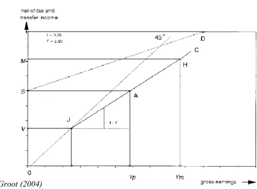
Current poverty rates are one of the main arguments of BI supporters. They believe that through Basic Income we are able to reduce more effectively the incidence and severity of poverty. By being unconditional, BI breaks the link between work and income and could ultimately interveen amongst those who fall in the poverty trap that current welfare creates. To comprehend this argument better let us compare the two schemes regarding earned and unearned income. Fig. 1 shows us the differences between conditional and unconditional benefits in the presence of a minimum wage. Given that Portugal, the nation under analysis, falls in this category – a conditional transfer in the presence of a minimum wage – the example seems relevant.
Figure 1 - Conditional vs Unconditional Welfare System
12
On the horizontal axis we have gross labor earnings and on the vertical axis we see net of tax and transfer income. The line S̅D̅ represents the unconditional benefit – Basic Income - summed to the minimum wage with a single tax rate equal to 𝑡 = 60%. It is important to note that there is a difference between the withdrawal rate and the rate applied to earnings. The first represents the percentage of every extra dollar earned captured by the scheme. The second is just the usual tax rate on earnings. The line S̅A̅H̅C̅ represents the conditional benefit. The point S represents the social minimum amount, meaning the value that the State defines as the one that no beneficiary should fall below. In the BI case we have a flat tax rate 𝑡 = 60% while on the other, the rate is 𝑡 = 25%, taking into account the potential costs of each policy7. With a conditional system those who are unemployed get earnings equal to the line O̅S̅. For a withdrawal rate of 100%, like in the Portuguese case, meaning every extra euro earned above the level S is captured, those who are employed under the conditional system, stay in the line S̅A̅, the poverty trap line, until their revenue is bigger than 𝑌𝑝8. The poverty trap means that if a person is under the conditional assistance it does not compensate to perform any work that does not raise the earnings above that level. In the graph we see that the benefit is only a little below the amount defined as Minimum wage, 𝑀. This is usually the case in countries that support the two policies (Frazer&Marlier, 2016). Given that most people who face this poverty trap are under qualified, meaning low skilled, and are unable to find a job that pays a salary much higher than the ruled minimum wage, there is usually no escape from the trap9. With a BI programme, the poverty trap disappears given that as line S̅D̅ shows, every extra euro earned is not absorbed, although to be sustainable the flat tax rate considered should be raised (in this case t’=60%). Since every citizen would receive the benefit, the system would generate net earners and payers, depending on the amount of earned income. In the end of the day, given that the flat tax rate would suffer a substantial increase it is straightforward that most households woulde be net-payers and thus would be worse off. However, when we compare the two we see that if the social minimum amount is kept as the same level, no one would fall below this level with BI. Moreover, since the line S̅A̅
7 It is worth mentioning however that although costs could increase with a basic income delivered to everyone
the bureaucratic costs would be highly reduced given that the programme would be no means-tested. Moreover there would be no possibility of giving the benefit to someone who should not be entitled to it
8 It is relevant to notice that in the Portuguese case the line S̅A̅, depends on the type of household or famlily.
Given that when calculating the minimum amount a household or family should receive, the State takes into account the family’s composition, each family will have a different threshold. Hence the line S̅A̅ will vary across the population
9 In Portugal for example, the percentage of Minimum Income beneficiaries’ who have secondary or higher
13
disappears, everyone that was on the poverty trap before and decides to engage in paid work is awarded with a net income above the level permitted with Minimum Income.
The transition to a BI in the terms here propposed is not Pareto efficient and would raise discussion over the issues of justice and reciprocity. However, it is clear that BI presents a better model to tackle poverty amongst the lowest deciles of society. By eliminating the poverty trap that current Welfare promotes, BI is able to allow all of the households who were under this trap to increase their net earnings through paid work and at the same time avoid for any of them to fall below the social minimum that was already fixed.
2.2.2 - Basic Income vs Minimum Income: The Labor Market
We have seen in the previous chapter how by eliminating the poverty trap, BI could create an incentive for the unemployed under assistance to perform paid work. However, given that the scheme would no longer be conditional or means-tested – like in the case of a Minimum Income - and that the amount delivered would be enough to cover the beneficiary’s basic needs, an impact on the labor market should be expected. Critics of the scheme often claim that the incentive to work would be strongly reduced, thus a decrease in the number of hours worked would be observed, and that this would result in a complete remodeling of the labor market (Anderson & Block, 1993). In this chapter I will analyze these concerns. To make the analysis more harmonious I will adapt the model used in Moffitt (2002).
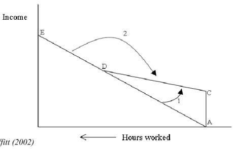
The model goes as following: the individual chooses Leisure(𝐿) and Consumption (𝐶) with a budget constraint equal to 𝑃𝐶 = 𝑁 + 𝑊(𝑇 − 𝐿). 𝑃 being the price, 𝑁 the unearned income, 𝑊 is the wage rate and 𝑇 is the total time available. If we consider Hours of work, 𝐻, as 𝐻 = 𝑇 − 𝐿, then the individual will choose his utility over the function 𝑈(𝐻, 𝑌), maximized to 𝑁 + 𝑊𝐻 = 𝑌. Adding now a benefit 𝐵 = 𝐺 − 𝑡(𝑊𝐻 + 𝑁) we have a new budget constraint equal to 𝑊 (1 − 𝑡)𝐻 + 𝐺 − 𝑡𝑁 = 𝑌. G is equal to the amount given to those with zero income – in fig.1 this would be the equivalente to 𝑆 - and 𝑡 is the marginal tax rate. Minimum Income and Basic Income will differ on the size of 𝐺 and the marginal tax rate 𝑡 used. Over the next sections I will analyze what are the different results of changing these variables.
I would like to start my analysis with the implementation of a Minimum Income from scratch. Fig.2 shows the results of this implementation
14
Figure 2- Introduction of Minimum Income
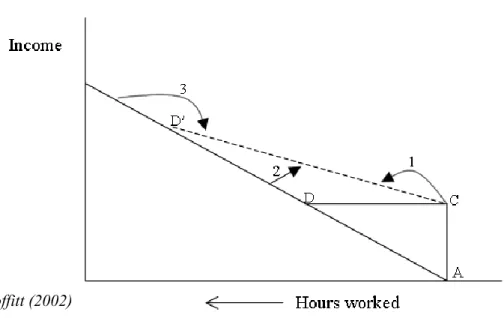
𝐶𝐷 represents the budget constraint 𝑊 (1 − 𝑡)𝐻 + 𝐺 − 𝑡𝑁 = 𝑌. The line 𝐶𝐷 intersects 𝐴𝐶 at the point defined in the model as 𝐺. 𝐴𝐸 is the constraint for an economy with no welfare policy in place. The arrows 1 and 2 show what the consequences of introducing the measure to both people earning an amount below and above the level are. If they earn an amount that is located below D, in the line AD, that means that they are better off by being under welfare assistance even if they reduce the numbers of hours worked. For people above the level 𝐷 they would still reduce the number of hours worked eventhough they would face a reduction in their income. In this example the marginal tax rate is equal to the slope of 𝐶𝐷, meaning −𝑊(1 − 𝑡). However, it is usually the case where 𝑡 = 1. Fig. 3 shows that the results are similar for that case. In this figure we have an example of the transition from a regime with no Minimum Income Scheme in place to a regime where a Minimum Income is delivered with a marginal tax rate, 𝑡=1.
15
Figure 3 – Introduction of Minimum income – t=1
Until the worker is able to go above the break-even point he has no incentive to enroll in labor activities. As I stated above, introducing a BI presents a different structure, not only because the benefit becomes universal but also because the amount distributed to each individual is substantially higher and the marginal tax rate on the transfer is zero (although as we saw the flat tax rate actually increases to make up for the cost). Let us understand now how a change in G, the value of the benefit, affects the dynamics.
Figure 4 – Effects of Increasing G
In the scenario described by Fig.4 we are still dealing with a marginal tax rate 𝑡 < 1. The consequences of increasing the amount distributed by the programme are similar to those we saw with the introduction of Minimum Income. Regardless of the amount earned by the
Source: Cowen & Tabarrok, 2015,
16
individual we will witness a reduction in the numbers of hours worked. In the case of arrow 3 this is the sole result of an income effect. In the other two cases the income and the substitution effect run in the same direction resulting in a decrease of labor supply that still brings a higer income than before. Finally let us see the dynamics that a change in 𝑡 produce with the help of Fig.5.
Figure 5 - Effects of reducing t
In this example we see a marginal tax rate equal to 1. If we reduce this rate we observe what we should expect based on the previous section analysis. Those who were in the region 𝐶𝐷 will now increase their labor supply given that the the reduction on the extra earnings they obtain through paid work are not fully retained anymore. This is the reasoning behind other alternatives proposed to replace Minimum Income schemes or other welfare policies such as the Negative Income Tax or the Earned Income Tax Credit10. However, those who were just slightly above this region will tend reduce their work effort. For those who were comfortably above the mentioned level a reduction in the number of hours worked will be translated into a descrease in earnings. For the former we are in the presence of an income effect working solely. For the latter we are once again having a substitution and an income effect running together in the same direction.
Let us now center our attention at the effects observed for those with an income that falls in or close to the line 𝐴𝐷. As we saw one should expect a negative substitution effect as a result of
10 The Negative Income Tax was already explained in detail.The Earned Income Tax Credit as the name suggests
is a tax credit. This credit is a share of the worker’s earned income. The share grows as the individual’s income rises until a certain point where it stagnates and then starts to phase out. The credit rate and the maximum value is calculated based on the individual’s family composition (Scholz, 1996).
17
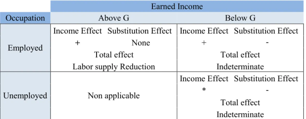
increasing 𝐺 or decreasing 𝑡. This is true for both working and non-working beneficiaries. The income effect runs in the case of increasing 𝐺, in the same direction of the substitution effect. On the other hand for a decrease in 𝑡 we observe that those who were at point 𝐶 end up increasing the number of hours worked or at least not reduce them since there is no incentive in doing it. When introducing a BI in a welfare system that currently offers a Minimum Income with the usual marginal rate of 100% this is exactly what one should expect even though the marginal rate in this case will be 𝑡 = 0 and not 0 < 𝑡 < 1. Table 1 summarizes the potential income and substitution effects that could arise depending on the beneficiaries’ situation and income.
Table 1 - Income and Substitution Effects
Earned Income
Occupation Above G Below G
Employed
Income Effect Substitution Effect Income Effect Substitution Effect
+ None + -
Total effect Total effect
Labor supply Reduction Indeterminate
Unemployed Non applicable
Income Effect Substitution Effect
* -
Total effect Indeterminate
Labor Market effects are hard to measure. Several variables need to be taken into account and models often contain unreasonable assumptions. Nevertheless this chapter had the goal to explain the main topics that are at the center of attention when debating the impact of BI on Labor Market. The size of the benefit as well as the individual’s preferences need to be taken into account when analyzing the potential labor supply results of introducing a BI.
Notes: + Positive effect ; - Negative effect ; * Depends if leisure is perceived as normal or inferior good
18
3. Basic Income Experiments
This chapter will be dedicated to visit four Basic Income Experiments that were conducted over the last half century: the US NIT experiments in the 60’s/70’s; the Alaska Permanent Fund; the Mhadya Pradesh experiment in India; the Namibia BIG experiment.
As stated in the introduction, the lack of BI examples leads us to widen the choice in terms of the programme characteristics. Apart from Alaska, the US experiments were based on a Negative Income Tax and the trials in Africa and India deal with a completely different background from the one we have in Portugal. However I believe that each example provides valuable data to our work and that each programme will offer comparable figures that will allow for several suggestions to the Portuguese case. Furthermore I decided to present 2 experiments from both developed and under developed countries so that not only potential comparisons can be made to the Portuguese case but also to understand how different are the results for the two types of realities.
To be coherent with my work I shall analyze these experiments not case by case but by looking at their results jointly at the areas under analysis in this work: Poverty and Labor market.
3.1 – Introduction
Before starting examining the results of the selected experiments let me briefly characterize them in time, space and design.
US experiments:
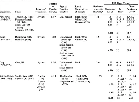
The US experiments were conducted in 4 different regions of the United States over the 60’s and 70’s. They were based on the idea of a Negative Income Tax (NIT) first proposed and developed by Milton Friedman11. A NIT is relatively different from a BI in the sense that it is not unconditional or universal. However analyzing these particular trials can be important for this work for the results they can deliver on fundamental matters such as labor supply response. The amount of the benefit varied from 50% to 150% of the poverty line threshold amount. A full summary of the experiment conditions can be seen with Table 2. All of the trials contained both an experimental group and a control group.
19
Table 2- US NIT Experiments
Madhya Pradesh, India
In the region of Madhya Pradesh 6000 people from 9 different villages were granted with an average payment of $USD 24 per month. The amount was the equivalent to a quarter of the income of the median-income family, which was roughly equivalent to the poverty line. The transfer occurred for a period from 12 to 17 months between June 2011 and November 2012. It was developed in a partnership between UNICEF and a local women’s association named the Self Employed Women’s Association (SEWA). 12 other villages were treated as a control group.
Alaska Permanent Fund:
The Alaska Permanent Fund was established in 1976 based on oil revenues. The fund pays a yearly dividend to every citizen based on a 5 year average performance. This dividend comes really close to our definition of UBI in the sense that it is no means-tested, universal and individual. It is the only BI experiment that was not time lined. The dividend amounts on average to US$2000, a sum that represents roughly 6% of the average personal income.
Source: Robins (1985)
20
BIG Namibia:
The BI trial in Namibia was conducted from January 2008 to December 2009, with all Otjivero-Omitara (area in Namibia) residents, who were under 60, being given N$100 per month, an amount only N$18 below the average per capita income of N$118. This experiment was developed by the Namibian BIG (Basic Income Grant) Coalition, a group formed by several Namibian NGO’s.
3.2 –Poverty
As we saw earlier in this work, current poverty rates on both developed and under-developed countries are one of the main arguments of BI claimers. From the four experiments we are here analyzing, only the ones that were conducted in Namibia and India had amongst their primary goals to fight poverty. Nevertheless in all of the trials here presented, we can draw conclusions on the subject either by a direct analysis on poverty indicators or by examining the behavior of other variables that can relate to the topic.
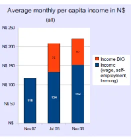
In Namibia almost the entire population was poor12. Before the project started 97% of people were severely poor and 72% were below the food poverty line (Graph 1) .The first immediate consequence was a drop in those numbers. Just after a year, those with food deprivation were now 16% and those facing severe poverty were 43%13. This was accompanied by reductions on child malnutrition – 42% to 10% - (Making the Difference – The BIG in Namibia, 2009, p.53). Moreover income rose. Not only income provided by BIG, but that from wages and self-employment (Graph 2). The latter expanded from N$118 to N$154, a 30% increase. As for Self-employment there was an increase in income from this source of 301% (Table 3). All of these results can be seen below.
12 The poverty line in Namibia was at the time set at N$316 per month. The Namibian GDP per capita at PPP
was $7850 in 2008, roughly 1/7 of the US GDP per capita at PPP.
13 These numbers were controlled for migration, given that several people moved to the area, even though they
21
Graph 1 - BIG Namibia Poverty Indicators Graph 2- BIG Namibia - Income
Table 3 - BIG Income Sources
The reports from Madhya Pradesh do not examine the usual poverty indicators. Hence we will analyze other important poverty measures and compare them between experiment and control groups bearing in mind that the benefit was roughly a quarter of the income generated by a median-income family. A first indicator is children’s weight. As we can see through Table 4 and Table 5 at the beginning of the trial, BI villages had 60.8% of children underweight against 52.1% in control villages. At the end the number with the BI population dropped to 41.1% and decreased to 41.8% amongst the control children.
Source: Making the Difference – The BIG in Namibia (2009)
22
Table 4 - Mhadya Pradesh - Treatment Group Table 5 - Mhadya Pradesh - Control Group
Let us now look at how earned income changed for both groups. 21% of those receiving BI claimed they increased their earned income against 10% who say their income decreased (Graph 3). On the other hand for the control group, 19% saw their earned income decreasing and only 9% enjoyed a rise in their revenue.
Graph 3 - Mhadya Pradesh Changes in Income
In the North-American experiments the background and focus was different. Given this let us look at some of the indicators on this topic. In Alaska the dividend did reduce poverty, but
Source: Piloting Basic Income Transfers in Mhadya Pradesh, India(2014)
Source: Piloting Basic Income Transfers in Mhadya Pradesh, India(2014)
Note: There is here a distinction from SEWA and Non-SEWA depending if the association was active in that village
23
after an initial drop in the first years – In 1979 the poverty rate in Alaska was 10.8%14 (Danzinger&Ross, 1987) - rates have been increasing over the last 25 years. Graph 4 shows that poverty rates decrease by an average of 2% due to the dividend but those rates have rose in all Alaskan areas. The problem is more complex in the rural areas, where most native Alaskans live and where jobs are scarce and the economy is highly based on agriculture. It needs to be taken into account that Alaska is not the only state where poverty has risen. Right before the dividend started being distributed the US average poverty rate was 11.6%, a number very close to the Alaskan one. Today the US rate is 14.8% against a share of 11.4% of Alaskans being poor. Furthermore in 1979 Alaska was the 26th state with the lowest poverty rate and today it is the 8th state dealing with the smallest incidence of poverty (US Census Bureau, 2017).
Graph 4 - Alaska Poverty Rates
Regarding the NIT experiments, results on poverty are harder to infer from and need special caution on examining them. There is no direct data evaluating the evolution of poverty rates in the areas covered by the benefit. Nevertheless the final reports on these experiments when existent, do evaluate the changes that such a programme could produce taking into account the potential dissolution of other State assistance schemes. Poverty rates vary according to the type of help provided and the family under assistance as Table 6 shows. For example, single female headed families would always be worse off. This has to be seen in context. These tests were conducted about 40 years ago and the labor market composition was significantly
14 In the United States the poverty line is defined by the US Census Bureau at a threshold that corresponds to
three times the cost of a minimum food diet.
24
different from now with female participation rates exploding ever since. In 1970 female participation rate was 43.3% and in 2014 it was 57%15. With female participation in the labor market still low, dependence on State help was high for this type of family. On the other hand results for more traditional families at the time - husband-wife families – were expected to be virtuous. Poverty rates would decrease in one of the benefit types and the poverty gap would substantially diminish in both of the scheme forms.
Table 6 - NIT – Predicted Poverty Effects for all Experiments
Results on poverty are shown to be fairly positive. For under-developed regions we see that people whose situation involved being deprived from the most essential resources, used the benefit to access those resources rather than exhausting the money in a less “ethical” way. Moreover and perhaps more important we see that beneficiaires used the contribution in such a productive way, that they were able to increase their own earned income. This shows that a BI has the potential not only to temporarily reduce poverty through the income boost provided but eliminate it due to the incentive of consuming the benefit in a productive way. In the United States results were slightly different. The dividend does indeed reduce poverty rates in Alaska in a still considerable way. As for the NIT experiments results were less exciting. Nevertheless we need to take into account the timing of the experience as well as its characteristics in terms of people covered and conditions offered.
15 Source:Status of Women in the States, viewed 9 February 2017,
<https://statusofwomendata.org/earnings-and-the-gender-wage-gap/womens-labor-force-participation/>
Source: Source: Final Report of the Seattle-Denver Income Maintenance Experiment – Volume – 1 (1983)
25
3.3 – Labor Market
To discuss the sustainability of a BI one needs to discuss its impact on the Labor Market. Defenders claim it is a way to provide fair and decent access to the most neglected ones, opponents fear that such a measure could create harmful new dynamics by eliminating the incentive to work and reducing labor supply. The experiments under analysis here provide important data on several aspects of the Labor Market. The NIT experiments were mainly developed to test the response of low-income families in respect to labor participation. Hence extended data is available to evaluate how these bottom decile households behave in the presence of such an incentive. The schemes developed in the underdeveloped regions had the aim of alleviating severe cases of starvation but also provide valuable information on how those who are more in need react in terms of consumption, labor supply responses and education. Thus several conclusions can be taken regarding the subject of labor market in those experiments.
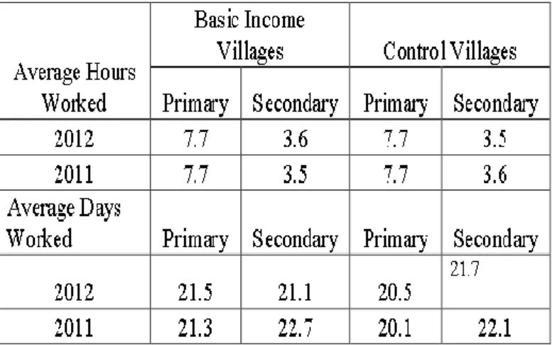
In India, as we can see with Table 7 the number of hours worked in both the primary and the secondary activity16 met no alteration. Results are similar for control and treatment populations. The number of days spent at work per month saw a small change with a bigger focus on the main activity and a little decrease in the secondary activity.
Table 7 - Mhadya Pradesh - Changes in Labor
16 The report on Madhya Pradesh defines two types of activities based on the time spent: the main one which is
the one that the household devotes more time to, usually paid work for others; a secondary activity that takes less time and that can include paid and unpaid work such as housing activities or farming.
Source: Piloting Basic Income Transfers in Mhadya Pradesh, India(2014)
26
Looking now more deeply at what those main activities are. Graph 5 shows that the biggest shift that occurred in both groups was in the share of those working on own account. This happened mainly due to a reduction in terms of casual work for wages in the case of the experimental group and the decrease in the share of people in the control group who worked for wages as regular employment. Finally we shall see how did the labor market evolved in more generic terms regarding the household status before and after the benefit with the help of Graph 6. Although somewhat small, differences between groups confirm what one should expect. For those receiving the benefit, there was an increase in the group of people working for pay, which leads me to believe that they took advantage of the situation and created an opportunity to increase their gains. This led to more people in this group that were not employed due to housework or family care, possibly making use of the extra profit. Finally two important numbers arise from this figure. First, the share of people who were not working because they were attending some training or education decreased. Second, those unemployed and seeking for work were now less, which can mean that this benefit lead to a disincentive to pursue a work activity.
Graph 5 - Mhadya Pradesh - Shift in work activity
Source: Piloting Basic Income Transfers in Mhadya Pradesh, India(2014)
27
Graph 6 - Mhadya Pradesh- Employment
Data in Namibia regarding this topic is less extensive. However there are still two interest indicators to analyze. Graph 7 shows the evolution of unemployment rates in the region during the programme. We see that unemployment rate dropped from 60% to 45%, with employment rising from 44% to 55%. Although no concrete data exists on whether the benefit brought a reduction in the number of hours worked, ultimately we know that the incentive got more people into the labor market. Given that as we saw earlier the personal income excluding the benefit increased it is fair to assume that even if the number of hours worked did indeed decrease, productivity gains were observed. Thus no real disincentive was created with the scheme. What the report on this experiment can also tell us is how the source of household income changed with the programme. As we saw before with Table 3 there was a blast in terms of revenue from self-employment. Moreover we see that although in a shyer way, all items enjoyed an increase with the exception of remittances, clearly a sign that less support was needed from family members of other regions17. This increase in self-employment, as reports state, was due to the small enterprises that emerged in areas like clothing manufacturing or retailing. Their appearance was only possible as a result of the demand boost and start-up capital that was provided by a Basic Income.
17 It is worth mentioning that inflation was around 9%, meaning that even taking inflation into account there was
a clear boost in the economy due to the benefit
Source: Piloting Basic Income Transfers in Mhadya Pradesh, India(2014)
28
Graph 7 - BIG Namibia- Unemployment
In Alaska the labor supply response to the dividend was almost insignificant. When asked if there was a reduction in the amount of time spent working for pay, only 1% of the people answered affirmatively (Erickson et al., 1984). Obvious caution is needed when examining these numbers given that people might have worked less for other reason than the dividend or they might not want to admit a decrease in labor18. However it is fair to assume that even if we are facing a number above 1%, a small number should still be expected. Nevertheless we have to look at the size of the dividend and its relevance on the household income. In the years reported the dividend was a $USD 1000 in 1982 and $USD 386 in 1983 (ibid). At the time the dividend represented in one case around 7% and in the other 2% of the total personal income (Berman & Reamey, 2016). Although 7% is already a significant value, when we look at what BI proponents suggest as a fair amount to be distributed, no definite conclusions can be taken from these numbers. Furthermore in the Alaskan case there is no data reporting how lower-income families (those whose benefit represents a higher share of income) respond differently in terms of labor from wealthier households.
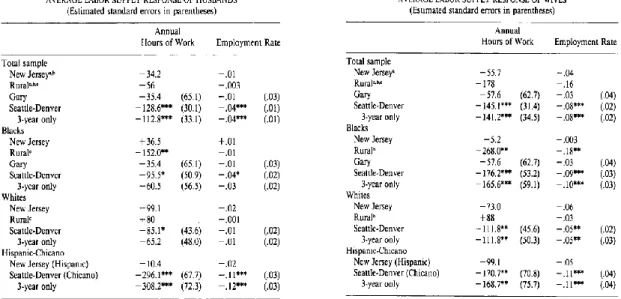
Despite being based on a different concept NIT experiments are able to shed some light on the behavior of lower income families in response to cash incentives. A first generic look can be taken at the average response of the 4 NIT experiments (Table 8, 9 and 10). Apart from husbands, all groups show a significant decrease in labor supply due to the incentive.
18 This type of behaviour is known as social desirability bias. People will tend to respond in a way that will be
seen as favorable by other. To see more: Foulsham & Kaminska (2013)
Source: Making the Difference – The BIG in Namibia (2009)
29
Moreover employment rates in these groups also present large reductions, meaning that people tend not only to work less but some even leave the labor market.
Table 8 - NIT- Husbands Labor Response Table 9 - NIT- Wives Labor Response
Table 10 - NIT- Single Female Heads Labor Response
These first numbers are noteworthy but given the heterogeneity of conditions in the 4 experiments let us have a deeper look on each of them individually. By looking at Table 2 we see that the New Jersey and the rural experiment were those whose criteria for eligibility were more tight (maximum income of 1.5 times the poverty line for a family of four). On the contrary, Gary and Seattle-Denver were more generous on this criteria allowing for households with income as high as 2.4 and 3.5 times the poverty line of four respectively to Source: Final Report of the Seattle-Denver Income Maintenance Experiment – Volume 1 (1983)
30
participate. Moreover the Seattle-Denver experiment was also the most generous in terms of the amount distributed with the lowest guarantee being 95% of the poverty level, a number close to the highest amounts delivered in the other regions. Results tend to confirm theory. Seattle-Denver shows for all of the groups the highest reduction in hours worked and employment rates. The NIT experiments also tell us how different households tend to have different responses. Both wives and single female heads show significant reductions in labor supply and employment enrollment, with numbers as high as 16% for the latter. As we did for poverty we need to address this having the status quo at the time for women and career in mind. This can help explain the difference in the response of man and woman. This assumption is corroborated by the numbers in the rural area, where reductions are substantially higher, as one should expect from more conservative regions as rural Iowa or rural North Carolina where tradition would label men as the money makers and women as housewives. After analyzing more thoroughly the labour supply response in terms of hours worked, let us see in more detail how NIT affects employment based on an estimated model. Table 11 summarizes the results.
Table 11 - NIT Employment Response
Percentage of people entering employment decreases more than 30% on all categories. The same happens with the share of households who get unemployed, a number never below 7.9%. However when we look on a one year horizon results are slightly different. The number of entries into employment is still negatively affected - although the size of the impact is smaller- but the number of entries into non-employment is actually reduced by NIT for women. Context can once again help to explain this. Given the low female participation rate
Source: Source: Final Report of the Seattle-Denver Income Maintenance Experiment – Volume – 1 (1983)
31
in the labor market and the importance of the man figure as head of the house it is expectable that women who are involved in paid work do it not only for the income but for a personal preference for a professional career. Hence such a benefit does not provide a disincentive high enough to quit their job. Finally the benefit also affects the length of both employment and unemployment. The first tends to be reduced by 15% on average and the latter increases by at least 42.3%.
The above analysis is important in two ways: first it tell us how real experiments show somewhat more sucessful results than those predicted by theoretical models. Second they allows us to make the bridge to the portuguese reality and understand what can and cannot be compared. We have seen that in the under-developed regions the incentive brought motivating results in terms of economic conditions. People were able to avoid deep scarceness and transform the incentive into something that allows them to become self-sustainable. Moreover labor supply responses tend to show no disincentive in terms of hours at work or participation in the labor market. Although we witness cases of severe deprivation in Portugal, the country’s reality is still very different. In Namibia and India we are dealing with a very primitive economy based mostly on the primary and secondary sectors. The challenges that people receiving the benefit in these regions face are somehow different and perhaps less demanding than those faced by potential beneficiaries in Portugal, specially in terms of inclusion. One would expect that in an economy that is eager for qualified workforce and where tecnhology and expertise are driving forces it is harder for people to become valuable for society. Nevertheless the type of temptations and potential disincentives that such a stimulus can bring to the population covered are fairly similar and one should not disregard the evidence brought by these experiments on these issues. As for developed regions, conclusions are a little different. In Alaska we saw that the dividend is indeed capable of recuding the incidence of poverty. However and mainly due to the small amount distributed, the measure has not been capable to avoid poverty rates to grow over the last decades, following the trend in the entire country. NIT experiments confirm what is perhaps the biggest concern regarding BI –labor supply response. This response seems to be highly sensitive to the generosity of the programme. We saw that the most generous schemes presented the most upsetting results regarding labor supply reduction. The results are also displeasing in terms of employment with reductions both in the probability of being employed and the time spent on a job and an increase in the chances of being unemployed and the time spent without a job. Since we will be dealing with people whose economic and social
32
situation is very related to those treated by the NIT, the analysis of both current and potential benefit’s size and generosity and its repercussions are of the essence in this work.
With these results in mind I will now move on to the next stage where I shall compare them with the results of the current Minimum Income Scheme in Portugal
33
4. Minimum Income Scheme vs Basic Income – A Portuguese Case
What I intend to do over this chapter is to look at the current state of the Portuguese Minimum Income Scheme and compare it with what we learnt so far about BI. As I stated earlier the focus of the analysis shall be on the Portuguese economy. Hence, when appropriate, several indicators will be examined in order to give useful context. In order to have a deeper grasp of the Portuguese scheme I am going to start with a small introduction explaining the main goals of the policy as well as its characteristics and origins. After this I will provide the usual analysis by topic starting with a look on poverty and then moving on to the subject of labor market.
4.1 Introduction –
The Portuguese GMI is a non-contributory benefit paid by the Social Security System. It was first introduced in 1996 under the name of Rendimento Minimo Garantido with the aim of ensuring households at risk the resources to satisfy basic needs and social and professional inclusion. The benefit is delivered according to the gap between the household income and a certain threshold defined by the state and is intended to close this gap. Changing the name to
Rendimento Social de Inserção (RSI) in 2003 – in line with the new focus of these type of
schemes regarding inclusion - the programme’s objective is not only to provide a minimum level of dignity to its beneficiaries but also to promote social integration through a job, vocational training or community service.
To better understand the size of the programme and its evolution we can look at Graph 8 and Graph 9. The graphs show us that each beneficiary receives around 110€, an amount that has been increasing over the last decade. On the other hand the number of beneficiaries has been dropping and is currently around 300.000. The total amount spent on this programme has also been decreasing since its implementation with a little turn over the last two years. RSI accounts for barely 1% of the total amount spent with social security, a sum that is around 300M€.
34
Graph 8 - RSI Evolution – Individuals vs Amount
Graph 9 - RSI as % of Social Security Expenditure
According to Statistics Portugal (INE), in 2015 the annual value that defined the poverty line in Portugal was 5268€. This corresponds to an average monthly value of 439€. Given that on average each beneficiary obtains 110€, this corresponds to about 20% of the poverty line income. Moreover the median net income in Portugal in 2015 was 8780€ (INE). Thus a benefit of 110€ represents around 12% of this average net income. These percentages are in accordance to those of the Alaska Dividend, although as we know in the Alaskan case the
287 110,90 0 20 40 60 80 100 120 0 100 200 300 400 500 600 2004 2006 2008 2010 2012 2014 2016 Individuals -Left Axis (Thousands of People) Value per individual -Right Axis
Source: Social Security Portugal(2017)
Source: Rendimento Minimo em Portugal – Retratos de 20 anos a desafiar práticas e (pre)conceitos ; Minimum Income in Portugal – a 20 year Portrait of challenges and pre(concepts)
35
benefit is universal. However when we compare to the amounts distributed in the other three experiments we see that the Portuguese scheme’s amount falls way below. The population targeted is more or less similar - those who are in the bottom deciles - with the obvious differences that exist between a nation as Portugal and the underdeveloped regions of Otjivero and Madhya Pradesh. This target is confirmed by the data. According to INE, the percentage of people at risk of poverty after social transfers is 19%19. This means roughly 2M citizens. With the programme targeting only 300.000 it is clear that the policy does indeed target those who are in the most severe situations leaving behind a large share of poor people. Lastly and given the relevance of the labor market topic for this work I believe that as an introductory note it is relevant to see how the RSI population compares with the country’s population in terms of work situation. Table 12 compares nationwide indicators with an RSI sample. The key figure is the difference in the share of unemployed people. With 60% of beneficiaries being unemployed, active market labor policies have to be taken into account when discussing the importance of a Minimum Income scheme. This discussion should take into consideration the results earlier found for the BI experiments namely how those in the bottom deciles behave in the presence of this kind of incentive
Table 12 - RSI Sample vs Portugal - Employment Data
After this short description, it is now interesting to look at the performance of the system in the context of the Portuguese economy and compare it to the results that were found on the Basic Income trials here examined. Several papers and reports have looked on the subject of RSI and its impact and I should refer to them on assessing the scheme. For this analysis I will look at the usual two main topics: Poverty and Labor Market.
19 The at-risk-of-poverty rate here described corresponds to an annual net income below €5,268 in 2015 (INE)
Portugal RSI sample
Active 60,2 75,3
Employed 49,6 14,6
Unemployed 10,6 60,7
Inactive 39,8 24,7
Source: Impactos dos Acordos de Inserçãono Desempenho do RSI(entre 2006-2009) -
DINÂMIA’CET; Impact of inlcusion Agreements in RSI performance (2006-2009); Statistics Portugal
36
4.2 Poverty –
The Portuguese Social Security describes RSI as a measure that is mainly intended to intervene in the most severe cases of poverty by protecting and supporting those who are facing a situation of deep scarceness20. Over the next lines we should see how successful has the measure been on achieving this and how different could a BI behave given the current Portuguese situation in this subject.
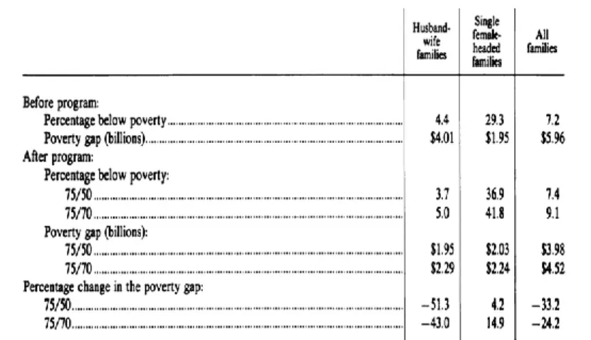
Existing data on this topic covers two periods, before and after a scheme reform in 2010. This reform changed the means-tested conditions, reducing substantially the number of beneficiaries. For this reason I shall do a comparative analysis rather than a single one. This will allow us to not only evaluate the scheme performance on alleviating poverty but also understand how the reform impacted the numbers. Table 13 shows us that RSI is being successful in lightening the severity and intensity of poverty with interesting numbers for both periods. The decrease on poverty incidence is minor and close to zero after the reform.
The country’s indicators on this topic are upsetting. Graph 10 shows the evolution of at-poverty-risk rates since 2004 in Portugal. We can see that we still face high rates and that those rates are not improving. These numbers are quite similar to those we saw for Alaska. The dividend in Alaska is not being able to stop the rise in the state’s poverty rates over the last years. The same is true for RSI in Portugal. The amount of the two transfers is also very equivalent. This means that even a universal income if not high enough cannot by itself tackle poverty. However the Alaskan benefit seems to achieve better results than the Portuguese one. In Alaska over the last decades the poverty rate never decreased on average by less than 2%.
20 Source: <http://www.seg-social.pt/rendimento-social-de-insercao> viewed at 3 March 2017
Source: Farinha Rodrigues (2012)
Table 13 - RSI Effects on Poverty
Note: After RSI(1) – Before the Reform; After RSI (2) – After the Reform
37
In Portugal even before the reform of the policy, RSI was only able to achieve a reduction of 0.3%.
Graph 10 - Poverty Evolution in Portugal
The country performs much better regarding the impact on the intensity of poverty. RSI seems able to reduce both intensity and severity by a number close to 1% in absolute value. Farinha Rodrigues (2012) calculates that 2.5% of the population is severely poor. This means roughly 250.000 people. Although the characteristics that define this type of severe poverty are different from those we observe in the under-developed regions21 analyzed in this work it is true that BI seems more effective in tackling them. In Namibia the number of people who were under the food poverty line dropped by 56% in absolute value. The best indicator available in Madhya Pradesh, number of children underweight, also enjoyed an interesting reduction of 19.5% in absolute value. Backgrounds are different and so are the conditions. The BI experiments were conducted with relatively small samples and had the clear aim of alleviating scarcity of those receiving the benefit. RSI is only one instrument in the Portuguese set of tools available to act on reducing poverty. Nevertheless the scale of reduction in terms of poverty severity is so high in the regions here observed that I believe that it is worth looking carefully at how beneficial a BI could be in improving these numbers in Portugal.
Looking now at efficiency, Table 14 shows us several measures that can help us with this analysis. The 2010 Reform had no significant impact on both the Vertical Efficiency of the
21 The European Comission defines severe poverty as not being able to purchase at least four of the nine
following items: to pay their rent, mortgage or utility bills; to keep their home adequately warm; to face unexpected expenses; to eat meat or proteins regularly; to go on holiday; a television set; a washing machine; a car; a telephone. 0 0,05 0,1 0,15 0,2 0,25 0,3 0,35 0,4 04 05 06 07 08 09 10 11 12 13
Poverty Evolution in Portugal
Mean Poverty Gap
Poverty Rate
38
Programme (VEP) and the Poverty Reduction Efficiency (PRE). The two indicators show really high numbers for both periods with minor improvements reflecting the tightening of rules. This means two things. First, it confirms that RSI is a measure only available to those in need. Such a high value of VEP means that nearly no beneficiary received the transfer without being poor. Second, the numbers for PRE show that the transfer although small is almost entirely devoted to reducing poverty. On the other hand the Poverty Gap Efficiency (PGE) presents less thrilling numbers. This measure which is an indicator of horizontal efficiency had a value of 27.3%, a number that dropped by half after the 2010 reform. Hence, by now RSI reduces the proportion of the aggregate poverty gap by only 15.4%. In the NIT experiments an estimate was made on the average poverty gap change by type of household. When we looked to families as a whole, the poverty gap reduction was over 24% for both of the scheme’s designs. The only situation where the individual would on average be worse off was for the case of single-female headed families. We saw before how these results could partially be explained by the status quo existent at the time in terms of participation of females in the labor market. Thus there is no reason to believe that better results would not be achieved.
Table 14 - RSI Efficiency Indicators
Another important issue debated while analyzing the impact of BI on poverty was its ability to increase the income that beneficiaries generate by its own efforts. For both Madhya Pradesh and Otjivero, the regions with available data on this, there was on average an increase on the income self-generated. To see how RSI behaves on this variable let us analyze the share of contracts that were terminated due to a change in income. Table 15 demonstrates that half of contracts terminated are so due to a change in the beneficiaries’ income. This should be seen as good news. However when we look at the same table we see that not even 1% are terminated due to integration in the labor market. This means that that income change is mostly conducted by other sources of income such as other social benefits or revenue generated by potentially unproductive activities that do not contribute effectively to promote
39
integration in society. Thus we see that RSI is not able to improve one’s ability to become more productive and hence self-sustainable.
Table 15 - RSI Contracts Terminated by Motive
When I first cross-examined what literature exhausts as the main differences between the effects of BI and Minimum Income on poverty we saw that the main point was the breakdown of the poverty trap provided by the introduction of BI. Minimum Income had the ability of avoiding beneficiaries from falling below a certain threshold that the state defines as a minimum for a decent living. However and mostly due to a marginal tax rate of 100% the measure was only half effective since it trapped the population covered in a cycle of “reasonable”poverty. The results we saw for Portugal confirm exactly this point. The scheme is successful in preventing the most severe types of poverty but it does not really affect its general incidence. Moreover it does not seem able to provide the necessary tools to avoid beneficiaries from becoming welfare dependent. BI on its turn showed more exciting results in fighting both poverty incidence and severity. For the case of under-developed regions it undeniably reduced scarceness and provided the means to prevent people from becoming trapped to the benefit. The boost in self-earned income is a sign of this. For the US experiments, although unable to stop poverty growth, BI was able to reduce much more effectively the incidence of it in Alaska, a region whose reality is fairly similar to Portugal. Source: Social security Portugal(2017)
40
4.3 Labor Market –
One of the RSI fundamentals is to promote an active inclusion of its beneficiaries in society. Active labor market policies are essential to achieve this. Thus, to evaluate the effectiveness and potential of the scheme it is vital to understand how successful it has been on promoting this inclusion. Over this chapter we will look at some of the indicators that describe the impact of RSI in the labor market. Furthermore and similarly to what I did in the previous chapter I will compare those effects to those observed in the BI experiments.
Let me start this analysis by comparing how different is the labor supply response produced by the two schemes. The data available on RSI does not report the changes in terms of hours or days worked. However I believe some interpretation can be made through several other indicators. As we saw earlier the unemployment rate amongst those who are under RSI is much higher than the national average (60.7% vs 10.6%). This shows how important it is to effectively promote inclusion with the scheme. Yet the number of people whose contracts were ceased due to finding a job is almost insignificant (Table 14). The number was never above 300 people, which represents a share of 1% or less from all the contracts terminated. Unable to act on those who are unemployed let us now see how does it affect those who are working. Tables 16 and 17 show that from the initial small share of people who were working – 8.1% of those interviewed and 26.5% of their spouses – around 40% became unemployed. In the case of the interviewees, only 39.4% of people kept working, a number that is lower than the one we find for spouses, 57.5%.
Table 16 - % of RSI Beneficiaries working - When claimed vs Now
Interviewee Spouse
Then Now Then Now
8,1% 8,6% 26,5% 25,2%
Source: Impactos dos Acordos de Inserçãono Desempenho do RSI(entre 2006-2009) -
DINÂMIA’CET; Impact of inlcusion Agreements in RSI performance (2006-2009); Statistics Portugal-