Universidade de Lisboa
Faculdade de Ciências
Departamento de Informática
Signatures of natural selection in the adaptive
immune system of primates
Bruno Eduardo Vasques Costa
Dissertação
Mestrado em Bioinformática e Biologia Computacional
Especialização em Biologia Computacional 2015
Dissertação
Mestrado em Bioinformática e Biologia Computacional
Especialização em Biologia Computacional
2015
Universidade de Lisboa
Faculdade de Ciências
Departamento de Informática
Signatures of natural selection in the adaptive
immune system of primates
Orientador:
Prof. Doutor Octávio Fernando de Sousa Salgueiro Godinho Paulo (FCUL) Prof. Doutora Hélia Cristina de Oliveira Neves (FMUL)
A presente dissertação foi escrita na língua inglesa, de forma a facilitar o processo de publicação de resultados sendo que esta é a língua oficial de disseminação de conhecimento pela comunidade científica.
Gostaria de agradecer ao Professor Doutor Octávio Paulo, à Professora Doutora Hélia Neves e à Professora Doutora Rita Zilhão, por me terem orientado durante este longo percurso. Agradecendo ao Professor Octávio pela frescura de abordagens a cada problema que surgia na construção desta tese, dando um apoio valioso para me apontar no caminho certo com otimíssimo, entusiasmo e segurança que o trabalho que estava a realizar tinha valor. Às Professoras Rita e Hélia pelo apoio que me deram a entender os fundamentos teóricos adjacentes ao trabalho prático, integrando-me no seu grupo de trabalho. Onde todas as semanas eram apresentados trabalhos com genes envolvidos na minha tese que me deram uma visão ampliada sobre o trabalho laboratorial relativamente ao trabalho in sílica. Todos este processos contribuíram enormemente para a minha evolução como cientista.
Quero agradecer à minha namorada:
- Raquel, muito obrigado pelo incentivo e apoio moral em momentos de dúvida deste longo processo de escrita, que não foi fácil.
Aos meus pais por acreditarem em mim e me darem o apoio necessário para realizar esta tese.
Aos colegas do CoBiG2 pelo imenso e constante incentivo e resposta às minha
dúvidas.
Ao Francisco pela paciência contínua, por me ensinar a trabalhar com um novo sistema operativo, me fornecer as bases para aprender a trabalhar em linha de comandos e apoio em imensas outras dúvidas técnicas, um amigo sempre disposto a ajudar. E à Joana e à Telma pela ajuda valiosa na análise dos resultados. Graças a vocês consegui exprimir com maior clareza as ideias expostas neste trabalho. Revelaram-se grandes amigas ao longo dos bons e especialmente nos maus momentos.
O desenvolvimento de uma resposta imunitária adaptativa possibilitou aos vertebrados montar uma defesa mais eficaz em resposta a agentes patogénicos. O sistema imunitário adaptativo tem a capacidade de reconhecer e guardar memória de agentes patogénicos específicos, conferindo ao sistema um poder de resposta mais rápido e eficaz aquando de uma reinfecção.
Com o sistema imunitário adaptativo surgem novas células, com o papel central na resposta imunitária. São exemplo dessas células, os linfócitos T e B, que produzem respectivamente os receptores das células T e B. Os receptores dos linfócitos T possuem grande capacidade de rearranjo das suas cadeias (α e β) e surgem de novo nos vertebrados mandibulados e em paralelo com o aparecimento dum novo órgão linfoide primário, o Timo. Este orgão é responsável pela maturação dos linfócitos T e tem a capacidade de eliminar linfócitos T autoreativos (isto é, que reconhecem o próprio).
Dada a importância do sistema imunitário adaptativo nos vertebrados, foi objectivo do presente estudo a analise bioinformática de um conjunto de 38 genes intimamente ligados ao desenvolvimento do sistema imunitário adaptativo. Estes, estão compreendidos no “processo de desenvolvimento do timo” e “processo do sistema imunitário”, e foram analisados em busca de assinaturas de seleção positiva, através da aplicação de modelos estatísticos (PAML), que estimam pelo método de máxima verosimilhança, o rácio (ω) de mutações não sinónimas (dN)
versus sinónimas (dS ) .
No presente estudo, em genes ortólogos, de 11 espécies de primatas (incluindo
Homo sapiens), encontraram-se sinais de seleção positiva em 7 genes que, após
estudos complementares, foram reduzidos a 4 genes: CD4, IFNG, HOXA3 e PTCRA. O mapeamento dos aminoácidos selecionados positivamente, por inferência Bayesiana, nas suas estruturas terciárias ou quaternárias, revelou que os aminoácidos selecionados positivamente se encontravam predominantemente na região de superfície, da respectiva proteína. Isto leva à formulação da hipótese, de que a superfície da proteína poderá estar sujeita a menores pressões seletivas purificantes do que o seu interior. Neste cenário, uma mutação terá menor impacto na conformação tridimensional, aquando do enrolamento da estrutura primária.
A ferramenta bioinformática SIFT, revelou que os aminoácidos selecionados positivamente surgem predominantemente em zonas putativamente menos conservadas.
Os resultados do presente estudo, sugerem que os genomas tidos como completos apresentam ainda zonas com baixa qualidade, ou baixa cobertura, que irão beneficiar grandemente da integração de reads produzidas pelos sequenciadores de 4ª geração, como a tecnologia Nanopore.
Palavras-Chave: Timo; Sistema imunitário adaptativo; PAML; Seleção Positiva;
The emergence of an adaptive immune response has enabled vertebrates to respond more effectively to pathogenic infection. The adaptive immune system has the ability to recognize and memorize specific pathogens, allowing stronger responses each time the pathogen is encountered. In the adaptive immune system, T and B-lymphoid cells are central players, producing T-cell and B-cell receptors, respectively. The T-lymphoid cells arise a second time in vertebrates in the jawed lineage. These cells display a more random recombination process of the α and β chains of their receptors, which is followed by coevolution of a primary lymphoid organ (thymus), essential for the development T-lymphoid cells, allowing the elimination of self-reacting cells.
Given the importance of the adaptive immune system in vertebrates, the present study aimed to analyze, from a bioinformatics perspective, a set of 38 genes annotated to “thymic development process” and “immune system process” GO terms. These genes were studied in order to find signatures of positive selection. To accomplish this, a statistical model (PAML) was applied to estimate the ratio (ω) of nonsynonymous (dN) versus synonymous substitutions (dS), through maximum
likelihood.
In the present study, in a set of orthologous genes, of 11 primate species (including
Homo sapiens), signals of positive selection were found in 4 genes: CD4, IFNG,
HOXA3 and PTCRA.
The amino acids identified with positive selection, through Bayesian inference, were mapped to their tertiary and quaternary structures, revealing that these were predominantly located on the protein surface. This leads to the formulation of the hypothesis that the protein surface is under lower purifying selective pressure than its core, with the consequent reduction of impact on the protein folding. The positively selected amino acids were mainly in regions putatively non-damaging or less conserved as predicted by the SIFT tool. This study brings to light problems in the so called complete genomes, that still bear regions of low quality, or low coverage, which will greatly benefit from fourth generation sequencing technology, like Nanopore.
Keywords: Thymus; Adaptive immune system; PAML; Positive selection;
1 NOTA PRÉVIA I 2 AGRADECIMENTOS II 3 RESUMO III 4 ABSTRACT V 5 TABLE OF CONTENTS 0 1 INTRODUCTION 1 1.1 GENERAL INTRODUCTION 1
1.2 IMMUNE SYSTEM AND HOW IT RESPONDS TO INFECTION 2
1.2.1 ADAPTIVE IMMUNE SYSTEM FUNCTION 2
1.2.2 CELLS IN THE ADAPTIVE IMMUNE SYSTEM 2
1.3 LYMPHOCYTE T DEVELOPMENT 4
1.3.1 THYMOCYTE MATURATION IN THE THYMUS 4
1.4 THYMUS ORGANOGENESIS 6
1.4.1 THYMUS DEVELOPMENT IN THE MOUSE MODEL AND IMPLIED GENES 7
1.4.2 COLONIZATION OF THE THYMUS BY LYMPHOID PROGENITOR CELLS 7
1.5 EMERGENCE OF THYMOPOIESIS IN VERTEBRATES 8
1.6 THE IMMUNE SYSTEM IN PRIMATES 8
1.7 PUBLIC DATABASES 8
1.8 EVOLUTION THROUGH MUTATION 10
1.8.1 DETECTION OF NATURAL SELECTION 10
1.8.2 DETERMINING THE OCCURRENCE OF NATURAL SELECTION 11
1.8.3 MICROEVOLUTIONARY METHODS 11
1.8.4 MACROEVOLUTIONARY METHODS 11
1.9 ESTIMATION OF SELECTION BY MAXIMUM LIKELIHOOD 13
1.9.1 SITE MODELS 13
1.9.2 THE BRANCH-SITE MODELS 14
1.10 OBJECTIVES 15
2 METHODS 16
2.1 COLLECTION AND SORTING OF GENE SEQUENCES FROM ENSEMBL 16
2.2 SELECTION OF THE SPECIES TO BE ANALYZED 16
2.3 GO TERM ENRICHMENT CLUSTERING 17
2.4 PREPARATION FOR ANALYSIS BY CODEML 17
2.5 DETECTION OF POSITIVE SELECTION 17
2.6 FUNCTIONAL ANALYSIS 18
2.7 CD4GENE SEQUENCE VALIDATION 18
3 RESULTS 19
3.1 GENES AND SPECIES SELECTION 19
3.2 GENE SELECTION 20
3.3 IFNG 21
3.3.1 FUNCTIONAL ANALYSIS 25
3.4.1 FUNCTIONAL ANALYSIS 30 3.5 HOXA3 31 3.6 FOXN1 33 3.7 GCM2 35 3.8 RUNX1T1 38 3.9 CD4 40 3.9.1 FUNCTIONAL ANALYSIS 45
3.9.2 VALIDATION OF CHIMPANZEE CD4 SEQUENCE 47
4 DISCUSSION 50 4.1 GENERAL DISCUSSION 50 4.2 IFNG 51 4.3 PTCRA 52 4.4 HOXA3 53 4.5 CD4 53 4.6 FINAL REMARKS 56 5 REFERENCES 57 6 APPENDIX 63
1.1 General introduction
The evolution from single cell organisms into multicellular organisms, could not have occurred without a mechanism that allowed unicellular organisms to distinguish between food and other unicellular organisms of its kind, or even another part of itself1,2. This is accomplished by one of the most basic functions of
the immune system: the ability to recognize specific surface receptors3.
With the evolution of ever more complex organisms, comes the need for a stronger immune response to infection. The emergence of the adaptive immune system must have been a game changer on the fight against pathogens, bringing the ability to recognize and remember specific pathogens, allowing stronger responses, each time the pathogen is encountered.
T-cells become central players in the immune system. The T-cell progenitors depend on the interaction with epithelial cells (thymic epithelial cells) of a lymphoid organ (thymus), in order to develop into mature functional antigen specific T-lymphocytes4.
Thus, the study of genes involved in the development of the adaptive immune system was indispensable to help provide answers to the question of how the adaptive immune system has been shaped in the last million years of evolution.
1.2 Immune system and how it responds to infection
The immune system is responsible for eliminating disease-causing microorganisms (pathogens), such as viruses, bacteria, fungi and parasites, and can be divided into innate and adaptive immune systems.
The innate immune system provides a nonspecific rapid general response that doesn’t improve with repeated exposure.
The adaptive immune system produces a slower, highly specific and long lasting response.
While both immune systems are capable of distinguishing between self and non-self, the innate system, has a limited number of receptors encoded from the germline, which are able to recognize common features in pathogens. Conversely, the adaptive immune system uses a process of somatic cell rearrangement to generate a wide repertoire of antigen receptors5.
1.2.1 Adaptive immune system function
The adaptive immune system comes into action, when the innate immune system alone, is incapable of dealing with an infection. Its major advantage over the innate immune system is its specificity, which allows a more targeted response against the pathogens and therefore is able to remove the threat with greater ease. This response produces antibodies (secreted by B-lymphocytes) and activated T-lymphocytes, which persist after the infection is eliminated and confer protection against reinfection6.
1.2.2 Cells in the adaptive immune system
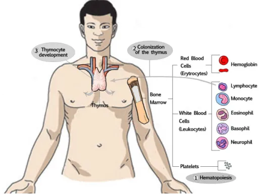
The main cells involved in the innate immune system, are granulocytes and dendritic cells, which originate from the bone marrow derived common myeloid progenitor. While in the adaptive immune system, the main cells are lymphocytes, derived from the common lymphoid progenitor. Both lineages are derived from bone marrowhematopoietic stem cells.
There are two types of lymphocytes, B lymphocytes (B cells) and T lymphocytes (T cells). The B cells proliferate and differentiate into antibody producing plasma cells when an antigen binds to its B-cell receptor (BCR).
Mature naïve T cells circulate between blood and peripheral lymphoid tissues, until they encounter their specific antigen7.This encounter induces the proliferation and
differentiation into effective T-cells (or activated). Activated T-cells differentiate into Cytotoxic, Helper or Regulatory effector T-cells depending on their cell markers.
Figure 1.2.1 - Main cells involved in the adaptive immune system.
In the peripheral lymphoid organ, the antigen (short peptide fragments of protein antigens) is presented by the major histocompatibility complex (MHC) on dendritic cells8 (host cell). MHCs are
transmembrane glycoproteins, that have a gap in the extracellular face of the molecule, where peptides can bind.
T-cells recognized the MHC presented antigen by the T-cell receptor (TCR). TCRs are membrane bound proteins, related to immunoglobulins, having both variable (V) and constant (C) regions. They are associated with an intracellular signaling complex.
The cytotoxic T cells express the CD8 and MHC (Class I) markers and kill infected cells that present its specific antigen. The cytotoxins (stored in specialized cytotoxic granules) released by CD8 cells can penetrate the lipid bilayer and trigger apoptosis in the target cell9.
Figure 1.2.3– Citotoxic T cell identifying an infected cell. Adapted from K. Murphy 2011
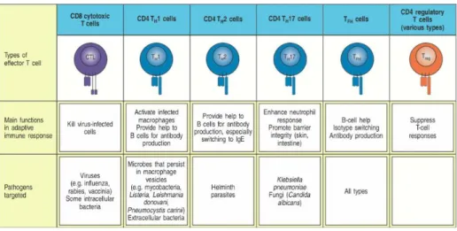
The Helper T cells (TH1, TH2, TH17, TFH) express the CD4 and MHC (Class II) markers
and activate their target cells, or Regulatory T cells, which help control the immune response10. This cellular communication is mainly mediated by cytokine molecules.
Figure 1.2.4 - Effector T cells and their respective function. Adapted from K. Murphy 2011. Figure 1.2.2 – Activation of a T cell by an antigen presenting dendritic cell. Adapted from K. Murphy 2011
Cytokines, are small soluble proteins that can alter the behavior or properties of the secreting cell or others11.
Figure 1.2.5 – Cytotoxins and cytokines produced by each effector T cell. Adapted from K. Murphy 2011.
The main cytokine produced by CD8 Cytotoxic T cells is interferon gamma (IFNG/IFN-γ), which can block viral replication or lead to the elimination of the virus from infected cells without causing their death. CD4 TH1 also secretes IFNG in
order to active macrophages that weren’t able to destroy ingested pathogens and has become incapacitated12,13.
1.3 Lymphocyte T development
All lymphocytes derive form bone marrow hematopoietic progenitor cells however T-lymphocyte differentiation (lymphopoiesis) takes place in another lymphoid organ. T cell differentiation depends on the interaction of hematopoietic progenitors and immature T-lymphocytes (thymocytes) with the thymic epithelium, which shapes the mature repertoire of T cells in order to ensure self-tolerance.
1.3.1 Thymocyte maturation in the thymus
T-cell development depends on cell-cell interactions, between the thymocytes and the thymic epithelial cells, which are critical for the complete morphological and functional maturation of both cell compartments14,, and determine thymocyte cell fate. If lymphoid progenitors at the T-cell/B-cell branch point received NOTCH1 signaling, these cells are prone to differentiate into T cells, whereas if presented with NOTCH2 the tendency is to differentiate to B-Cells15,16,17. Lymphocytes that
arrive at the thymus lack most cell markers characteristic of the T cells and their receptor genes aren’t rearranged yet. However through interaction with the thymic epithelium they start to differentiation towards the T cell lineage pathway.
There are two major populations of lymphocytes α:β and γ:δ. The rearrangement of the β and γ:δ chains determine the cell fate. Lymphocytes that have rearranged and express the γ:δ TCR shut off β chain rearrangement18. If injected in to peripheral circulation these cells can give rise to B cells.
Lymphocytes that complete β chain rearrangement, shut off γ:δ rearrangement and commit the cell to the α:β lineage.
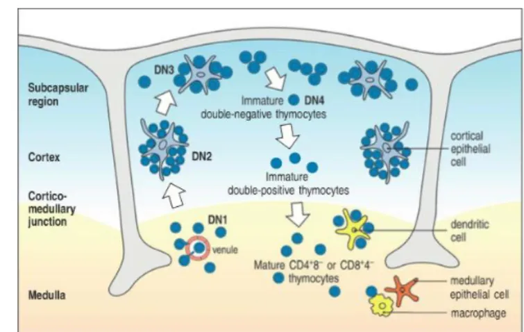
Thymocytes that go down the α:β pathway pass through various double negative (DN) stages based on the expression adhesion molecules CD44, CD25 and Kit.
DN1 – Both chains of the TCR are in the germline configuration.
DN2 – Rearrangement of β chain begins.
DN3 – Expressed β chains pair with a surrogate T-cell receptor α chain (pTα/PTCRA), and form a pre-TCR19. The pTα immunoglobulin domains makes two
important contacts that help with further rearrangement of the β chains. If β chain is incapable of pairing with the pTα the thymocytes is eliminated by apopthosis.
DN4 – Proliferation of cell with functional β chains.
Figure 1.3.1 – Thymocyte fate based on TCR chain and surface cell marker expression. Adapted from K. Murphy, 2011.
Figure 1.3.2 - Various phases of thymocyte development and surface marker expression timescale. In the Immunoglublin domain rearrangement, D stands for diverse genic segment, J for joining segment, V for variable segment and the subscript α/β refers to the chain.
Subsequently, the DN thymocytes, express CD8 and CD4 and becomes double positive (DP). While β chains in DP cells cease further rearrangement, the pTα begins a series of rearrangement attempts to produce an α:β TCR.
Afterwards, the α:β TCR are positively selected by compatibility with self-MHC molecules20. Self-reactive receptors are given a death signal, which leads to their removal though cell death (negative selection).
Thymocytes that survive selection cease expression, of one, of the co-receptor molecules. Therefore, becoming either CD4+CD8- or CD4 -CD8+ single positive (SP)
thymocytes, located in the medullar region that migrate to the periphery21,22.
Since defects in the thymic epithelium can result in immunodeficiency or autoimmunity. The expression of many tissue-specific self-antigens requires the autoimmune transcription factor regulator AIRE23. AIRE interacts with many
proteins involved in transcription, and is presumed to avoid termination of transcription from smaller promoter transcripts.
1.4 Thymus organogenesis
The thymus is composed by various lobules, and can be morphologically and functionally divided into an outer cortical region and an inner medulla. In young individuals, the thymus has a large number of developing T-cell precursors embedded in a network of epithelia. While in mature individuals, the development of new T cells in the thymus slows down, and numbers of these cells are maintained through long-lived individual T cells along with the division of mature T cells outside the central lymphoid organs.
Figure 1.4.1 - The cellular network of the human thymus. Adapted from K. Murphy, 2011.
Figure 1.3.3 - Thymocyte maturation through interaction with thymic epithelium. Adapted from K. Murphy, 2011.
1.4.1 Thymus development in the mouse model and implied genes
Thymic epithelium rudiment arises early during embryonic development, from endoderm-derived segmented structures, the pharyngeal pouches (PP).
In mammalian and avian embryos four PP are produced. However in avian embryos (chick and quail) the thymus and parathyroid glands are derived from the third and fourth PP 24, and thus
the thymus is formed from the third (3PP). Whereas in mammals, the thymus arises from a common primordium with parathyroid glands derived from the 3PP25. The formation of the 3PP
both in mouse, as well as, in chick and quail are dependent on the expression of HOXA3 gene26.
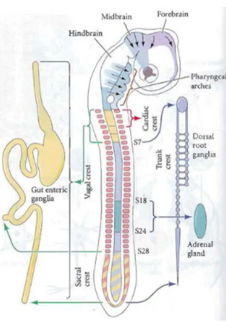
In mammals, the 3PP begins to outgrow surrounded by a condensed population of neural crest cells (NCC) that will lead to the formation of the thymic capsule27. Shortly after, segmentation
of the 3PP begins, though expression of GCM2 and FOXN1. GCM2 is responsible for the parathyroid28
cell differentiation while FOXN1 is responsible for the thymus differentiation29 Figure 1.4.2. FOXN1 is
the earliest known thymus-specific marker.
The proliferation of the epithelium leads to the stratified organization of the thymus. Once the 3PP is completely patterned into both thymus and parathyroid domains, the thymic primordia is separated from the pharynx and begins to migrate to its final anatomical position30.
These epithelial tissues form a rudimentary thymus, or thymic anlage that is ready to receive its first wave of thymocytes.
1.4.2 Colonization of the thymus by lymphoid progenitor cells
The colonization of the fetal thymus arises before its vascularization and occurs in two waves31,32. T cell
precursors respond to a gradient of chemokines33
(diffusible chemoattractant factors) that guide T-lymphoid progenitor cells out of the vasculature into the prevascular fetal thymus34. The second wave relies on
the expression of FOXN134 to keep the constant in-flow
of hemotopoietic precursors, into the thymus.
In the fetal primordium, thymic epithelial cells
produces transcripts for several chemokines, such as CXCL12, CCL25 and CCL2135. However, the CXC12, or its
Figure 1.4.2 - Regions of the chick neural crest. Adapted from S. Gilbert, 201099.
3PP
Figure 1.4.3 Segmentation of the third pharyngeal pouch by specific gene
expression. Adapted from C.
Blackburn, et al, 2004
Figure 1.4.4 - Migration of lympoid progenitor cell to the thymus.
receptor CXCR4, mutant mice, are still able to colonize the thymic anlage with T-precursor cells36. In CCR9-deficient (a receptor for CCL25) mice, a threefold
decrease in total thymocyte cellularity is exhibited when compared with wildtype animals37. Conversely, CCL21- and CCR7-deficient mice revealed that CCL21 is
involved in the colonization of the prevascular fetal thymus38.
Once the fetal thymus is fully vascularized, lymphocyte-progenitor cells have direct access to the thymus, via newly sprouted blood vessels39, where integrins and CD44
are suggested to play a role in thymus seeding 40.
1.5 Emergence of thymopoiesis in Vertebrates
The adaptive immune system has only been documented in vertebrates and it has been shown to evolve independently in two basal vertebrates: the lineage that gave rise to jawless vertebrates, such as hagfish and lamprey, and the lineage that gave rise to all jawed vertebrates, represented by cartilaginous fishes41.
While jawless vertebrates have lymphocytes with combinatorial diversity achieved through gene conversion, they still don’t have an adaptive immune system. In jawed vertebrates, combinatorial diversity is achieved by VDJ recombination. Thus, the thymus emerges in the jawed lineage involved in the self-reactivity process, which would be problematic due to the diversity generated by VDJ recombination42.
1.6 The immune system in primates
The immune system of nonhuman primates (NHP), shares a significant amount of homologous genes with the immune system of humans. The adaptive immune system of NHP species has been highly studied throughout the last decades and despite the similarity between species, the understanding of T cell repertoire dynamics is reduced. This is due to the lack of specific antibodies against human variable TCR and even less that cross-react with rhesus TCR43.
The varieties of pathogens that invade NHP are generally similar to human, and therefore differences in the immune response can be investigated44.
The study of genomic data of NHP will provide further insights into the immune system.
The high similarity and outbred nature of primates provides a great study model for further analysis of the adaptive immune function in order to provide new advances in the medical field45.
1.7 Public Databases
Public databases of scientific data are becoming key tools for research in biology, especially in the field of bioinformatics, being essential for worldwide spread of information. Nowadays, bioinformaticians have a wide variety of public databases at their disposal: from nucleotide sequence databases, like GenBank46, to whole genome databases, such as Ensembl47. There are also manually curated protein sequence databases, such as Swiss-Prot48, or it's automatic counterpart – Uni-Prot, and even metabolic pathway and functional databases like KEGG49 and many others. There are three major worldwide molecular biology databases, the US National
European Bioinformatics Institute (EBI) located in Hinxton, Cambridge UK, which is a
part of the European Molecular Biology Laboratory (EMBL) and the DNA Database of
Japan (DDBJ) operated by the Center for Information Biology (CIB) in Mishima, Japan.
NCBI, EBI and CIB comprise the International Nucleotide Sequence Database
Collaboration and synchronize their databases every 24h.
One of the best-known nucleotide sequence databases available at NCBI is GenBank. This database allows the query of billions of sequences and scientists can easily submit sequences to this database in order to accurately cite them in their publications though a unique record called accession number. NCBI uses the Entrez50
system to allow users to query all NCBI associated databases and implements logical operators in queries. Another fundamental bioinformatics tool provided by the NCBI is the Basic Local Alignment Search Tool (BLAST)51, which allows the calculation of
sequence similarities, enabling the comparison of nucleotide and protein sequences to those available in entire databases.
Amongst the constant evolution of sequencing technology throughout the 90s due to the human genome project, the implementation of pyrosequencing in sequencing technology and its widespread to major laboratories lead to the passage from genetics to genomics. However, genomic sequencing technology became affordable due to the appearance of new companies in the sequencing market caused by the mass sequencing.
In 1999 the Ensembl project which is a joint project between EBI, and the Wellcome
Trust Sanger Institute (WTSI) begins. Its mission is to provide automatically
annotated genomes integrated with other available biological data.
The Ensembl 76 release is the latest available as of August 2014 and comprises a list of 79 species, all of which have their genome publicly available.
Subsequently, with the completion of the human genome sequence, in order to discover all crucial parts of the human genome biological function. The Encyclopedia
Of DNA Elements (ENCODE)52, a public research consortium was launched in
September 2003 by the National Human Genome Research Institute (NHGRI), in September 2003.
1.8 Evolution through mutation
Natural selection is one of the major evolutionary forces responsible for the diversity of organisms, making it one of the most important processes in biology. Identifying its action on the molecular basics, has become a current question and several statistical methods have been created to look for the “molecular footprints” left by Selection in genomes and protein sequences.
Molecular adaptation occurs due to the action of evolutionary forces of mutation, migration, natural selection, and genetic drift, which affect the allelic frequencies in a population. When a mutation arises, a new genetic variant appears in the populational genetic background. If it is advantageous it may become widespread and eventually fixate (positive selection). However since random mutations are typically deleterious, there is a constant purifying selection (negative selection) acting on mutations in order to remove them from the gene pool.
Besides positive and negative selection, balancing selection also acts to preserve multiple genetic variants within a population, for very long periods of time. In diploids, balancing selection53 can be caused by overdominance, when the
heterozygote at a particular locus is associated with greater fitness than both the homozygotes, thereby maintaining both alleles54. Alternatively, both haploids and
diploids may display frequency-dependent selection, another form of balancing selection that occurs when a rare variant is associated with greater fitness than a more common one. Lastly, frequent environmental fluctuations, allow for multiple variants to be maintained since no single advantageous mutation has enough time to reach fixation, before the environment within which it is beneficial changes once again (fluctuating selection)55.
1.8.1 Detection of natural selection
Molecular sequences encompass different types of information that can be used, individually or in combination, to infer the past action of selection56.
The frequency of observed polymorphisms, depends on the action of
selection and drift at a particular site. Deleterious mutations are more likely to be found at low frequencies since they are typically negatively selected, before they become widespread. Mutations that have become fixed are much more likely to represent neutral or beneficial changes57.
The relative rate of silent and replacement fixations.
Non-synonymous nucleotide mutations are those that change the encoded amino acid, while Synonymous mutations maintain the coded amino acid unchanged, due to the redundancy inherent in the genetic code. A greater rate of fixation for Non-synonymous mutation, relative to the rate of Synonymous mutation, can be explained by action of positive selection.
Differences in genetic variation among genomic loci or among
populations.
Fixation of a mutation by positive selection leads both to loss of genetic variation at the selected locus, but also at genetically linked loci that may be
evolving neutrally. Hence, the pattern of genetic variability among genomic loci can be used to infer selection in a recombining population. Similarly, differences in genetic variation at the same loci in different populations can also indicate action of natural selection.
1.8.2 Determining the occurrence of natural selection
To detect signatures of natural selection there are two major methods employed to detect positive selection, macroevolutionary methods and microevolutionary methods in which summary statistic methods are frequently used, to compare the observed frequency of polymorphisms with the null hypothesis of selective neutrality. The summary statistic is the simplest way to investigate selection, using a sequence alignment. Statistics that summarize the relative frequency of polymorphic sites are calculated from the alignment, they are then compared with the values expected to occur under a “null model” of neutral evolution. If the observed statistics are significantly different from their expected values, then the neutral model can be rejected.
1.8.3 Microevolutionary methods
Microevolutionary methods, focus on population genetics to identify positive selection within species.
Tajima’s D summarizes the distribution of site frequencies of polymorphic
sites.
Fay & Wu’s H uses an outgroup sequence, from a closely related population
or species to identify sites that have become fixed in the main study population.
1.8.4 Macroevolutionary methods
Macroevolutionary methods, which is the case of a method used in this study are used to identify past events of positive selection though comparative methods. Comparative methods use information of differences in genetic variation, among genomic loci, or among populations, frequently associated with the frequency of observed polymorphisms and the relative rate of synonymous and non-synonymous mutations.
McDonald-Kreitman test58 measures the amount of adaptive evolution within a
population by comparing it to an outgroup in order to distinguish fixations from polymorphisms. This is done by calculating the amount of polymorphisms in each species at neutral and non-neutral sites. A non-neutral site is one where the polymorphism is advantageous or deleterious, thus being prone to selection.
However, this test may be unreliable due to underestimation of degree of selection in presence of slightly deleterious mutations59.
DN/dS60 methods, concentrate on the relative rate of synonymous and non-synonymous mutations61 and is the method used to analyze the data in this study.
DN/dS methods, classify mutations in coding sequences as either synonymous or
non-synonymous. Assuming that selection acts less strongly on silent mutations, observed differences between patterns of synonymous and non-synonymous mutations should reflect the action of natural selection.
If all non-synonymous mutations are neutral then, by definition the ratio of the two rates must equal one, indicating no selection.
DN and dS are calculated for every non-synonymous or synonymous site, taking into
account the fact that random mutations generate more non-synonymous than synonymous mutations, due to the nature of the genetic code62. If the ratio is
significantly greater than one, then positive selection is the most plausible scenario. dN/dS methods are most successful in detecting adaptation when applied to genes
that are under antagonistic co-evolution events, such as those generated by sexual conflict, predator-prey interactions, or host-parasite interactions63.
However, this method is statistically weak and may fail to detect many instances of selection64. Notwithstanding, unlike the summary statistics introduced before, dN/dS
methods do not require strong assumptions about the sampled population, and are therefore considered to be more robust.
1.9 Estimation of selection by maximum likelihood
The summary statistic (ω), which is a gene-based method is recurrently used to detect positive selection. One of the most used tools to calculate these ratio is PAML65.
PAML is a Phylogenetic Analysis by Maximum Likelihood software that uses phylogenetic methods to preform comparative analysis of DNA and protein sequences by maximum likelihood. These phylogenetic methods are useful to estimate the evolutionary rates of genes and genomes, and to detect footprints of natural selection.
CODEML, a module of PAML, preforms comparisons and tests of phylogenetic trees by estimating parameters in sophisticated substitution models, including models for combined analysis of multiple genes. It estimates the synonymous (dS), and nonsynonymous (dN) substitution rates, permitting the detection of positive selection in protein-coding DNA sequences. To do this, CODEML uses to different methods: sites model, and branch site model.
1.9.1 Site models
The site models assume the same ω value for all branches. This method includes:
M0 (one ratio) ignores chemical differences between amino acids and uses the same nonsynonymous/synonymous rate ratio (ω=dN/dS) for all
nonsynonymous substitutions;
M1a (nearly neutral) assumes two site classes with ω0=0 and ω1=1, and does
not allow sites with ω>1;
M2a (selection) adds a third site class and allows the presence of positively selected sites66;
M3 (discrete) allows three site classes ω0, ω1 and ω2 that can take any value; M7 (beta) adopts a beta distribution for ω that is limited to the interval (0,1);
M8 (beta & ω) adds one more site class to M7, with ω ratio estimated from the data67.
For each model a log likelihood value is calculated by maximum likelihood . This value enables a comparison of an alternative model (positive selection allowed: H1)
to the nested statistical model (no positive selection allowed: H0), through a
likelihood ratio test (LRT). The LRT is calculated through twice the log likelihood of the difference between the two compared models (2Δ ). If H1 estimates ω>1 and the
LRT is greater than the critical values of the chi-square distribution with the appropriate degree of freedom (d.f.), then positive selection can be inferred. There are three pairs of models used to detect positive selection where a null model that doesn’t allow ω>1 is compared against a more general model that does:
H0: Uniform selection among sites (M0)
H1: Variable selective pressure among sites (M3)
H0: variable selective pressure but NO positive selection (M1) H1: variable selective pressure with positive selection (M2)
H0: Beta distributed variable selective pressure (M7) H1: Beta plus positive selection (M8)
When the likelihood ratio tests suggests positive selection, the Bayes empirical Bayes (BEB)68 method can be used to calculate the posterior probabilities of each
codon.
1.9.2 The branch-site models
The branch-site models assume different ω values among branches. This method includes different models to test particular lineages (foreground) for signals of positive selection:
Model 0, applies one ω for all branches and is mainly used for site models or as a
null hypotheses.
Model 1 (free ratios model), calculates separate ω for each branch in one run,
however this model uses a big number of parameters.
Model 2, allows the user to specify which branches to test for signals of positive
selection, only allow one branch to be tested per run. In model 2 there are two tests implemented to check for branch specific positive selection69, both of which
use model A as the alternative hypotheses:
Test 1, uses as a null hypothesis the site model M1a (nearly neutral) that
assumes two site classes with 0 < ω0 < 1 and ω1 = 1, this test however can be
misleading if relaxed selection acts on the foreground branch70.
Test 2, uses as a null hypotheses branch-site model A with ω2=1 fixed. This
allows sites evolving under negative selection on the background lineages to be released from constraint and to evolve neutrally on the foreground lineages.
Branch-site model A uses the parameters on Table 1.9.1.
By using test 2 it is possible to directly test weather a lineage evolves by positive selection if the null hypotheses is rejected based on the .
Table 1.9.1 - Branch sites Model A parameters
Site class Proportion Background Foreground
0 p0 ω0 =0 ω0=0
1 p1 ω1=1 ω0=1
2a (1-p0-p1)p0/(p0+p1) ω0=0 ω2 1
1.10 Objectives
The main objectives of this work, was to study a network of cellular development genes related with the adaptive immune system in primates. This approach may shed light on how primates have evolved to adapt to pathogens and disease, and shed light on which genes are evolving due to positive selection. To accomplish this, three main goals have been set:
Compilation of genetic data from public database for a large number of orthologous species, for a set of genes based on adaptive immune system development.
Analysis of the presence of selection among the lineages of species, recurring to the selected set of genes
2.1 Collection and sorting of gene sequences from Ensembl
The identification of genes linked to thymus tissue development, was performed by searching Gene Ontology database (http://amigo.geneontology.org), for the go terms “thymus”, “T cell” and “cytokine” in a list of 84 genes expressed by the QIAGEN Human Notch signaling pathway RT2 Profiler™ PCR Array. This search returned 24 genes, which were added to another 14 genes selected from the literature4,71,24. For
each gene its respective coding sequences were downloaded from the Ensembl database (http://www.ensembl.org - release 76 - 15/08/2014), though the Ensembl API. A Perl script (https://github.com/netbofia/ensembl_sequence_getter) was used for this purpose. Once the human coding sequences were found, a list of orthologous genes (from primate species) was selected and their respective coding sequences, downloaded.
2.2 Selection of the species to be analyzed
After some tests with different types of species the final dataset was constructed using 11 different species of primates Table 2.2.1.
Table 2.2.1 - List of primate species.
Primate List
Common name Scientific name Bushbaby Otolemur garnettii
Chimpanzee Pan troglodytes
Gibbon Nomascus leucogenys
Gorilla Gorilla gorilla
Human Homo Sapiens
Macaque Macaca mulatta
Marmoset Calithrix jacchus
Mouse Lemur Microcebus murunus
Olive baboon Papio anubis
Orangutan Pongo abelii
2.3 Go term enrichment clustering
All 38 human genes were blasted using “blastX” against the “nr” database using Blast2go. The most significant terms were complied and exported to SPSS to preform k-means clustering and hierarchical clustering.
The bioinformatics tool DAVID was used to obtain Go terms enrichment scores, and construct clusters.
2.4 Preparation for analysis by CODEML
All genes were filtered for primate species only and their transcripts were chosen based on size, using only one transcript per orthologous specie, where transcripts with a size difference, above 10%, from the chosen human transcript were excluded. All sequences were “blasted” using blastN against the “nt” database (accessed on 29/08/2014) to confirm their identity. Sequences were aligned with translatorX72
tool using MAFFT73 as the protein alignment method. The sequences were trimmed
for stop codons using in house python scripts. Maximum likelihood phylogenetic trees were calculated with RAxML74 using the GTRCAT model, with 1000
bootstrapped trees for each set of orthologous genes. The same process was conducted with Mr. Bayes to get the branch posterior probabilities.
All these methods were done by scripts, created specifically for this purpose (https://github.com/netbofia/paml_pipleline.git).
2.5 Detection of positive selection
CODEML from PAML 4.665 was used to test for positive selection. Firstly by applying
to each set of orthologues genes, the free ratio model (Model: 1) where each branch is able to evolve at different omega ratios based on their calculated phylogenetic trees. Genes with evidence of positive selection were further analyzed with a series of branch specific models: first the omega ratio of previously identified branches was tested individually by indicating with a “#1” the branch under study in each run (Model:2 Nssites:0) and evaluating the statistical value compared to the one-ratio model of sites model (M0) through a likelihood ratio test. Then to confirm the previous test, a branch site model A (Test 2), (Model:2 Nssites:2) which allows sites evolving under negative selection on the background, was used. Furthermore, the sites model (Model:0 NSsites: 0.1,2.3,7.8) with 3 site classes (ncat=3) for M3 and 10 site classes (ncat=10) for M8 were also applied to see the distribution of selection among sites, throughout the originating protein. The models M3 vs. M0, M2 vs. M1 and M8 vs. M7 were tested through likelihood ratio tests, with d.f.=5, d.f.=1 and d.f.=1 respectively. The results were collected by a python script that clustered the relevant calculated parameters (dn/ds, kappa, omegas, probabilities, posterior probabilities and log likelihood) for each model into a table in excel per gene, along with the then calculated likelihood ratio test and respective p-value for each pair of models. Branch site model results (tress with nodes) were extracted with tree searching algorithms construted in python. This algorithm is recursive and makes recursive calls to itself, spaning a new instance for each branch until it reaches a tip. The collected information is merged with the branch in order to create the phylogenetic trees and to detect which genes have branches with values that merit further study (https://github.com/netbofia/paml_pipleline.git).
2.6 Functional analysis
The positively selected sites in genes under evolution were plotted against the average sift score calculated for all possible amino acid transitions. The sift scores were calculated on the SIFT75 human protein webtool. The protein family domains
were identified by Pfam a protein family database from EMBL-EBI76.
The 3D human protein structures available were downloaded, for the protein sequences, in order to help in the visualization of the protein regions were the positively selected residues occurred. The protein structures were viewed using PyMol tool. When the protein structure wasn’t available it was calculated though homology modeling, using similar proteins as templates with SWISS-MODEL77.
2.7 CD4 Gene sequence validation
In order to confirm the chimpanzee sequence for CD4, the Ensembl chimpanzee mapped reads (.bam files) were downloaded from the Ensembl ftp server site. The chromosome 12 was extracted and visualized with samtools. Tables of nucleotide variation from the various reads were compiled using the BAM_to_TCS.py program from 4pipe4 tool (https://github.com/StuntsPT/4Pipe4, as of the commit
8ec3e53badbcdf97f940604095950686044edff7).
The CD4 sequence was confirmed by blasting the Ensembl exon9 sequence against the reads of the chimpanzee genome downloaded from the Washington University server
(http://genome.wustl.edu/pub/organism/Primates/Pan_troglodytes/assembly/). Then, to access their quality, its quality values were selected and surveyed using a in-house python script.
3.1 Genes and species selection
In this study 38 genes Table 3.1.1 involved in tissue development of the immune system were used, with a total of 9412 GO terms, 7830 GO terms for biological process, 940 GO terms for cellular component and 642 terms for molecular function Table 3.1.2.
Table 3.1.1 Gene list with full name.
Gene symbol Full name
ACKR2 Atypical Chemokine Binding Protein 2 ACKR3 Atypical Chemokine Receptor 3 Isoform x1
ADAM10 Disintegrin and Metalloproteinase Domain-containing protein 10 ADAM17 Disintegrin and metalloproteinase domain-containing protein 17
Aire Autoimmune regulator
CCL25 C-C motif chemokine 25 isoform 2 precursor CCR9 C-C chemokine receptor type 9 isoform x1
CD4 T-cell surface glycoprotein CD4 isoform 1 precursor
CD8 T-cell surface glycoprotein CD8 alpha chain isoform 2 precursor
CHUK Conserved helix-loop-helix ubiquitous kinase
CTNNB1 Catenin beta-1 isoform x1
CXCL12 Stromal cell-derived factor 1 isoform x3 CXCR4 Chemokine (c-x-c motif) receptor 4
DLL1 Delta-like protein 1
DLL4 Delta-like protein 4
DTX1 E3 ubiquitin-protein ligase dtx1
FOXN1 Forkhead box protein n1
GCM2 Chorion-specific transcription factor gcmb
HES1 Hairly Enhancer of Split-1
HOXA3 Homeobox protein hox-a3
HOXB4 Homeobox protein hox-b4
IFNG Interferon gamma
IL2RA Interleukin 2 alpha
IL6ST Interleukin 6 signal transducer ( oncostatin m receptor)
IL17B Interleukin 17b
JAG1 Jagged 1 (alagille syndrome)
JAG2 Jagged 2
LMO2 Rhombotin-2 isoform x1
NOTCH2 Neurogenic locus notch homolog protein 2 isoform 1 NOTCH4 Neurogenic locus notch homolog protein 4
NFKB1 Nuclear factor nf-kappa-b p105 subunit isoform x1 RUNX1 Runt-related transcription factor 1 isoform aml1b RUNX1T1 Protein cbfa2t1 isoform x3
PTCRA Pre t-cell antigen receptor alpha
PSEN1 Presenilin-1 isoform x1
PSEN2 Presenilin-2 isoform x1
SHH Sonic hedgehog homolog
3.2 Gene Selection
To detect genes, with accelerated evolutionary rates in the human specific branch the CODEML model 1 (Free ratio model) was applied to 38 genes off the 11 species of primates Table 2.2.1. From this, 7 genes revealed signals of positive selection - CD4, FOXN1, GCM2, HOXA3, IFNG, PTCRA and RUNX1T1 - that were further analyzed.
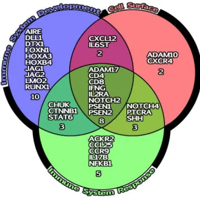
Figure 3.2.1 Venn diagram based on Go terms: Immune System response, Cell Surface and Immune system development.W
3.3 IFNG
(HGNC Symbol)
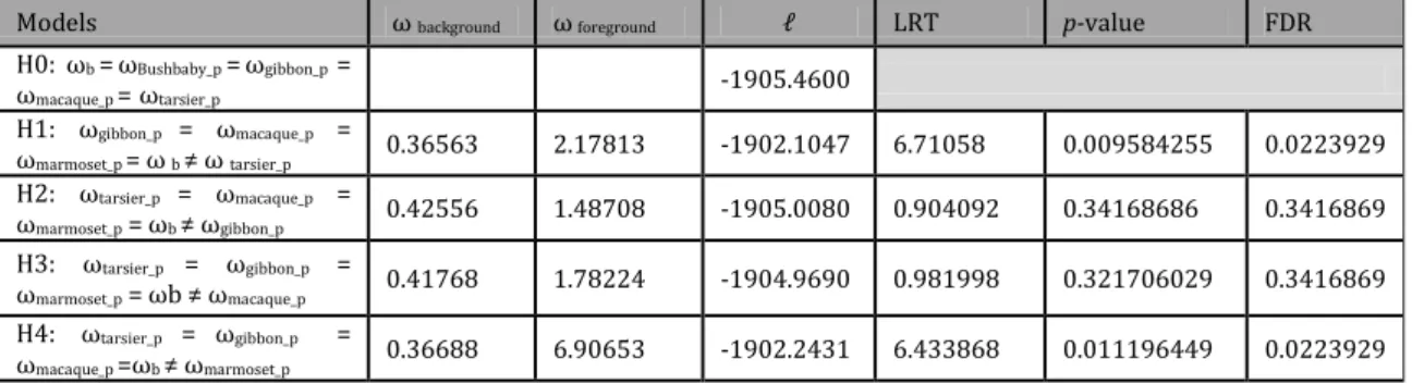
The free ratio model Figure 3.3.1 estimated that four branches are under positive selection, the Tarsier ancestral branch (Tarsier_p) with an ω ratio of 1.5703, the Marmoset ancestral branch (Marmoset_p) with an ω of 1.3478, the Gibbon ancestral branch (Gibbon_p) with an ω of 1.3092 and the macaque ancestral branch (macaque_p_p) with an ω of 1.4734.
Estimates were confirmed by testing each individual branch and preforming likelihood ratio tests, Table 3.3.1 both the Marsmoset_p (H4) and the Tarsier_p (H1) rejected the null hypothesis and estimate the omega ratio for the foreground branch at ω=2.17813 and 6.90653 respectively. While the Macaque_p and the Gibbon_p branch failed the likelihood ratio test.
The branch site model A Table 3.3.2 also followed the same pattern however upon correction of the values due to multiple testing the Tarsier_p p-value goes above 0.05 and fails the likelihood ratio test but has an ω ratio of 10.7596. The Marmoset_p branch has an estimate ω ratio of 27.57294. Both the Marmoset_p and the Tarsier_p branches detected positively selected sites though the BEB method both amino acid alignments of the positively selected site can be viewed in Figure 3.3.2 and Figure 3.3.3, respectively.
Figure 3.3.1 - Phylogenetic tree for gene IFNG with omega ratios on each node calculated by the free-ratio model in codeml. Bootsrtrap values calculated with RAxML and posterior probabilities calculated by Mr. Bayes are indicated on each branch respectively. Four branches that are under positive selection are indicated in red.
Table 3.3.1 - Parameter estimates under model of various omegas ratios among lineages and respective LRTs. LRT - Likelihood ratio test, FDR - False discovery rate correction, ωb background omega.ωf foreground omega.
Models ω background ω foreground LRT p-value FDR
H0: ωb =ωBushbaby_p =ωgibbon_p = ωmacaque_p = ωtarsier_p -1905.4600 H1: ωgibbon_p = ωmacaque_p = ωmarmoset_p = ω b ≠ ω tarsier_p 0.36563 2.17813 -1902.1047 6.71058 0.009584255 0.0223929 H2: ωtarsier_p = ωmacaque_p = ωmarmoset_p = ωb ≠ ωgibbon_p 0.42556 1.48708 -1905.0080 0.904092 0.34168686 0.3416869 H3: ωtarsier_p = ωgibbon_p = ωmarmoset_p = ωb ≠ ωmacaque_p 0.41768 1.78224 -1904.9690 0.981998 0.321706029 0.3416869 H4: ωtarsier_p = ωgibbon_p = ωmacaque_p =ωb ≠ ωmarmoset_p 0.36688 6.90653 -1902.2431 6.433868 0.011196449 0.0223929
Table 3.3.2 - Branch site Model A estimates for Tarsier_p, Marmoset_p, Gibbon_p and Macaque_p, branches. LRT - Likelihood Ratio Test, FDR - False Discovery Rate correction applied to p-values.
Model A ω background ω foreground LRT p-value FDR
H0: Tarsier_p 0.04568 1.00000 H0-1883.640034 4.5609 0.03 0.06 H1-1881.359572 H0: Giboon_p 0.13090 1.00000 H0-1884.533001 0.0451 0.83 0.83 H1-1884.510426 H0: Macaque_p 0.13208 1.00000 H0-1884.406791 0.0791 0.78 0.83 H1-1884.367253 H0: Marmoset_p 0.13409 1.00000 H0-1884.577027 7.0150 0.01 0.04 H1-1881.069509 H1: Tarsier_p H1:Giboon_p
Proportion ωbackground ω foreground Proportion ωbackground ω foreground
Class site 0 0.48785 0.1098 0.1098 Class site 2a 0 0.13095 0.13095
Class site 1 0.31379 1.00000 1.00000 Class site 2b 0 1.0000 1.00000
Class site 2a 0.12072 0.1098 10.7596 Class site 2a 0.58683 0.13095 1.35164
Class site 2b 0.07765 1.00000 10.7596 Class site 2b 0.41317 1.00000 1.35164
H1: Macaque_p H1: Marmoset_p
Proportion ωbackground ω foreground Proportion ωbackground ω foreground
Class site 0 0 0.13244 0.13244 Class site 0 0.56201 0.13731 0.13731
Class site 1 0 1.00000 1.00000 Class site 1 0.29625 1.00000 1.00000
Class site 2a 0.60068 0.13244 1.79372 Class site 2a 0.09281 0.13731 27.57294
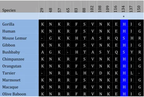
Species 29 48 57 65 83 88 102 108 109 116 134 137 150 * Gorilla K N K R F S V N K E H I G Human K N K R F S V N K E H I G Mouse Lemur - G K K H T A S R Q S H R Gibbon K N K R F S V N K E H I G Bushbaby A G K - H T A S Y Q S Y R Chimpanzee K N K R F S V N K E H I G Orangutan K N K R F S V N K E H I G Tarsier - N R R L H V D K K H L - Marmoset K N R R F S V N K E H I G Macaque K N R R F R V N K E H I G Olive Baboon K N R R F R V N K E H I G Species 28 29 31 33 68 81 83 90 101 110 112 113 121 127 137 141 146 149 150 166 * Gorilla_ENSGGOT00000006066 V K A N M K F Q N K R D Y N I A A T G Q Human_ENST00000229135 V K A N M K F Q N K R D Y N I A A T G Q Mouse_Lemu_ENSMICT00000004218 - - - - I E H K I S L E L Q H N R Q R K Gibbon_ENSNLET00000004455 V K A N M K F Q N K R D Y N I A A T G Q Bushbaby_ENSOGAT00000004301 S A I Q I E H K I S A E I Q Y V G L R K Chimpanzee_ENSPTRT00000009540 V K A N M K F Q N K R D Y N I A A T G Q Orangutan_ENSPPYT00000005616 V K A N M K F Q N K R D Y N I A A T G Q Tarsier_ENSTSYT00000001577 - - - - I E L K I D V E L Q L L R L - K Marmoset_ENSCJAT00000014072 V K A N M K F Q N R Q D Y N I A A I G Q Macaque_ENSMMUT00000027007 V K A N M K F Q N K R D Y N I A A I G Q Olive_babo_ENSPANT00000015498 V K A N M K F Q N K W D Y N I A A I G Q Figure 3.3.3 - Alignment of Amino acid residues with positive selection on the Tarsier ancestral lineage according to branch site model A BEB analysis. * 0.95 < p.p. <0.99 - ** p.p. >0.99
Site models analysis estimates that 1% of the amino acid sites, were under positive selection at an average ω ratio of 9.40 according to M3 and 8.25 according to M8 Table 3.3.3. The model M2a failed the likelihood ratio test. One amino acid residue with a posterior probability between 0.99 and 0.95 was detected and Figure 3.3.4. In order to visualize the distribution of the three classes identified by M3 a stacked histogram was plotted in Figure 6.0.2, where is possible to identify the selection sites.
Figure 3.3.2 - Alignment of Amino acid residues with positive selection on the Marmoset ancestral lineage according to branch site model A BEB analysis. * 0.95 < p.p. <0.99 - ** p.p. >0.99 .
Table 3.3.3 - Site model analysis, same omega for all branches, PPS – Positively selected sites, Likelihood, Likelihood ratio test, * 0.99 > p.p. >0.95 and ** p.p. > 0.99.
Model dn/ds kappa Parameters PSS lnL lnR p-Value
M0 (one ratio) 0.43 3.27 ω= 0.43 -1905.46 M1a(neutral) 0.49 3.45 p0= 0.59 p1= 0.41 -1885.51 ω0= 0.14 ω1= 1.00 M2a(selection) 0.58 3.60 p0= 0.57 p1= 0.42 p2= 0.01 2 *0 **0 -1882.71 5.597 0.0610 ω0= 0.14 ω1= 1.00 ω2= 9.65 M3(Discrete) 0.57 3.58 p0= 0.55 p1= 0.44 p2= 0.01 1 *1 **0 -1882.70 45.506 3.1205E-09 ω0= 0.13 ω1= 0.96 ω2= 9.40 M7 (beta) 0.47 3.39 P= 0.37 q= 0.42 -1885.94 M8(beta & ω) 0.55 3.52 p1= 0.01 ω= 8.25 5 *1 **0 -1882.74 6.390 0.0410 p0= 0.99 P= 0.39 q= 0.43 Species 112 * Gorilla R Human R Mouse_Lemur L Gibbon R Bushbaby A Chimpanzee R Orangutan R Tarsier V Marmoset Q Macaque R Olive_baboon W
Figure 3.3.4 - Alignment of Amino acid residues with positive selection M3 NEB analysis. * 0.95 < p.p. <0.99 - ** p.p. >0.99
3.3.1 Functional Analysis
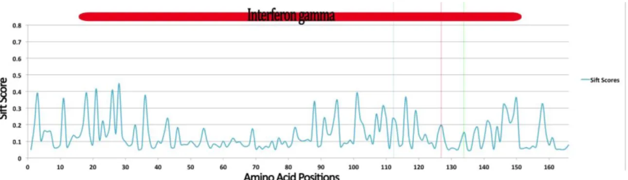
Sift scores for all the positions and the respective average of each position was calculated. Averages were used to plot the graph in Figure 3.3.5. Low sift score are associated to highly damaging (<0.1) mutations while higher scores are associated to tolerated mutations based on human protein structures78. Its possible to see the
highest positively selected residues identified earlier, represented in zones with tolerated mutations.
Figure 3.3.5 - Average sift score for each possible amino acid mutation throughout IFNG, with Pfam domain types positioned in red over graph and highest positively selected residues shown with colored vertical lines. Green line corresponds to the marmoset ancestral branch, red line corresponds to the tarsier ancestral branch and blue to the sites model M3 NEB posterior probability.
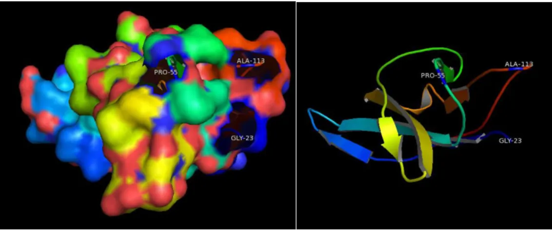
The tertiary structure was calculated by modeling the protein sequence to the 1eku.179 template of IFNG calculated by x-ray crystallography. The tertiary structure
Figure 3.3.6 shows that the selected residues were found on the protein surface region.
A B C
Figure 3.3.6 – IFNG tertiary structure with surface area rendered. A shows the a.a. residues HIS-134 and ASN-127 on the surface of the protein, B shows ARG-112 in region of the protein, C IFNG tertiary structure without surface area rendering
3.4 PTCRA
(HGNC Symbol)
The free ratio model estimated five branches Figure 3.4.1 to be evolving under positive selection: the Human ancestral branch (Human_p) with an omega ratio of 1.0704, the Gorilla branch with an omega ratio of 1.3474 the Macaque ancestral branch (Macaque_p) with an omega of 3.8731, the Gibbon branch with an omega ratio of 1.1572 and the Macaque branch with an omega ratio of 1.1621. Each branch was tested individually to correct for over estimation by the free ratio model. None of the tested branches passed the likelihood ratio test.
Besides that, testing the branch sites model A, Table 3.4.2 also suggests, that no particular branch has evolved though positive selection.
Nevertheless the site models Table 3.4.3 suggest that 31% of the amino acid residues evolved though positive selection had an average ω ratio of 1.81. An alignment of the amino acid residues, identified with positive selection though the NEB method, were plotted in Figure 6.0.2 and a stacked histogram with the distribution of the amino acids though the 3 class sites identified by M3 are represented in Figure 3.4.2, where it is possible to identify the selection sites.
Figure 3.4.1 - Phylogenetic tree for gene PTCRA with omega ratios on each node calculated by the free-ratio model in CODEML. Bootstrap values calculated with RAxML and posterior probabilities calculated by Mr. Bayes are indicated on each branch respectively. Five branches that are under positive selection are indicated in red.
0.0 GORILLA #1.3474 OLIVE_BABO #0.2332 BUSHBABY #0.4817 ORANGUTAN #0.3518 MARMOSET #0.3259 MACAQUE #1.1621 HUMAN #0.9017 CHIMPANZEE #0.7318 GIBBON #1.1572 #0.3021 #0.5902 #1.0704 #999.0000 #0.5304 #3.8731 97/1.0000 74/0.9907 81/0.9189 42/1.0000 100/1.0000 42/0.7648
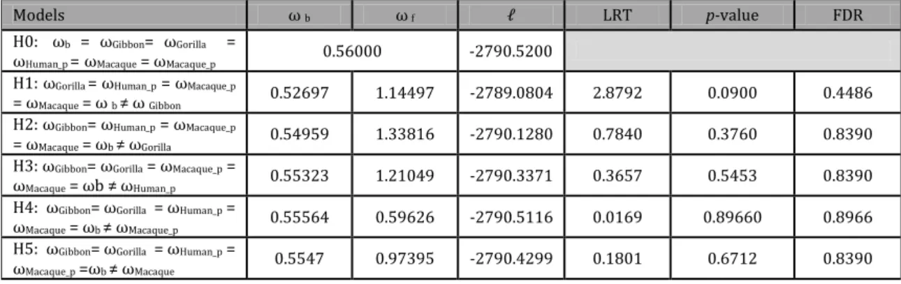
Table 3.4.1 - Parameter estimates under model of various omegas ratios among lineages and respective LRTs. LRT - Likelihood ratio test, FDR - False discovery rate correction, ωb background omega. ωf foreground omega.
Models ω b ω f LRT p-value FDR
H0: ωb = ωGibbon= ωGorilla =
ωHuman_p = ωMacaque = ωMacaque_p 0.56000 -2790.5200
H1: ωGorilla = ωHuman_p = ωMacaque_p
= ωMacaque = ω b ≠ ω Gibbon 0.52697 1.14497 -2789.0804 2.8792 0.0900 0.4486
H2: ωGibbon= ωHuman_p = ωMacaque_p
= ωMacaque = ωb ≠ ωGorilla 0.54959 1.33816 -2790.1280 0.7840 0.3760 0.8390
H3: ωGibbon= ωGorilla = ωMacaque_p =
ωMacaque = ωb ≠ ωHuman_p 0.55323 1.21049 -2790.3371 0.3657 0.5453 0.8390
H4: ωGibbon=ωGorilla =ωHuman_p =
ωMacaque = ωb ≠ ωMacaque_p 0.55564 0.59626 -2790.5116 0.0169 0.89660 0.8966
H5: ωGibbon=ωGorilla =ωHuman_p =
Table 3.4.2 - Branch site Model A estimates for the Gibbon, Gorilla, Human_p, Macaque_p_p and Macaque branches. LRT - Likelihood Ratio Test, FDR - False Discovery Rate correction applied to p-values.
Model A ωbackground ω foreground LRT p-value FDR
H0: Macaque 0.0294 1.0000 H0-2766.575738 0.0000 1.00 1.0000000 H1-2766.575738 H0: Macaque_p_p 0.02505 1.0000 H0-2766.419449 0.9125 0.34 0.9334262 H1-2765.963223 H0: Human_p 0.02877 1.0000 H0-2766.548784 0.1043 0.75 0.9334262 H1-2766.496639 H0: Gorilla 0.02597 1.0000 H0-2766.503899 0.2121 0.65 0.9334262 H1-2766.397872 H0: Gibbon 0.02219 1.0000 H0-2765.245652 0.6754 0.41 0.9334262 H1-2764.907976 H1: Gibbon H1:Gorilla
Proportion ωbackground ω foreground Proportion ωbackground ω foreground
Class site 0 0.36859 0.02393 0.02393 Class site 2a 0.43222 0.02544 0.02544 Class site 1 0.39963 1.00000 1.00000 Class site 2b 0.50378 1.00000 1.00000 Class site
2a 0.11121 0.02393 2.29525 Class site 2a 0.02956 0.02544 5.20777 Class site
2b 0.12057 1.00000 2.29525 Class site 2b 0.03445 1.00000 5.20777
H1: Human_p H1: Macaque_p_p
Proportion ωbackground ω foreground Proportion ωbackground ω foreground
Class site 0 0.43302 0.02895 0.02895 Class site 0 0.46001 0.02488 0.024880 Class site 1 0.49912 1.00000 1.00000 Class site 1 0.52843 1.00000 1.000000 Class site
2a 0.03153 0.02895 5.23545 Class site 2a 0.00538 0.02488 27.57668 Class site
2b 0.03634 1.00000 5.23545 Class site 2b 0.00618 1.00000 27.57668 H1: Macaque
Proportion ωbackground ω foreground Proportion ωbackground ω foreground
Class site 0 0.46324 0.0294 0.0294 Class site 2a 0 0.0294 1