Representing Amino Acid Contacts In Protein Interfaces

(1)

João Paulo dos Santos Pires

Bachelor in Computer Science Engineering

Representing Amino Acid Contacts

In Protein Interfaces

Dissertation submitted in partial fulfillment of the requirements for the degree of

Master of Science in

Computer Science and Informatics Engineering

Adviser: Ludwig Krippahl, Assistant Professor, NOVA University of Lisbon

(2)

(3)

Representing Amino Acid Contacts In Protein Interfaces

The Faculty of Sciences and Technology and the NOVA University Lisbon have the right, perpetual and without geographical boundaries, to file and publish this dissertation through printed copies reproduced on paper or on digital form, or by any other means known or that may be invented, and to disseminate through scientific repositories and admit its copying and distribution for non-commercial, educational or research purposes, as long as credit is given to the author and editor.

(4)

(5)

Ac k n o w l e d g e m e n t s

I would like to thank professor Ludwig Krippahl for his great help and great patience in the making of this dissertation beforehand. To my family who always was there for me and without them I would not accomplish nearly as much as I did in my life. In last but not least to my girlfriend Patricia, the person that supported me in many ways and never stopped believing me. To her, all of my love.

(6)

(7)

A b s t r a c t

Proteins are composed of twenty different types of amino acids, small organic molecules with different chemical and physical properties resulting from different groups of atoms. Protein interactions are mediated by the affinity between groups of atoms belonging to amino acid residues at the surface of each protein, in the interface region. However, it is not clear at what level these contacts are best evaluated, whether by grouping similar amino acids together, considering parts of each amino acid or even individual atoms. The number of databanks and extracted features continue to increase, this means very rich data, but that also brings the problem of the sheer amount of different features and what do they really represent in thebig picture of protein interactions.Since the data it-self is collected by scientific communities all around the globe, there is a vast amount of information but with that there is also a great diversity of the measured or calculated attributes. This creates a need to learn at which level these contacts occur and what is the best way to combine the information in the literature to learn a valuable representation. With the rise of machine learning algorithms making possible to work with data in vari-ous ways that were not previvari-ously possible due to practical limitations, varivari-ous areas are using these algorithms to capture information about the data that was inaccessible before, bioinformatics being one of them. The goal of this work is to use unsupervised deep learn-ing techniques that transform the data in a way that is intended to be informative and non-redundant, facilitating the subsequent learning for other algorithms of classification or regression that will perform better on processed data like this. The transformation involves finding encodings for the collected features that best capture which are the ones that are actually relevant to construct these encodings. These encondings can be latent in relation to the already known information in the area, meaning that they most likely will not be human friendly, in the sense that they will lack interpretability for humans, but can increase the performance of machine learning algorithms.

Keywords: Protein, Amino Acid, Atom, Protein Interface, Protein interaction, Deep Learning, Unsupervised Learning, Feature Extraction . . .

(8)

(9)

R e s u m o

Proteínas são compostas por vinte tipos diferentes de amino ácidos, pequenas molecu-las orgânicas e com diferentes propriedades químicas e fisicas resultantes de diferentes grupos de amino ácidos. As interações de proteínas são mediadas entre afinidades entre grupos de átomos pertencentes ao resíduos de amino ácidos à superficie de cada proteína, na região da interface. Mas não é claro a que nível é que estes contatos são melhor avalia-dos, se por agrupar amino ácidos juntos, considerando apenas partes de cada amino ácido ou ainda átomos individuais. O número de bancos de data e características extraídas continuam a aumentar, significando data muito enriquecida, mas também carrega o pro-blema da quantidade de características e o que elas realmente representam na visão geral das interações de proteínas. Como a data por si própria é colectada manualmente por comunidades científicas por todo o mundo, existe uma grande quantidade de informação mas com isso também uma diversidade elevada de atributos medidos ou calculados. Isto cria uma necessidade de aprender a que nível estes contatos ocorrem e qual é a melhor maneira para combinar a informação na literatura para aprender um representação mais valiosa. Com a subida de algoritmos de machine learning deixando possível trabalhar com data em maneiras variadas que não eram possíveis anteriormente devido aa limita-ções práticas, várias áreas estão a usar estes algoritmos para capturar informação sobre a data que estava inacessível antes, com bioinformática sendo uma dessas áreas. O objectivo deste trabalho é usar técnicas dedeep learning não supervisionado para transformar a data numa maneira que se pretende que seja informativa e não seja redundante, facilitando assim aprendizagem subsequente para outros algoritmos de classificação e regressão que oferecem melhores resultados em data processada como esta. A transformação envolve encontrar encodações para as características recolhidas que melhor capturam quais são as que são realmente relevantes para construir estas encodações. Estas encodações podem ser latentes em relação à informação já conhecida na área, significando que não vão ser human friendly, no sentido que não vão ter interpretabilidade para humanos, mas podem aumentar a performance dos algoritmos demachine learning.

Palavras-chave: Proteínas, Amino Ácidos, Interface de Proteínas, Interações de Proteínas, Deep Learning, Aprendizagem Não Supervisionada, Extração de Features . . .

(10)

(11)

C o n t e n t s

List of Figures xiii

List of Tables xv Glossary xvii Acronyms xix 1 Introduction 1 1.1 Objectives . . . 1 1.2 Context . . . 1 1.2.1 Amino Acids . . . 2

1.2.2 Structural Regions of Proteins . . . 2

1.2.3 Hot Spots. . . 4 1.3 Motivation . . . 5 1.4 Thesis Structure . . . 6 2 State of Art 7 2.1 Data . . . 7 2.1.1 Data Sources . . . 7 2.1.2 Features . . . 8

2.2 Unsupervised Learning Algorithms . . . 9

2.2.1 First Considerations. . . 10

2.2.2 Principal Component Analisys . . . 13

2.2.3 Isomap . . . 15 2.2.4 Other Algorithms . . . 16 2.2.5 Auto Encoders . . . 17 2.2.6 Last Considerations . . . 19 2.3 Tools . . . 20 2.3.1 Theano . . . 20 2.3.2 Tensorflow . . . 21 2.3.3 PyTorch . . . 21 2.3.4 Keras . . . 21

(12)

C O N T E N T S

2.3.5 Python Libraries. . . 21

3 Experimental Work 23 3.1 Implementation . . . 23

3.2 Data . . . 23

3.2.1 Data Source, Features and Labels . . . 24

3.2.2 Data Preprocessing . . . 25 3.3 Dataset Splits . . . 27 3.4 Algorithms . . . 27 3.4.1 Dimensionality Reduction . . . 27 3.4.2 Classification . . . 29 4 Results 31 4.1 Data Statistics . . . 31 4.2 Classification. . . 32 4.2.1 Without Reduction . . . 32 4.2.2 PCA Reduction . . . 36 4.2.3 Autoencoder Reduction . . . 40

5 Conclusion and Future Work 45 5.1 Conclusion and Limitations . . . 45

5.2 Future Work . . . 46

Bibliography 49

(13)

L i s t o f F i g u r e s

1.1 Amino acids exemplified [3] . . . 2

1.2 Interface of two proteins shown in yellow [9] . . . 3

1.3 Cross section of a protein complex [4]. . . 5

2.1 Demonstration of the curse of dimensionality paradigm [27] . . . 11

2.2 Manifold exemplified . . . 13

2.3 Diagram showing three principal components. The order of the principal components follow the highest variance of the data [41]. . . 14

2.4 Differences between 1-D mappings of the two distance metrics. The mapping obtained with the euclidean distance gives off incorrect distances between the points while the geodesic distance gives a very accurate distance between the same points [43] . . . 15

2.5 Example of an autoencoder with the diferent parts represented. The bottle-neck is formed where the encoder intersects the decoder, Y [47]. . . . 18

3.1 Diagram of the principal pipeline of the project . . . 24

3.2 Representation of the surface residues of a protein. The light blue residues represent the surface. This image was taken from the A chain from protein 1a9n with the help of the Swiss PDB Viewer.. . . 26

4.1 Number of different residues performing the contacts by distance of contact 32 4.2 Roc curve and Auc score of the rescaling on the datasets without reduction . 33 4.3 Roc curve and Auc score of the neighbourhood distances on the datasets with-out reduction. . . 35

4.4 Roc curve and Auc score of the contact distances on the datasets without reduction . . . 36

4.5 Roc curve and Auc score of the contact distances on the datasets reduced from PCA . . . 37

4.6 Roc curve and Auc score of the neighbourhood distances on the datasets re-duced from PCA . . . 38

4.7 Roc curve and Auc score of the PCA preserved variance on the datasets reduced from PCA. . . 39

(14)

L I S T O F F I G U R E S

4.9 Roc curve and Auc score of the contact distance datasets on the datasets re-duced from the autoencoder . . . 41

4.10 Roc curve and Auc score of the neighbourhood distance datasets on the datasets reduced from the autoencoder . . . 42

4.11 Roc curve and Auc score of the number of features datasets on the datasets reduced from the autoencoder . . . 43

4.12 Roc curve and Auc score of the datasets without reduction, PCA and autoen-coder . . . 44

(15)

L i s t o f Ta b l e s

3.1 The complexes used in this dissertation extracted fromDockground. . . 25

3.2 Hyperparameter List . . . 28

4.1 Number of contacts . . . 31

4.2 Confusion Matrix results of the rescaling, the first value of each box being the not rescaled dataset and the second, the rescaled dataset . . . 33

4.3 Test results of the rescaling . . . 33

4.4 Test results of the training metrics of the not rescaled dataset . . . 34

4.5 Confusion Matrix of the test results, each box has three values which are re-spectively no neighbourhood, neighbourhood distance of 2 and neighbour-hood distance of 6 . . . 34

4.6 Test results of the neighbourhood . . . 34

4.7 Test results of the contact distance . . . 35

4.8 Test results of the contact distance . . . 37

4.9 Confusion Matrix of the test results. Each box has three values representing a neighbourhood distance of 0, 2 and 6 angstroms . . . 37

4.11 Confusion Matrix of the test results. Each box has three values representing the PCA preserved variance of 0.7, 0.9 and 0.95 . . . 38

4.12 Test results of the preserved variance . . . 39

4.13 Confusion Matrix of the test results. Each box has two values representing the dataset without reduction and the dataset from PCA, respectively . . . 39

4.14 Test results of the comparison between PCA and datasets without reduction 39 4.15 Test results of the contact distance . . . 40

4.16 Confusion Matrix of the test results. Each box has three values representing a neighbourhood distance of 0, 2 and 6 angstroms, respectively . . . 41

4.18 Confusion Matrix of the test results. Each box has four values representing 2, 3, 4, and 5 features dataset . . . 42

(16)

L I S T O F TA B L E S

4.20 Confusion Matrix of the test results. Each box has three values representing the without reduction dataset, PCA dataset and Autoencoder dataset respec-tively . . . 43

4.21 Test results of the comparison between PCA, autoencoder and datasets without reduction . . . 43

(17)

G l o s s a r y

Amino Acid Index One of the major online databanks of amino acid features.

Amino Acid The building blocks of proteins that are organic compounds containing amine and carboxyl functional groups, along with a side chain specific to each amino acid.

Feature Extraction Transforming the original data features into more useful features.

Manifold Topological space that resembles euclidean space near each point, and can be perceived like a surface of any shape.

Neural Networks A network of simple elements called neurons, which receive input, change their internal state according to that input, and produce output depending on the input.

Protein Data Bank One of the major online databanks of protein structures.

Protein Hot Spot Resisues inside the interface that contribute more than the rest of the residues to the interactions between proteins.

Protein Interface The part of a protein where the interactions with another protein hap-pen.

Solvent Accessible Surface Area of the surface that is accessible to a solvent, in most cases water.

Unsupervised Learning A section of machine learning that tries to find a representation of data that is more useful than the data itself.

Van der Walls Force Force dependent on the distance between the atoms or molecules that are interacting.

(18)

(19)

Ac r o n y m s

AAIndex Amino Acid Index. ASA Accessible Surface Area.

CAS Computer Algebra System.

ExPASy Expert Analysis System.

KNN K-Nearest Neighbours.

LTSA Local Tangent Space Alignment.

MDS Multi Dimensional Scaling.

NFLT No Free Lunch Theorems.

PCA Principal Component Analysis. PDB Protein Data Bank.

PISA Protein Interfaces Surfaces and Assemblies.

(20)

(21)

C

h

a

p

t

e

r

1

I n t r o d u c t i o n

In this introduction it will be explained the context involving protein interactions and the motivation and objectives behind this subject that is one of the most researched in the bio-informatic field.

1.1 Objectives

The goal of this work is to use unsupervised deep learning techniques, more especially autoencoders, to reduce the number of features used to describe amino acid residues to model contacts between proteins. The data used for this work will be collected from online databanks, specified in section2.1.1, that have stored a great amount of protein structures with features, measured and calculated manually using experimental tech-niques, such as hidrophobicity and Van der Walls force, two examples of a set of features with around 70 features, many of each have different measurements and formulas for obtation for the same feature, collected from verified sources specified in section2.1.2. A comparison with other unsupervised deep learning techniques that are specified in section2.2, Principal Component Analisys and Isomap between others, will also be made, so various baselines can be established for the reduction comparison. Finally a estimation of improvements using classification algorithms, already created by third-parties, men-tioned in section2.2.6, with the reduced features will also be realized and the results are going to be evaluated and reported in the next part of this dissertation.

1.2 Context

Proteins are highly complex molecules that do a vast array of functions in biochemistry and are directly involved with the processes essential to life. The term, coined by Jons

(22)

C H A P T E R 1 . I N T R O D U C T I O N

Jacob Berzelius derives from the Greek wordproteios, meaning "holding first place"[1].

1.2.1 Amino Acids

Amino acids are the building blocks of proteins. There have been found more than 300 different amino acids but, of those, only 20 are involved in protein synthesis[2]. Amino acids are composed of a central carbon (C) atom bonded with a carboxyl group(COOH), an amino group(NH2) and a side-chain or R group, that group being what differentiates all amino acids. Amino acids are joined together by a condensation process in which the amino group of one amino acid forms a peptide bond with the carboxyl group of another amino acid. This process, happening several times, results in a chain of amino acids, by the name polypetide chain. One single polypetide chain can originate a protein, but normally these chains group together to form more complex proteins[2].

(a) General representation of an amino acid (b) Three amino acids forming a polypetide chain

Figure 1.1: Amino acids exemplified [3]

1.2.2 Structural Regions of Proteins

To understand the relationship between the sequence, structure and function of a protein is one of the main focus of biochemistry[4]. Associated with the structural part of the relationship is the need to segregate regions of the proteins accordingly with their functions. The greater majority of the scientific community agrees in the division of a protein, in an interaction context, in three main sectors: surface, interior and interface[4–

6].

1.2.2.1 Surface and Interior

In a simplistic manner the interior of a protein is the region of that protein that is buried beneath the surface. Along the years different approaches to find features that best separate these two regions have been studied. Chothia concluded, in 1976, in his studies, that the average residues in the surface are polar and the ones in the interior are apolar [7]. Young, Jernigan and Covell investigated, in 1994, the hidrophobicity of

(23)

1 . 2 . C O N T E X T

the residues from the two regions concluding that the surface is mainly constitued by hidrophilic residues and the interior by hidrophobic ones [8]. Bogan and Thorn more recently, in 1998, considered a residue to be buried if his relative accessible surface area is below a certain threshold that best divides these two regions [5]. Acessible surface area, or ASA, is an area accessible to water, the most common biological solvent, where the perimeter is defined around the van der Waals surface, which is explained in chapter2, with a probe sphere of 1.4Å (Ångström), being 1Å = 10−10_{m, that rolls around it. This}

value is an aproximation to the radius of a water molecule.

1.2.2.2 Interface

As stated before, most proteins interact with other proteins to perform biological func-tions. Not all of the residues in a protein contribute in the same manner to those inter-actions. One of the earliest mention of protein’s interfaces depicted them as residues that are below a threshold value of distance to the residues of another protein. Other distinction between interface and the other regions is often depicted by a ∆rASA cutoff value that is equal to the difference between the rASA (relative ASA) in monomer and the rASA in complex state[4].

Figure 1.2: Interface of two proteins shown in yellow [9]

The standard size of an interface sits roughly between 1200 and 2000 Å2, whereas smaller interfaces have low-stability and have a short life and bigger interfaces occur mostly between G-proteins and other components of signal transducers and between proteases and one class of their inhibitors [6,10,11]. On the topic of interaction stability,

(24)

one can separate interfaces in two types: permanents and transients. As the names suggest, the permanent interfaces need another protein interface to maintain itself on a complexed state in order to keep their structure and functions. They can’t be foundin vivo uncomplexed. Transients interfaces can exist in both complexed and uncomplexed states, making possible to these interfaces to interact with different molecules through their life.

1.2.3 Hot Spots

As stated before not all residues in a protein contribute in the same manner to the binding free energy of an interaction. That’s true also for the interface where there are residues that contribute more than others. Ofran and Rost[12] divided protein-protein interfaces into six types: intra-domain, domain-domain, homo-oligomer, hetero-oligomer, homo-complex, and hetero-complex. The division was based on structural differences, and based on that division, they analized the type of contacts that the residues have with other residues of the different regions. This viewpoint already let us see the different residues properties in the interface although it really doesn’t "pick"important residues and segregates them of all the residues in the interface, it segregates all residues in groups.

The first reference to these important residues was from Clackson and Wells[13] that coined the termHot Spots. They tested with the alanine mutation technique, which consists in mutate the side-chains of the peptyde, deleting that way, all interactions made by atoms beyond the β carbon revealing the contribution of binding energy of the removed portion of the side chain. At this point they did not know what type of features were most relevant to identify hot spots.

Chakrabarti and Janin[10] dissected the interfaces into a core and a rim based on solvent accessibility. The core contains atoms that are buried on complex formation and is surrounded by a rim of atoms that remains partly accessible. If the residue contains at least one buried interface atom it is considered to be part of the core else it is considered part of the rim. They also noted that the atom compositions of the rim resembles the rest of the protein surface and the core with an excess of aromatic residues and a deficit of charged residues exceptArg.

Levy[4] continued this concept of rim-core differentiation and suggested a third

region called support. It was considered the accessible surface area for the distinction where the support residues are already largely buried in the monomer, when the proteins are not interacting, and become more buried in the complex, when the proteins are interacting. The rim residues are largely exposed in the monomer and remain exposed in the complex. The core residues shift from being exposed in the monomer to being buried in the complex. With this new model the amino acid composition of the rim and the support are nearly identical with those of the surface and the interior, leaving the core residues the most distant in this manner. It was noted that the relative contribution of the interface and rim decreases wit interface size, which helps explain why smaller interfaces

(25)

1 . 3 . M O T I VAT I O N

are generally more polar than larger interfaces.

Figure 1.3: Cross section of a protein complex [4]

1.3 Motivation

Proteins are composed of more than twenty different types of amino acids, small or-ganic molecules with different chemical and physical properties resulting from different groups of atoms [1]. Protein interaction prediction is important for the investigation of intracellular signaling pathways, modelling of protein complex structures which are a group of two or more associated polypeptide chains formed by short chains of amino acid monomers[14], and for gaining insights into various biochemical processes[15]. These protein interactions are mediated by the affinity between groups of atoms belonging to amino acid residues at the surface of each protein, in the interface region[16]. However, it is not clear at which level these contacts are best evaluated, whether by grouping sim-ilar amino acids together or considering only certain parts of each amino acid or even individual atoms [4–6,17, 18]. Protein-protein interactions are essential in all cellular processes. Mutations on the genetic code can cause proteins to disrupt themselves which often leads to some form of disease. Perceiving at what level these interactions occur is growing in importance in today’s molecular biology community. The computers boom in the early 2000’s turned possible for people from all over the world to contribute to this field, by using computational methods for modeling protein complexes requiring the data from the structure of a protein’s components combined with the sequences of amino acids data extracted from other methods[19]. Although the number of features of data related to proteins is already very broad and have an extensive literature associated the data itself can be raw, unstructured, or noisy. For that reason it is of great importance to

(26)

extract salient and informative features from the input data while discarding redundant and noisy information, so that they can be used further in predictive algorithms. While most of the time these salient features can be uninterpretable to humans, to machines, they can be interpreted and have much more usefulness.

1.4 Thesis Structure

This thesis consists of 4 core components:

Context: In this section it is presented pertinent information about the world of proteins that will be utilized in the next sections.

State of the Art:In this section it is presented several techniques that explore the problem in question in numerous ways and they will be studied and performance metrics will be utilized to judge them.

Experimental Work:In this section it is presented the experimental work that was done for the preparation of this dissertation

Conclusion and Future Work:In this final chapter it is presented the conclusions that are relative to the results and the future work that can be done following this disser-tation.

(27)

C

h

a

p

t

e

r

2

S ta t e o f A rt

2.1 Data

Every deep learning algorithm needs data, this case not being an exception. Protein data banks were created to storage data collected generally from individual scientific publications that validate interactions between some proteins. A good dataset needs to fill certain characteristics, namely, the data needs to be directly relevant to the problem imposed, resembling as much as possible real-world data. It also needs to have a good coverage of the input space that we care about, meaning a big representation of values across all the features. For these reasons this section as the purpose of showing different reliable sources of data and the most common relevant features used in the literature.

2.1.1 Data Sources

In this subsection there will be presented the different data sources considered for this work. Many of the features can be extracted from more than one source, but there are a significant number of features that are represented in only one of the sources. For this reason is important to gather a reasonable number of diferent sources to enrich the number of features for this work.

2.1.1.1 Protein Data Bank

Created in 1971, the PDB exists for having a free and publicly available to the commu-nity around the world single source of information about the 3D structures of proteins, nucleic acids, and complex assemblies [20]. Software developers and users of the PDB will be presented with consistent data consequence of the formal mechanism for standard-izing the presentation of the data. As of 26 June 2018 this data bank has approximately 147000 structures where around 90% is protein structures. This is one of the most utilized

(28)

C H A P T E R 2 . S TAT E O F A R T

data bank with around 679,421,200 downloads of the information just in 2017. Also, for each protein that enters this data bank, it is assigned a unique PDB_ID, created with the purpose of unifying diferent databanks under the same standard. This feature makes this databank very useful since other databanks that are going to be explored identify protein complexes with the PDB_ID also. It will be the principal source for protein structures altough it does not have many features available.

2.1.1.2 Dockground

Dockground is a database with several curated complexes [21], which, for the purpose of this dissertation will be useful to acquire complexes with one base chain and for each one of these base chains has one chain that is correct in the meaning that can interact with the first chain and it has others chains that are used as decoys to be tested against the correct one. This data bank is used to benchmark classifiers so they can identify correctly the correct ones. For the purpose of this dissertation it can be used to create correct and false contacts to predict them in the classifier.

2.1.1.3 AAIndex

Amino Acid Index, or AAIndex, is a database that holds information for representing various physicochemical and biochemical properties of amino acids and pairs of amino acids [22]. Currently it is subdivided in three sections, two of each will be of use for the context of this work:

• AAIndex1: Containing, as of today, 544 amino acid indices, each entry consisting in a description of the index, references with information about it and the values for the properties of the 20 amino acids. In addition to this information, there is, for each entry, cross-links to other entries with a value for the correlation coefficient of 0.8 or larger. This is useful since it enables the users to identify a set of entries with similar properties.

• AAIndex3: Containing, as of today, 47 amino acid contact potencial matrices, the entry contains 210 values for a symmetric matrix and 400 or more values for a non-symmetric matrix, with each value representing the statistical contact potential between the amino acids.

This databank will prove very useful for extraction of values from different proper-ties from each type of amino acid, that will be used for training the models in section2.2.

2.1.2 Features

In this subsection it will be presented some features that are relevant for representing the proteins. There are several more, with AAIndex, having a list of more than five hundred different features (altough much of them are calculated from others, which are going to be mostly discarded by the algorithms explained in section2.2), but these ones are the most referenced in the literature.

(29)

2 . 2 . U N S U P E RV I S E D L E A R N I N G A L G O R I T H M S

• Ionic Bonding: A chemical bonding that happens between oppositely charged ions,by a electrostatic attraction, and is the primary interaction in ionic compounds. Resulting from a redox reaction when atoms of an element, whose ionization energy is low, give some of their electrons to reach a stable electron configuration, forming cations for the atom that gave the electrons and anions for the atom that receive them.

• Van der Walls Force: This force is dependent on the distance between the atoms or molecules that are interacting. Unlike ionic bonding, this force is not electro-chemical and is more susceptible to being disturbed, vanishing at longer distances between interacting molecules. This kind of force results from a transient shift in electron density.

• Hydrogen Bonding: A hydrogen bond is a partially electrostatic attraction between a hydrogen (H) atom which is bound to a more electronegative atom or group, such as nitrogen (N), oxygen (O), or fluorine (F),referred to as the hydrogen bond donor, and another adjacent atom bearing a lone pair of electrons, referred to as the hydrogen bond acceptor. Hydrogen bonds can be intermolecular, where they occur between separate molecules or intramolecular, where they occur among parts of the same molecule. They are stronger than a Van der Waals interaction, and weaker than ionic bonds.

• Salt Bridges: A salt bridge is a non-covalent interaction between two ionized sites of a molecule. It has two components: a hydrogen bond and an electrostatic interaction. In a salt bridge, a proton migrates from a carboxylic acid group to a primary amine or to the guanidine group. Of all the non-covalent interactions, salt bridges are among the strongest.

• Solvent Accessible Surface: The solvent accessible surface area is the area of the surface that is accessible to a solvent, in most cases water. To calculate this value one needs to consider the radius of a water molecule, which is 1.4 Ångström approxi-mately, and drawing an equidistant line from each atom of the molecule beyond the van der Walls radius, which can be considered like rolling a ball along the surface. • Hidrophobic Interactions: The hydrophobic interaction is an entropic effect

origi-nating from the disruption of the dynamic hydrogen bonds between molecules of liquid water and the nonpolar solutes. The structure formed is more highly ordered than free water molecules due to the water molecules arranging themselves to in-teract as much as possible with themselves, and thus results in a higher entropic state which causes non-polar molecules to clump together to reduce the surface area exposed to water and decrease the entropy of the molecular system.

2.2 Unsupervised Learning Algorithms

The task of an unsupervised learning algorithm normally is to find a representation of data that preserves as much information about the data but with some type of constraint

(30)

or penalty with the objective to make the representation more accessible and manage-able than the data itself. Being more accessible is a ambiguous way of defining the representation, nevertheless there are three common ideas, reduction of the dimensional representation where the information about the data is compressed, distribution of the data along the axes of the representation space and trying to find a representation that have statistically independent dimensions [23]. Below are described some algorithms that can be proved useful for the purpose of this dissertation.

2.2.1 First Considerations

Prior to the explanation of the algorithms that can be used to represent the data set, first there is a need to tackle some concepts that are of relevance to the problem in hands and are in a way or another involved with each of the algorithms.

2.2.1.1 No Free Lunch Theorems

The no free lunch theorems, or NFLT, are a set of mathematical proofs that examine general-purpose algorithms, or black-box algorithms, and the problems that they are trying to solve. Generally speaking, the main idea behind these theorems is that, given an algorithm that searches for an optimal cost or fitness solution is not universally superior to any other algorithm. As stated by Wolpert and Macready [24],

“NFL theorems mean that if an algorithm does particularly well on average for one class of problems then it must do worse on average over the remaining problems. In particular, if an algorithm performs better than random search on some class of problems then it must perform worse than random search on the remaining problems. Thus com-parisons reporting the performance of a particular algorithm with a particular parameter setting on a few sample problems are of limited utility. While such results do indicate behaviour on the narrow range of problems considered, one should be very wary of trying to generalize those results to other problems.”

With these theorems rises the question of which type of algorithm one should try to model, one which primes to have a high level of generality, where the algorithm is a jack-of-all-trades, but a master of none, or another, which primes to have a high level of specificity, where the space of problems is reduced to only a cluster of very similar problems [25].

To avoid the problem of overfitting the data, with a modelmemoryzing the specific input data instead of lerning from it, there are some techinques that one can use. The most common technique that can be applied to almost every machine learning problem consists in dividing the dataset into three parts, the training set, validation set and test set. The model will only learn from the training set while using the validation set to track the progress to select models or optimize hyperparameters. The test set is then used after the training of the model to evaluate the performance of it. It is important that the validation set and the test set come from the same distribution and that they reflect the data that the

(31)

model is supposed to receive in the future. However, by partitioning the available data into three sets, the number of training samples is reduced which can be affect the learning of the model. Another approach is k-fold cross validation, where the training set is split into k smaller sets, called folds, and each one goes through the same procedure, in which the model is trained using k − 1 folds as training data. The model is then validated on the remaining fold. The performance measure of the k-fold cross validation is the average of the values computed. This approach can be expensive but does not waste too much data like the other solution.

2.2.1.2 Curse of Dimensionality

Another concept inherent to machine learning is the curse of dimensionality. First of all, the definition of dimensionality refers to the minimum number of coordinates needed to specify any point within a space. Data has dimensionality to it. The more dimensions, features like hydrophobicity and charge, that are in a data set, the more sparsity is observed in the data as well, making the job to find patterns in the data more difficult and complex leading the algorithms designed to deal with high-dimensional data to have a very high time complexity. As shown in figure reffig:protein-interface the exponential increase in the size of the learning data needed by an algorithm is one consequence of the curse of dimensionality [26].

Figure 2.1: Demonstration of the curse of dimensionality paradigm [27]

In other words, relevant generalization is possible from interpolation, the numerical method of calculation of values that lie somewhere in the middle of the given discrete set of data points, but not from extrapolation, the numerical method of that calculates

(32)

points that are outside the range of the given set of discrete data points by using relevant methods of assumption [28]. The Hughes phenomenon states that, with a fixed size of training data, a classifier or regressor predictive power will increase and then decreases as the number of dimensions grow larger [29]. To summarize, the curse of dimensionality is the expression of all phenomena that appear with high-dimensional data, and that in most cases, have unwanted consequences on the behaviour and performance of learning algorithms [30].

2.2.1.3 Dimensionality Reduction

As stated in section2.2.1.2the curse of dimensionality is an unavoidable challenge when one is trying to model an algorithm that deals with high-dimensional data. The idea behind this method lies in the belief that there may be too many features for the available data, leading to overfitting or some features may be too noisy or even they are costly to measure [31].

There are two main ways to reduce dimensionality:

• Feature Selection: By only keeping the most relevant variables from the original dataset the computational load is reduced making the algorithm achieve greater per-formance. More importantly the irrelevant features may lead to overfitting, leading the model infering false conclusions about their relationship with the data. There are also methods that the main focus is to find out how many features are necessary to represent the data without losing much information, employing heuristics to locate the optimal number and combination of features [32].

• Feature Extraction: The main idea is to transform the original data into a more useful data set. This is achieved by using a function that combines, linearly or non-linearly, the original data, the input, into a new set of features, the output. The new set is intended to be informative and non-redundant, facilitating the subsequent learning and generalization step [33].

The method that will be needed to help solve the problem in this dissertation is feature extraction since we want to extract meaningful information so classification algo-rithms can achieve better results and performance. Also the goal of this work is to reduce the number of features by transforming them in new features instead of discarding fea-tures and maintaining others.

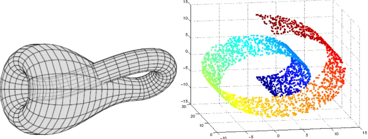
2.2.1.4 Manifold

As stated in section2.2.1.3, a given high-dimensional dataset may contain many fea-tures that are all from measurements taken, that are related to the same underlying cause. The manifold hypothesis [34,35] describes that the data generating distribution is assumed to concentrate near regions of low dimensionality.

In mathematics, a manifold is a topological space that resembles Euclidean space near each point [36], and can be perceived like a surface of any shape, in layman’s terms.

(33)

The use of the term manifold in machine learning is looser than its use in mathematics for practical reasons, where the data may not be strictly on the manifold, but only near it, the dimensionality may not be the same everywhere and the notion referred to in machine learning extends to discrete spaces [23]. The dataset lies along a low-dimensional man-ifold embedded in a high-dimensional space, where the low-dimensional space reflects the underlying parameters and high-dimensional space is the feature space.

(a) A klein bottle is an example of a manifold

[37].

(b) A manifold in a shape of a swiss-roll [38].

Figure 2.2: Manifold exemplified

2.2.2 Principal Component Analisys

Principal Component Analisys, or PCA, is a method of identifying patterns in data, excelling at data with high dimensionality where graphical representation is not an option. The goal of PCA is to extract the most important information, while compressing the size of the dataset and then analyze the structure of the observations reducing this way the possibility of overfitting [39].

First consider a X dataset that as mxn size where m represents the samples, a protein residue is a sample for example, and n represents the various features. PCA gives a choice on which type of matrix to use for analizying the data points, the covariance matrix and the correlation matrix. The covariance matrix retains the units of measurement, meaning that the different features must be comparable between themselves, it also makes changes to the scale, even by a similar constant, of the features, resulting in different results. The correlation matrix is dimensionless since it divides the value of covariance by the product of standard deviations which have the same units and the result is not influenced by a changing in the scale of the values. Since the features presented in section 2.1.2 do not have the same type of unit measurement, the use of correlation matrix may be more appropriate [40].

The core of PCA are the eigenvectors, or in this algorithm also called principal components, that represent the directions of the new feature space and the eigenvalues

(34)

that represent their magnitude explaining the variance of the data along the new feature axes. These are obtained by performing a eigendecomposition on the covariance matrix Σ, a matrix of size dxd with each element representing a covariance between two features. After having both eigenvalues and eigenvectors it is time to reduce the dimensionality of the original feature space. Since the eigenvectors have all a unit length of one, they can’t be used to predict which ones are better than others at conserving the most variance between the data points as possible, there is a need to analize the correspondent eigenvalues. This analysis consists in sorting the values in a descent manner by value and choose the top eigenvectors pretended. The number of eigenvectors to use depends for each context case and which level of variance is pretended to be saved. The most common way to find this number is just by calculating the explained variance from the eigenvalues that reveals how much variance can be related to each principal component.

Figure 2.3: Diagram showing three principal components. The order of the principal components follow the highest variance of the data [41].

PCA tries to find a linear subspace of lower dimensionality, such that the largest variance of the original data is kept. However, it has to be noted that the largest variance of the data does not necessarily represent the most discriminative information. Linear subspaces may not adequately represent the the underlying manifold on a dataset which may have some other nonlinear structure. Even when a linear projection on the data can find a representation with some number of dimensions, there is still a possibility of finding a more efficient representation that captures the data even better using a lower dimensional manifold. For this reason another algorithm is needed, one that finds a nonlinear subspace. It will be interesting to analyze what kind of lower dimension best represents the dataset.

(35)

2.2.3 Isomap

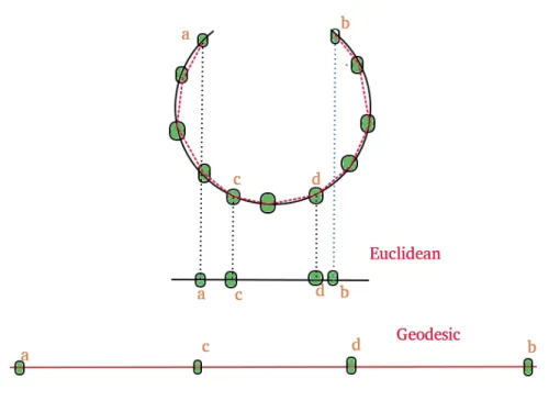
Isomap stands for isometric mapping and it is a nonlinear dimensionality reduction algorithm by trying to preserve the geodesic distances in a lower dimension. Due to euclidean distances being highly misleading in a nonlinear data structure, Isomap uses the geodesic distance, a distance that "follows"the manifold and because of that, holds off on the same data structure, giving a better estimation on the distance of two points [42]. This can be observed in figure2.4.

Figure 2.4: Differences between 1-D mappings of the two distance metrics. The mapping obtained with the euclidean distance gives off incorrect distances between the points while the geodesic distance gives a very accurate distance between the same points [43]

For this, first the algorithm must determine the neighbors of each point, either by a fixed radius or by using the k-nearest neighbors algorithm, or k-NN. In both situations one has to choose the lenght of the radius or the number of k neighbors. In k-NN a point is classified by a plurality vote of its neighbors, with the object being assigned to the class most common among its k-nearest neighbors. Then these neighborhood relation are used to construct a weighted graph. For the next step, an estimation of the geodesic distance between all pairs of points is needed while making sure that the resulting graph is fully connected. To calculate the shortest distance one can use the Djkstra’s algorithm, an algorithm that finds a shortest path tree from a single source node, by building a set of nodes that have minimum distance from the source. Finally one needs to compute a lower-dimensional embedding. This can be achieved by using the multilower-dimensional scaling

(36)

algorithm, or MDS, an algorithm that tries to find a set of vectors in p-dimensional space such that the matrix of euclidean distances among them corresponds as closely as possible to some function of the input matrix according to a criterion function called stress. The smaller the value returned by the stress function, the greater the correspondance between the two points. This algorithm can be perceived as a mathematical operation that converts a point-by-point matrix into a point-by-feature matrix.

Isomap gives the advantage of finding a nonlinear representation of the data, whereas PCA cannot. But this comes with extra concerns, namely, the sensitivy to noise where a few outlier points can break the mapping, the few free parameters that one can change making the algorithm rely mostly on the choice of the radius length, or k for the k-NN, and also the fact that Isomap usually performs poorly when the manifold is not well sam-pled and contains holes. For these reasons a final algorithm will be presented, which can function in a nonlinear subspace and do not have some of the requirements of Isomap.

2.2.4 Other Algorithms

In this subsections it will be presented algorithms that are fully implemented by python packages referred in section2.3.5.They will be used as comparison to the autoencoders that will be the main focus of this work.

2.2.4.1 t-Distributed Stochastic Neighbor Embedding

The aim of t-Distributed Stochastic Neighbor Embedding, or t-SNE, is to extract clus-tered local groups of samples, which can be beneficial to disentangle data that have many manifolds associated to them [44]. To achieve this t-SNE converts similarities between data points to joint probabilities, and with that, tries to minimize the Kullback-Leibler divergence between the joint probabilities of the higher-dimensional data and the lower-dimensional projected data. Since this divergence is not convex, diferent runs of the algorithm will return different results, but it is perfectly fine to run t-SNE several times, and select the solution with the lowest Kullback-Leibler divergence. This algorithm is computationally expensive, so passing first the data through a PCA algorithm can im-prove significatily that.

2.2.4.2 Multi Dimensional Scaling

The goal of Multi Dimensional Scaling, or MDS, is to place each data point in a lower-dimensional space such that the distances between the data points are preserved as well as possible in relation to the original space [45]. There are different variants of this

algorithm, including the metric multi dimensional scaling and the non-metric multi dimensional scaling. The first preserves the original distance metric, between points, as well as possible. That means that the distances in the higher-dimensional space are in the same metric as the ones of the lower-dimensional projected data. To the second

(37)

variant the important is not the metric of a distance value, but its value in relation to the distances between other pairs of data points. This means that if the distances between two different data points rank xth_{in the higher-dimensional space then they also have to} rank xthin the lower-dimensional projected data.

2.2.4.3 Local Tangent Space Alignment

The goal of Local Tangent Space Alignment, or LTSA, is based on the intuition that when a manifold is correctly unfolded, all of the tangent hyperplanes to the manifold will become aligned [46]. Like others algorithms described in this section first it will start by computing the neighborhood for each data point. Next it will calculate the local geometry of each neighborhood by its tangent space. Finally the algorithm will perform a global optimization to align all the local tangent spaces.

2.2.5 Auto Encoders

With the rise of processing power of computers neural networks became a recurrent topic in deep learning, since it offers advantages in pattern recognition that other unsu-pervised learning algorithms cannot, like the performance of the algorithm increase with the quantity of data available. An autoencoder is essentally a neural network that has the objective of copying is input to the output. The usefulness of an autoencoder relies on having a hidden layer that is smaller than the input layer, imposing the creation of a more compressed representation of the data. When the data has some latent representation structure, i.e. correlations between input features, it can be learned in the bottleneck of the autoencoder, also refered as code size, which is the smaller layer of an autoen-coder. There are two important operations in an autoencoder: the encoder, responsible for compressing the input into a latent-space representation and the decoder, responsi-ble for reconstructing the output from the latent-space representation. The decoder is symmetric to the encoder in terms of the layer structure [23].

With this the autoencoder can be represented as o = g(f (i)), where o tries to be as close as possible to i. That means that the algorithm will have to encapsulate the infor-mation from the input in h, saving in this representation the inforinfor-mation in a way that can be used to generate an output very close to the input. An autoencoder can be trained by minimizing the reconstruction error, L(o, i), which measures the differences between the input and the reconstruction. When constructing the model off an autoencoder one must balance the sensivity to the needs of the problem. The model must be sensitive enough in relation to the input so its reconstruction is accurate, but not so sensitive so the model does not simply copy the training data and be overfitting. This trade-off can be accomplished by using a loss function, a function that punishes the model when the output deviates from the input, combined with a regularizer, a parameter that tries to battle overfitting of the data. In real life problems, a scaling parameter can be added in front of the regularization term so that the trade-off can be more easily manipulated.

(38)

Figure 2.5: Example of an autoencoder with the diferent parts represented. The bottle-neck is formed where the encoder intersects the decoder, Y [47].

The most relevant properties of an autoencoder is the specificity of the data, where an autoecoder is only able to compress data similar to the training data, the lossiness of the output compared to the original inputs and the specialization of training instances that will perform better on specific types of input.

• Undercomplete Autoencoders: This type of autoencoders rely in a loss or penal-izing function that the algorithm tries to minimize. This minimization can be expressed by L(i, g(f (i))) where L penalizes g(f (i)) for being dissimilar in relation to i. This way the autoencoder can learn the most salient features. Since it does not have a regularization term, the model needs to have the number of nodes in the hidden layers restricted, so it won’t overfit the the training data.

• Sparse Autoencoders: This type of autoencoders can provide an information bot-tleneck without the need to reduce the number of nodes in the hidden layers. For this to happen it takes a training criterion with a sparsity penalty, Ω, on the code layer, h, in addition to the reconstruction error L(i, g(f (i))) + Ω(h), where g(h) is the decoder output and h the encoder output. This is useful when the objective is to learn features for other tasks like classification. This way the loss function penal-izes activations within a layer makes the model become more sensitive to specific attributes of the input data.

• Denoising Autoencoders: The idea behind this type of autoencoder is that the rep-resentation should be robust to the introduction of noise. For this the input must pass through a function that adds noise to it, that can be a random assignment of a subset of inputs to 0 with an arbitrary probability or can be also a gaussian noise that is a statistical noise having a probability density function equal to that of the normal distribution. Then the output is reconstructed from the corrupted input

(39)

and finally the loss function compares the output with the original input without noise.

Autoencoders are very flexible, in the sense that one can introduce nonlinear prob-lems by using a nonlinear activation function. This and the fact that the increase of features will result in a slower processing performance of PCA comparing with autoen-coders. Also the dataset does not have to fit into memory, and can be dynamically loaded up and trained with some variant of stochastic gradient descent, which is not the case for Isomap that forces the dataset to exist in memory. The main disadvantage of an au-toencoder is the fact that it is extremely uninterpretable, making nearly impossible to a human to visualize and understand the latent features. The different types of autoencoder have each different utilities based on their functioning. The undercomplete autoencoders have a smaller dimension for hidden layer compared to the input layer which helps to obtain important features from the data. The sparse autoencoders have the sparsity con-straint that prevents the output to be just a copy of the input, making the model less likely to overfit. The denoising autoencoders ensures that a a good representation can be robustly derived from corrupted or noisy input data and that helps with the task of re-covering a clean input that corresponds to the corrupted one. These differences between the functioning of the variations of the autoencoders will be empirically tested.

2.2.6 Last Considerations

The three chosen algorithms have all their advantages and disadvantages in relation to one another that are declared in the last chapters where the algorithms are described. It is important to refer that there is not one that is fully superior to other, making the dataset itself the chooser of the most appropriate algorithm.

Finally to assess the quality of the resulting low-dimensional data representations, one can measure the performance of the algorithms withtrustworthiness and continuity to evaluate to what extent the local structure of the data is retained [48]. The trustwhortiness measures the proportion of points that are close togheter in the low-dimensional space:

T (k) = 1 − 2 nk(2n − 3k − 1) n X i=1 X j∈U_i(k) (r(i, j) − k),

where r(i, j) is the the rank of the low-dimensional datapoint j according to the pair-wise distances between the low-dimensional datapoints. The variable U_i(k)indicates the set of points that are among the k nearest neighbors in the low-dimensional space but not in the high-dimensional space.

The continuity is measured by:

C(k) = 1 − 2 nk(2n − 3k − 1) n X i=1 X j∈V_i(k) ( ˆr(i, j) − k),

(40)

where ˆr(i, j) is the rank of the high-dimensional datapoint j according to the pairwise distances between the high-dimensional datapoints and V_i(k) is the set of points that are among the k nearest neighbors in the high-dimensional space but not in the low-dimensional space.

Besides these techniques to compare the performance of the different reductions there is a need to use classification algorithms used to classify the contacts between the molecules. One of the algorithms is a Naive Bayes Classifier with the addition of a constraint-based method for improving protein docking results, used in another work [49], that utilizes combinations of features for improving protein docking. Another work worth to be cited is HawkRank [50], a scoring function used in the sampling stage of protein–protein docking using energy terms, including van der Waals potentials, electro-static potentials and desolvation potentials. This function uses weighted potentials from different features and sums everything to the final score. It is also worth mentioning the dataset used for the benchmarking, the ZDOCK benchmark collection, more specifically the fourth version [51]. This benchmark is a collection of distinct protein docking test cases that was used for evaluating HawkRank to other algorithms. These two algorithms are examples of how to test the uselfuness of the extracted features. There are other examples that can be chosen, using a criterion of how simple is to adapt the models to the extracted features.

2.3 Tools

In this section it will be presented the software technology that exists that can be used to build the machine learning algorithms to solve the problem that is presented in this thesis. Since the programming language chosen is Python, due to the sheer amount of packages related to machine learning and also parsing and plotting data, the frameworks considered must allow to work with Python.

2.3.1 Theano

Theano [52]is a Python library that is used to define, optimize, and evaluate mathemat-ical expressions, especially the ones with tensors. Using Theano, it is possible to surpass the language C on a CPU by many orders of magnitude by taking advantage of recent GPUs. The combination of computer algebra system (CAS) with optimizing compila-tion is particularly useful for tasks in which very complex mathematical expressions are evaluated repeatedly and evaluation speed is of most importance. For situations where many different expressions are each evaluated once, Theano can minimize the amount of compilation/analysis overhead, but still provide symbolic features such as automatic differentiation. The Theano project stopped having new relases after version 1.0.0 in 2017, which can be a deciding factor in the selection of a framework.

(41)

2 . 3 . T O O L S

2.3.2 Tensorflow

TensorFlow [53] was originally developed by researchers on the Google Brain team within Google’s Machine Intelligence Research organization for the purposes of conduct-ing machine learnconduct-ing and deep neural networks research. A computational framework, with a stable Python and C API, for building machine learning models using data flow graphs. The nodes of the graph are mathematical operations, whereas the edges repre-sent tensors that flow between them. One of the key functionalities of Tensorflow is it’s flexible architecture enables deployment computation to one or more CPUs or GPUs in a desktop, server, or mobile device without rewriting code. It can be used to lower-level APIs to build models by defining a series of mathematical operations or can be used for higher-level APIs to specify predefined architectures, such as linear regressors or neural networks. These reasons make Tensorflow a good framework to use in this work.

2.3.3 PyTorch

PyTorch [54] is an open source machine learning framework for python developed by Facebook research group. It allows one to flexible experiment and produce in an efficient manner through a hybrid front-end, distributed training and a vast amount of tools and libraries. It takes advantage of native support for asynchronous execution of collective operations and peer-to-peer communication. These reasons makes PyTorch, as it happened with Tensorflow, to be considered to be used in this work. This framework will probably be used if the work cannot run on top of Tensorflow, making this framework asafety net.

2.3.4 Keras

Keras [55] is more of an interface rather than a standalone machine-learning framework that was developed with the objective of enabling faster experimentation. It offers a high-level set of abstractions that make it easy to develop deep learning models on top of Tensorflow or Theano. For these reasons this framework will be tested on top of Tensorflow.

2.3.5 Python Libraries

These are language dependent libraries that are going to be used, many of them widely used in the machine learning context.

• Scikit-Learn: a Python free to use library with a large number of state-of-the-art machine learning algorithms for supervised and unsupervised problems[56]. • SciPy: a free and open-source library built for Python that contains a wide array of

tools for optimization, linear algebra, integration, interpolation, special functions, signal and image processingand other tasks common in science and engineering[57].

(42)

• Matplotlib: a free and open-source plotting Python library which produces a very wide variety of graphs and plots namely like histograms, bar charts, power spectras, error charts between others[58].

• Pandas: Pandas, or Python Data Analysis Library, is a free Python library under the BSD license that is useful for data manipulation and analysis. One of the main features of this library is the existence of DataFrame objects that make the data manipulation more accessible to deal with [59].

• OpenBabel: a open Python library under the GNU GPL license where the main fo-cus is to search, convert, analyze, or store data from molecular modeling, chemistry, solid-state materials, biochemistry and other related areas. OpenBabel version 2.3 interconverts over 110 formats[60].

• BioPython: a Python library under the bioinformatics license that allows the cre-ation of reusable modules and classes and includes parsers for various file formats, access to online services, interfaces to a big number of programs between other features [61].

• PyMOL a Python library for visualization of molecular complexes free of use and distributed with a Python license[62].

(43)

C

h

a

p

t

e

r

3

E x p e r i m e n ta l Wo r k

This chapter is composed by the details about the implementation of the whole system used in this thesis including the preprocessing of the data algorithms and presentation of results.

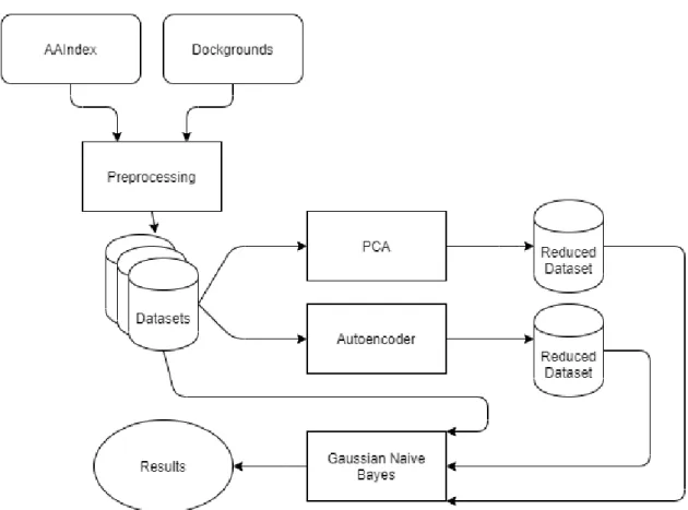
3.1 Implementation

The implementation of the system consists of the following parts:

• Preprocessing: Starting with.pdb files downloaded from Dockground and features downloaded from the AAIndex, this part will transform to.csv files which consist of the data points of the contacts and the neighbours with the corresponding features and labels that will be used by the algorithms.

• Algorithms: The algorithms used are an implemented Autoencoder and a PCA for dimensionality reduction and a Naive Bayes classifier to evaluate how much of a improvement the reduced features will be.

• Presentation: Finally the graphic representation of the results are also implemented to a more easy human interpretation.

In figure3.1it is represented a diagram with the principal components of the imple-mentation.

3.2 Data

This section will discuss the treatment of the data since its origin to the moment that will be used by the algorithms implemented.

(44)

C H A P T E R 3 . E X P E R I M E N TA L WO R K

Figure 3.1: Diagram of the principal pipeline of the project

3.2.1 Data Source, Features and Labels

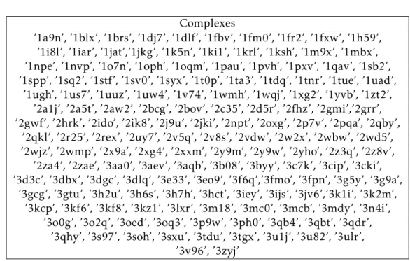
The proteins files are downloaded from theDockground website [21], where each pro-tein file consists of a set composed by two parts: the first part is a.pdb file with the first part of the complex and the second part includes a one near native and ninety nine in-correct docking poses for the specific protein-protein complex in which the first model is the correct one. The starting total of complexes is 164 but after eliminating files which originated problems with the parsing the final number of complexes processed decreases to 156. Table3.1shows the complete set of complexes that are used in this dissertation.

The files names represent the code id of the complex with four alphanumeric char-acters. The code of the complex is the same for both the receptor and the ligand, with the only difference being the chain for each one. The receptor has one chain and the other ligand models are all represented by a different chain from the receptor but equal between them.

The features used are extracted from theAAIndex database, in which two parts of the database are used, the first and the third that are composed of the amino acid index of 20 numerical values and the statistical protein contact potentials, respectively. In total there are 566 features from the first part and 33 features from the third part, which were analyzed to choose the ones that are relevant.

(45)

3 . 2 . DATA

Complexes

’1a9n’, ’1blx’, ’1brs’, ’1dj7’, ’1dlf’, ’1fbv’, ’1fm0’, ’1fr2’, ’1fxw’, ’1h59’, ’1i8l’, ’1iar’, ’1jat’,’1jkg’, ’1k5n’, ’1ki1’, ’1krl’, ’1ksh’, ’1m9x’, ’1mbx’, ’1npe’, ’1nvp’, ’1o7n’, ’1oph’, ’1oqm’, ’1pau’, ’1pvh’, ’1pxv’, ’1qav’, ’1sb2’, ’1spp’, ’1sq2’, ’1stf’, ’1sv0’, ’1syx’, ’1t0p’, ’1ta3’, ’1tdq’, ’1tnr’, ’1tue’, ’1uad’,

’1ugh’, ’1us7’, ’1uuz’, ’1uw4’, ’1v74’, ’1wmh’, ’1wqj’, ’1xg2’, ’1yvb’, ’1zt2’, ’2a1j’, ’2a5t’, ’2aw2’, ’2bcg’, ’2bov’, ’2c35’, ’2d5r’, ’2fhz’, ’2gmi’,’2grr’, ’2gwf’, ’2hrk’, ’2ido’, ’2ik8’, ’2j9u’, ’2jki’, ’2npt’, ’2oxg’, ’2p7v’, ’2pqa’, ’2qby’,

’2qkl’, ’2r25’, ’2rex’, ’2uy7’, ’2v5q’, ’2v8s’, ’2vdw’, ’2w2x’, ’2wbw’, ’2wd5’, ’2wjz’, ’2wmp’, ’2x9a’, ’2xg4’, ’2xxm’, ’2y9m’, ’2y9w’, ’2yho’, ’2z3q’, ’2z8v’,

’2za4’, ’2zae’, ’3aa0’, ’3aev’, ’3aqb’, ’3b08’, ’3byy’, ’3c7k’, ’3cip’, ’3cki’, ’3d3c’, ’3dbx’, ’3dgc’, ’3dlq’, ’3e33’, ’3eo9’, ’3f6q’,’3fmo’, ’3fpn’, ’3g5y’, ’3g9a’,

’3gcg’, ’3gtu’, ’3h2u’, ’3h6s’, ’3h7h’, ’3hct’, ’3iey’, ’3ijs’, ’3jv6’,’3k1i’, ’3k2m’, ’3kcp’, ’3kf6’, ’3kf8’, ’3kz1’, ’3lxr’, ’3m18’, ’3mc0’, ’3mcb’, ’3mdy’, ’3n4i’,

’3o0g’, ’3o2q’, ’3oed’, ’3oq3’, ’3p9w’, ’3ph0’, ’3qb4’, ’3qbt’, ’3qdr’, ’3qhy’, ’3s97’, ’3soh’, ’3sxu’, ’3tdu’, ’3tgx’, ’3u1j’, ’3u82’, ’3ulr’,

’3v96’, ’3zyj’

Table 3.1: The complexes used in this dissertation extracted fromDockground

3.2.2 Data Preprocessing

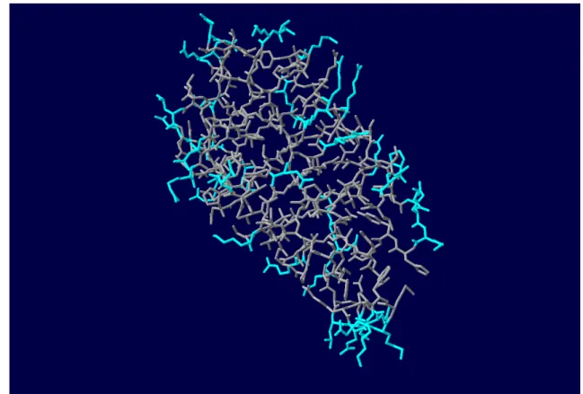
Since the data necessary to be used in the algorithms originates from various sources there is a need to collect and preprocess all of the information necessary to the creation of the dataset. As stated in [16], almost all contacts are made by the residues in the complex that are in the surface. Using theBioPython library, the residues that are present in the surface can be collected by their ASA value and stored for the next steps. The value of ASA used as a threshold to define if a residue is in the surface or interior for the purpose of this dissertation is 30%.

The next step is to find the residues on the surface of both complexes that are close to each other. In [63] it is mentioned that the contacts between residues can be at maximum 8 angstroms. There are going to be tested distances of 2, 4, 6 and 8 to better compare how the distance influences the classifier predictions. The residues neighbours considered are also only in the surface of the complex and as what happens with the distance of contacts. A range of values between 2 and 6 angstroms are used and there are several different distances used to define the neighbourhood of residues of the residue in contact.

Now that the contacts and their respective neighbourhoods are selected, the next step is to find the corresponding features for each of them. The first features that are used are the ones from AAindex3 and each feature has a corresponding value for each type of contact. There are 33 features that were added to each contact. The second type of features are the ones fromAAindex1 and these have a value associated with each residue. There are 566 existing features, but since many of them are only valid for certain cases, likeHelix termination parameter at position j-2,j-1,j and repetitions in the indices as result

(46)

C H A P T E R 3 . E X P E R I M E N TA L WO R K

Figure 3.2: Representation of the surface residues of a protein. The light blue residues represent the surface. This image was taken from the A chain from protein 1a9n with the help of the Swiss PDB Viewer.

of different experiments, the number of features utilizes will have to be trim down. After this step the number of features are 97 and each of them are used twice for each contact since each contact is represented by two residues resulting in 194 features for each contact. Additionally the minimum, maximum and mean values of each of theAAindex1 are used in each neighbourhood of each of the contacts residues performing more 582 features. The last type of features are performed by an algorithm developed that simply returns the number of different types of residues for each complex and each neighbourhood of the contacts. Considering that there are twenty types of amino acids, at least for the purpose of this dissertation, each contact will have eighty additional features for each contact, 20 for each contact residue and 20 to each contact residue neighbourhood. In the end each contact will have a total of 695 distinct features.

For each contact it is added a label designating the name of the protein at which the contact belong. These are useful in the next steps for analyzing the data. These steps result in a.csv file with each row representing a contact and the columns representing the features extracted in the previous steps. The labels that serve to distinguish the true contacts from the false will be simply the value of 1 to the true contacts and 0 for the false ones.