UNIVERSIDADE DE ÉVORA
ESCOLA DE CIÊNCIAS E TECNOLOGIAS
DEPARTAMENTO DE BIOLOGIA
“Identificação de fatores determinantes que
influenciam o atropelamento de serpentes no
sul de Portugal”
Eliana Denise Simões Loureiro
Orientação: Paulo Alexandre Cunha e Sá de Sousa
Mestrado em Biologia da Conservação
Dissertação
ii
Mestrado em Biologia da Conservação
Dissertação
“Identificação de fatores determinantes que influenciam o
atropelamento de serpentes no sul de Portugal”
Eliana Denise Simões Loureiro
Orientador
Paulo Alexandre Cunha e Sá de Sousa
iii
Master of Conservation Biology
Thesis
“Identifying key factors that influence snake roadkill in
southern Portugal”
Eliana Denise Simões Loureiro
Supervisor
Paulo Alexandre Cunha e Sá de Sousa
iv
If you’re not prepared to be wrong, you’ll never
come up with anything original.
v
A
GRADECIMENTOS
Agradeço ao Ricardo Leite porque tudo é mais fácil quando se tem um companheiro ao lado, ainda mais por me ter aturado todos os dias em que estive agarrada à tese.
Agradeço a família do Ricardo pela paciência e compreensão que demonstraram todos os dias.
Agradeço à Inês Alves por me fornecer o espaço que permitiu inspirar -me nos momentos mais nheca que as teses conseguem sempre tão bem demonstrar e à Inês Balula por não deixar que a vida social de certas e determinadas toupeiras morra nas mãos da tese.
Agradeço ao António Matos por me ter prontamente ajudado a rever a tese, mesmo tão em cima da hora.
Agradeço igualmente a todos os restantes amigos que de uma forma ou de outra compartilharam muitos momentos ao longo desta caminhada tão importante.
Agradeço ao meu orientador Paulo Sá -Sousa e ao António Mira pelas imprescindíveis sugestões que influenciaram grandemente a direcção que tomei nesta tese.
Agradeço também ao António Mira e ao projecto “Move” por fornecer os dados de atropelamento que tornam possível a realização desta tese.
Agradeço principalmente à minha família por fazerem de mim o que sou hoje. À minha mãe por fazer -me mostrar que é possível erguer -me nos momentos mais difíceis, ao meu irmão por aturar esta mana mais velha (depois disto vai ser pior, vais ver), às minhas avós sempre preocupadas com o meu bem -estar e aos meus avôs e tio por me fazerem ver o outro lado das coisas.
vi
RESUMO
“Identificação
de fatores
determinantes
que
influenciam
o
atropelamento de serpentes no sul de Portugal”
O impacto das rodovias é bastante marcado ao nível da fauna vertebrada terrestre, sendo comum encontrar serpentes atropeladas. Com base num registo diário de 2 anos analisaram-se padrões espaciais no atropelamento de serpentes em quatro troços de estradas ao longo de 50.6 km. Os dados de atropelamento foram analisados ao nível da comunidade de serpentes e das espécies principais. O maior atropelamento da comunidade de serpentes e de Rhinechis scalaris ficou assim associado a maior cobertura de Montado, enquanto a cobertura arbustiva foi então associada a uma menor probabilidade de atropelamentos. A rugosidade do terreno e os terrenos agrícolas revelaram-se também importantes no padrão de atropelamento até valores intermédios. Hemorrhois hippocrepis estava fortemente ligada às áreas influenciadas pelas atividades humanas, enquanto que Natrix maura atropeladas foram associadas à proximidade de charcos. Além disso, evidenciou-se um maior risco de atropelamento em estradas nacionais do que em estradas municipais. Assim, demonstrou-se a importância de considerar elementos paisagísticos para melhor compreender o atropelamento de serpentes.
Palavras -chave: Colubridae, serpentes, padrão espacial de atropelamento, Inferência multimodelo, Alentejo
vii
ABSTRACT
“Identifying key factors that impact snake roadkill in southern Portugal”
The impact of roads is a serious issue among terrestrial vertebrate fauna, in fact snakes are frequently found dead on roads. To analyse snake roadkill spatial patterns, roadkill data was collected over a 2 year period from 4 road stretches that are 50.6 km long. The data was analysed at the snake community and species level. Snake community and Rhinechis scalaris roadkill were associated to Montado cover, while shrub cover lowered the chance of roadkill. Terrain roughness and agricultural land were also an important roadkill feature occurring up to intermediate levels. Increased
Hemorrhois hippocrepis roadkill was highly associated to human influenced areas,
while Natrix maura roadkill was strongly linked to the proximity of water sources. The risk of snake roadkill was higher in national roads than in municipal roads. In brief, taking into account landscape factors seems to be an important step to improve our understanding on snake roadkill.
Keywords: Colubridae, serpents, roadkill spatial pattern, multimodel inference, Alentejo
viii
TABLE OF CONTENTS
RESUMO vi ABSTRACT vii LIST OF FIGURES x LIST OF TABLES xi FORWARD 1 INTRODUCTION 1Impacts of roads on fauna 1
Factors influencing snake roadkill 2
Objectives 4
MATERIAL & METHODS 4
Study Area 4
Snakes in Portugal 6
Roadkill Surveys 6
Statistical Analysis 8
Response and Explanatory Variables 10
Model Development and Selection 11
Multimodel Inference 16
ix
DISCUSSION 25
CONCLUDING REMARKS 30
REFERENCES 32
APPENDIX 41
APPENDIX A – ENVIRONMENTAL VARIABLES RESPONSE CURVES FOR SNAKE
COMMUNITY AND INDIVIDUAL SPECIES RESPONSE VARIABLES. 42
APPENDIX B – MODELS, RANKING AND CALCULATIONS OF MODELS GENERATED
x
LIST OF FIGURES
FIGURE 1–LANDSCAPE SURROUNDING SURVEYED ROADS (ADAPTED FROM “MOVE” PROJECT). 5
FIGURE 2–PHOTOGRAPHS OF THE SNAKE SPECIES FOUND IN SOUTHERN PORTUGAL. 7
FIGURE 3-STUDY AREA WITH A 1000m BUFFER DISTANCE AROUND THE SURVEYED ROADS (ADAPTED FROM “MOVE” PROJECT) AND SNAKE ROADKILL NUMBER. 8
FIGURE 4–SNAKE COMMUNITY RELATIONSHIPS BETWEEN ROADKILL OCURRENCE AND a) ROUGHNESS
INDEX OR b)AGRICULTURAL LAND. 20 FIGURE 5 – H. hippocrepis RELATIONSHIPS BETWEEN ROADKILL OCURRENCE AND a) HUMAN
INFLUENCED AREA OR b)DISTANCE TO RIPARIAN GALLERY. 21
FIGURE 6–R.scalaris RELATIONSHIPS BETWEEN ROADKILL OCURRENCE AND a)ROUGHNESS INDEX OR
b)AGRICULTURAL LAND. 22
FIGURE 7–N.maura RELATIONSHIPS BETWEEN ROADKILL OCURRENCE AND a)WATER SOURCE OR b)
OPEN AREA. 23
FIGURE 8 – M. monspessulanus RELATIONSHIP BETWEEN ROADKILL OCURRENCE AND ROUGHNESS
xi
LIST OF TABLES
TABLE 1–SEVERAL SNAKE FEATURES THAT MAY INFLUENCE ROADKILL IN SOUTHERN PORTUGAL. 9 TABLE 2- SEQUENTIAL MAIN STEPS APPLIED IN MODEL DEVELOPMENT, SELECTION AND MULTIMODEL INFERENCE WHETHER FOR THE FOUR INDIVIDUAL SPECIES (R. scalaris, M. monspessulanus, N. maura,H.hippocrepis) OR FOR THE SNAKE COMMUNITY RESPONSE VARIABLES. 14
TABLE 3-DESCRIPTION OF THE EXPLANATORY VARIABLES USED IN MODEL SELECTION AND MULTIMODEL
INFERENCE. 17
TABLE 4–SNAKE ROADKILL COUNT FOR FOUR ROADS SURVEYED IN THE STUDY AREA FROM 16 OF MARCH
2010 TO 15 OF MARCH 2012. 18
TABLE 5-MORAN’S I,Z AND P VALUES FOR THE SNAKE COMMUNITY AND INDIVIDUAL SPECIES1. 18
TABLE 6-BUFFER SIZE FOR THE SNAKE COMMUNITY AND INDIVIDUAL SPECIES. 19
TABLE 7 - FINAL GLOBAL MODELS FOR THE SNAKE COMMUNITY AND RESPONSE VARIABLES OF FOUR
SPECIES. 19
TABLE 8 - MODEL AVERAGING AND VARIABLE RELATIVE IMPORTANCE (VRI) RESULTS FOR THE SNAKE
COMMUNITY. 20
TABLE 9- MODEL AVERAGING AND VARIABLE RELATIVE IMPORTANCE RESULTS FOR THE HORSE WHIP SNAKE Hemorrhois hippocrepis. 21 TABLE 10-MODEL AVERAGING AND VARIABLE RELATIVE IMPORTANCE RESULTS FOR THE LADDER SNAKE
Rhinechis scalaris. 22
TABLE 11-MODEL AVERAGING AND VARIABLE RELATIVE IMPORTANCE RESULTS FOR THE VIPERINE SNAKE
Natrix maura. 23
TABLE 12 - MODEL AVERAGING AND VARIABLE RELATIVE IMPORTANCE RESULTS FOR THE RAT SNAKE
Malpolon monspessulanus. 24
TABLE A1-AKAIKE WEIGHTS (WI) OF UNIVARIATE MODELS USED TO EXPLORE ALTERNATIVE RESPONSE
CURVES IN SNAKE COMMUNITY AND INDIVIDUAL SPECIES (ENVIRONMENTAL VARIABLES OF EACH BUFFER AND LANDSCAPE METRICS WITHOUT BUFFER LIMIT). 42
xii
TABLE B1-MODELS SELECTED FOR THE SNAKE COMMUNITY WITH A ∆AICC<6 AND EXPLAINED DEVIANCE
(D2),AICC AND ∆AICC VALUES. 44
TABLE B2 - MODELS SELECTED FOR THE HORSE WHIP SNAKE Hemorrhois hippocrepis WITH A
∆AICC<6 AND EXPLAINED DEVIANCE (D2),AICC AND ∆AICC VALUES. 47
TABLE B3-MODELS SELECTED FOR THE LADDER SNAKE Rhinechis scalaris WITH A ∆AICC<6 AND
EXPLAINED DEVIANCE (D2),AICC AND ∆AICC VALUES. 49
TABLE B4 - MODELS SELECTED FOR THE VIPERINE SNAKE Natrix maura WITH A ∆AICC<6 AND EXPLAINED DEVIANCE (D2),AICC AND ∆AICC VALUES. 50
TABLE B5-MODELS SELECTED FOR THE RAT SNAKE Malpolon monspessulanus WITH A ∆AICC<6 AND EXPLAINED DEVIANCE (D2),AICC AND ∆AICC VALUES. 52
1
FORWARD
This dissertation text is mostly set as a scientific paper in order to facilitate its final publication as soon as possible after the public defence of this thesis. Despite leaving some paragraphs in the text as explanatory views, I found it important for a better judgment in terms of the dissertation. However, the final text and figures aiming the future article may be a bit more succinct for editorial reasons. Nevertheless, I am the main author of the following text for all purposes.
INTRODUCTION
Impacts of Roads on Fauna
Roads are an important physical structure that provide connections between populated areas and are often considered an essential infrastructure to improve the development and productivity of a region (Coffin 2007). However, with the increased development of road networks in the last century, environmental impacts on fauna have been a growing issue in recent years (Bekker 2003; Coffin 2007).
The impacts of roads on fauna start with the construction phase and continue to disrupt the natural environment with its daily use. Besides road location determining the magnitude to which wildlife will be exposed, it also influences surroundings up to 100 -800 m beyond the road’s edges (Andrews, Gibbons & Jochimsen 2006; 2008). As a result, direct impacts usually consist of wildlife vehicle collisions, while indirect impacts range from habitat loss, habitat fragmentation and degradation to behavioural change of wildlife (Brito & Álvares 2004; Spellerberg 1998; Underhill & Arnold 2000).
Furthermore, animals may avoid roads, in which case a barrier effect is created (Andrews, Gibbons & Jochimsen 2006; van Langevelde, Dooremelan & Jaarsma 2009). If a road creates an impermeable barrier to animal movement then demography, population structure and genetic diversity may be modified (Brito & Álvares 2004). Even if roads do not pose a barrier, populations may still be at risk if a significant proportion is killed by roads and not compensated by higher birth rates (Gomes et al. 2009).
2 Factors Influencing Snake Roadkill
The extent to which roads impact snake populations is still poorly understood. One of the main reasons for this omission is due to the cryptic nature of these species, along with the failure to have a standard fauna sampling method that can adequately detect them (Dorcas & Willson 2009; Mcdonald 2012). Despite the sampling issues, it is clear that roadkill is affecting several snake species (Colino-Rabanal & Lizana 2012). In North America, roadkill studies have already demonstrated considerable damage to snake populations (Jochimsen 2006; Rosen & Lowe 1994). Also, a long term study about population viability on a snake species concluded that road mortality of more than 3 adult females per year was enough to increase the extinction probability to >90% (Row, Blouin -Demers & Weatherhead 2007). Lastly, results from another study suggested that populations of large snake species are reduced by 50% or more up to a distance of 450 m from roads with moderate use (Rudolph et al. 1999).
Understanding the impacts of roadkill in snake populations is essential for their conservation, as snakes play an important ecological role both as predators and prey in different ecosystems (Pragatheesh & Rajvanshi 2013). Snakes have several ecological traits that increase their probability of suffering a vehicle collision mentioned in the literature (Colino-Rabanal & Lizana 2012). Since snakes have a long life span and mature slowly, they usually present a low reproductive rate and show a natural low adult mortality. These traits add up to a number of characteristics that make snake mortality in roads an increased risk for populations (Hartmann, Hartmann & Martins 2011) and altogether make population dynamics extremely vulnerable to adult mortality (MacKinnon, Moore & Brooks 2005). The snake’s ability to cross a road can also be influenced by speed and defensive behaviours which are features that greatly vary from species to species. Also, matters can be aggravated when human and animal activities overlap as some snakes show a crepuscular behaviour during parts of the year that may match with rush -hour traffics (Andrews, Gibbons & Jochimsen 2006). Furthermore, although some snakes flee from danger as an initial response, others immobilize themselves hindering their chance to cross the road safely (Andrews, Gibbons & Jochimsen 2006). Nevertheless, research has shown that snakes tend to cross roads perpendicularly taking the shortest possible route (Andrews & Gibbons 2005; Shine et al.
3
2004), thus probably bettering their chances to cross successfully. In addition, snakes may use roads for their thermoregulation needs, favouring paved roads for its suitable heating surface (e.g. tigmotactism) and therefore increasing their vulnerability to roadkill (Andrews, Gibbons & Jochimsen 2006; Brito & Álvares 2004). This behaviour is particularly noticeable in the ladder snake that often takes advantage of the warm surface roads provide at night (Pleguezuelos 2009b). Also an important element for snake roadkill to occur is snakes’ movement patterns. These patterns are mainly driven by snakes’ breeding or migration periods or can simply refer to attending their basic needs (e.g. prey searching) and highlight the dispersive nature and temporal trends of snake species (Bonnet, Naulleau & Shine 1999; Brito & Álvares 2004; Jochimsen 2006). For example, the male Montpellier snake is more likely to be found dead on roads in the mating season due to their greater mobility in this season (Pleguezuelos 2009a). In autumn, juveniles after birth also have a higher probability of being run over when they start dispersing (Pleguezuelos 2009a).
Reports about snake mortality in roads go far back as the fifties (e.g. Campbell 1953; Hellman & Tellford 1956). However, investigation on why roadkill occurs has only started in recent years (Colino-Rabanal & Lizana 2012). Even with an increasing number of published articles arising, only a few are related to snake mortality in roads. Indeed, most published papers on the subject are from North American studies (Andrews & Gibbons 2005; Clark et al. 2010; Enge & Wood 2002; Gibson & Merkle 2004; Jochimsen 2006; Roe, Gibson & Kingsbury 2006; Row, Blouin -Demers & Weatherhead 2007; Rudolph et al. 1999; Shine et al. 2004), with only a few papers being published elsewhere (Bonnet, Naulleau & Shine 1999; Ciesiołkiewicz, Orłowski & Elżanowski 2006; Hartmann, Hartmann & Martins 2011; Pragatheesh & Rajvanshi 2013). In Portugal, one paper has been published by Brito & Álvares 2004 identifying viper roadkill patterns (age, sex and seasonal activity).
These studies have generally investigated temporal patterns and snake behaviours in roads, while only a few investigated the influence of spatial patterns (Enge & Wood 2002; MacKinnon, Moore & Brooks 2005; Pragatheesh & Rajvanshi 2013). Spatial patterns regarding habitat characteristics influencing wildlife movement may have an important
4
role in identifying major roadkill spots (Clevenger, Chruszcz & Gunson 2003; Forman & Alexander 1998).
Investigating the spatial patterns of snakes should give an important contribution towards understanding the role of spatial features in snake road mortality. After all, snakes in Portugal are no exception to the impact of roads as roadkill is one of the major threats for this group (Loureiro et al. 2010). In Portugal, more than 30% of recently registered specimens of R. scalaris were found dead on roads (Pleguezuelos 2009b).
Objectives
Since one knows that snakes are being killed in roads and that they play an important role in the ecosystem, it is essential to understand roads impacts in snake populations. Thus, the main objective of this study is to understand the influence of spatial factors in snake roadkill and therefore to determine the patterns and importance of environmental factors. The specific objectives are: to describe the ecology and biology of snakes in the study area linked to roadkill; identify the spatial factors that could be influencing roadkill in snakes; describe the spatial patterns of factors influencing roadkill.
Looking ahead, the results of this study should help recognize landscape’s key factors linked to snake roadkill and may be used in future studies, improving road management practices or mitigation planning.
M
ATERIAL
&
M
ETHODS
Study AreaThis study was conducted in the southern part of Portugal, in the Alentejo Central region (NUT III), comprising the municipalities of Évora and Montemor -o -Novo. The study area includes consecutive stretches of four roads along 50.6 km that, altogether, draw an irregular square: two national roads (N114 and N4) and two municipal roads (M370 and M529) – see Figure 1. Also, the highway (A6) is located nearby the N114 road.
5
FIGURE 2–LANDSCAPE SURROUNDING SURVEYED ROADS (ADAPTED FROM “MOVE” PROJECT).
Alentejo Central’s main landscape has been the so -called “Montado”. It consists mainly of an agrosilvopastoral ecosystem, mostly composed by cork (Quercus suber) or holm oak trees (Q. rotundifolia), shaping as a savanna like land cover pattern that is known for its cork production, as well as for its multiple supplementary productions that supports a diversity of ecosystems and biodiversity (Correia, Ribeiro & Sá -Sousa 2011; Godinho, Santos & Sá -Sousa 2011).
Being a type of Mediterranean region, the Alentejo Central’s climate has broad thermal ranges and quite different seasons with the hot dry season averaging 20 to 23 ºC and low rainfall (June to October) and the cool wet season averaging 10 to 15ºC with rainfall superior to 80mm (Galantinho & Mira 2008).
6 Snakes in Portugal
According to Carrascal & Salvador (2009) and the updated IUCN (2013), there are ten species of snakes distributed in Portugal: two vipers (Viperidae), two Natricidae, one Psammophiidae and five Colubridae. Among them, a total of seven species occur in southern Portugal (Table 1; Figure 2). These are mostly distributed through Western Europe and North Africa, generally occupying Mediterranean environments.
Table 1 summarizes some snake features (taken elsewhere from Carrascal & Salvador 2009 and Loureiro et al. 2010) that may influence road crossing. Different characteristics may have rather different impacts in the snake’s vulnerability to roadkill. For example, in the Iberian Peninsula some snake species have an active foraging behaviour during the day period that may make them more vulnerable to roadkill (Malkmus 2004; Pleguezuelos 2009; Salvador & Pleguezuelos 2002).
Roadkill Surveys
The road circuit (Figure 1) was surveyed daily from 16 of March 2010 to 15 March 2012, often in the morning. These roads differ in their features, mainly in their traffic flow. In brief, the national roads have a medium/high traffic (<10000 vehicles/day), while more local roads have a low traffic (<4000 vehicles/day, EP 2005). Snake roadkill was surveyed by car at a low speed (15 - 20km/h) in both road directions.
A global positioning system (GPS) was used to set the geographic coordinates of each snake carcass found on the pavement. Species name, age and sex were also recorded on the spot whenever possible. Finally, carcasses were removed from the road, avoiding double counting. Figure 3 shows the number of recorded snakes killed in roads during the course of the survey.
7
FIGURE 2–PHOTOGRAPHS OF THE SNAKE SPECIES FOUND IN SOUTHERN PORTUGAL.
© ©©AAA...SSSaaalllvvvaaadddooorrr... Natrix maura Hemorrhois hippocrepis © ©©JJJ...MMM...PPPllleeeggguuueeezzzuuueeelllooosss... Malpolon monspessulanus Coronella girondica
Macroprodonton brevis Rhinechis scalaris
© ©©JJJ...MMM...PPPllleeeggguuueeezzzuuueeelllooosss... © ©©JJJ...MMM...PPPllleeeggguuueeezzzuuueeelllooosss... ©©©AAA...SSSaaalllvvvaaadddooorrr... Natrix natrix © ©©IIIñññiiigggoooMMMaaarrrtttííínnneeezzz---SSSooolllaaannnooo... . © ©©PPPeeedddrrroooGGGaaalllááánnn...
8
FIGURE 3 -STUDY AREA WITH A 1000m BUFFER DISTANCE AROUND THE SURVEYED ROADS (ADAPTED
FROM “MOVE” PROJECT) AND SNAKE ROADKILL NUMBER.
Statistical Analysis
To investigate the importance of spatial factors and find patterns and magnitudes of parameters influencing roadkill, Generalized Linear Models (GLM) were built using a Poisson error distribution with a log link function. Models developed were used for model selection and multimodel inference (MMI) within an information theoretic approach.
9
TABLE 1– SEVERAL SNAKE FEATURES THAT MAY INFLUENCE ROADKILL IN SOUTHERN PORTUGAL.
a -IUCN Red List of Threatened Species (IUCN 2013); b -Enciclopedia virtual de los vertebrados españoles (Carrascal & Salvador 2009); c-Exception in southwest Iberian Peninsula, it is generally nocturnal; dAtlas dos Anfíbios e Répteis de Portugal (Loureiro et
al. 2010); e mean snout -vent length (SVL), except for C. girondica and N. natrix.
Scientific Name a English a & Portuguese d
Main Prey b Biotope b (study area) Abundance a Size b SVL e (mm) Foraging Mode b Activity b Home Range b (ha) Seasonal Activity b Colubridae Coronella girondica Southern Smooth Snake Cobra lisa bordalesa Lizards Arthropods Grassland Open woodlands Orchards Plantations Rocky areas Scrubland Uncommon 496 (total length) Active Crepuscular Nocturnal NA Mar -Nov Hemorrhois hippocrepis Horseshoe Whip Snake Cobra de ferradura Mammals Reptiles Agricultural land Open spaces Riparian galleries Scrubland (low cover) Rocky areas or human structures
Common 891 Active Diurnal Crepuscular Nocturnal (summer) NA Macroprotodon brevis False Smooth Snake Cobra de capuz Reptiles Mediterranean forests (e.g. Oak and pine)
Pastureland (near water)
Riparian galleries Scrublands
Uncommon 286 Sit and wait
Nocturnal NA Mar -Nov
Rhinechis scalaris Ladder Snake
Cobra de escada
Endothermic vertebrates
Agricultural land Oak woodlands and scrubland (field edges) Overgrown areas Riparian galleries Stone walls and ruins
Abundant 720 Active Diurnalc
Crepuscular Nocturnal (summer) 0.32 -4.87 Apr -Oct Natricidae Natrix maura Viperine Snake Cobra de água viperina Fish Amphibians
Ponds (in meadows and open woodland) Streams
Abundant 770 Sit and wait Diurnal 0.7 -5.8 Mar -Oct Natrix natrix Grass Snake Cobra de água de colar
Amphibians Dense scrubland Grassland Oak and mixed forests (field edges) Riparian galleries Abundant (rare in southern Portugal) 152 -900 (min -max)
Active Diurnal NA Mar -Nov
Psammophiidae Malpolon monspessulanus Montpellier Snake Cobra rateira Mammals Reptiles Agricultural land Open oak woodland Open spaces (e.g. grassland, meadows) Riparian galleries Ruins, parks, dumps Scrubland (low cover)
Common 723 Active Diurnal 0.39 -5.41
10 Response and Explanatory Variables
Several explanatory variables were analysed so as to understand the spatial behaviour of snakes that leads to crossing a road in a specific area. Variables including topographical (altitude and roughness), road type, land cover and landscape metrics variables were used for this purpose.
Thus, road lines were extracted from a digital aerial photo (source: Bing Maps aerial imagery web mapping service). For analytical purpose the selected roads were divided either in 250 or 500m segments. Each road segment had a centroid attributed that contained the roadkill numbers for every recorded snake species. These constituted the response variables. Despite initially dividing roads in 250 segments, these were not used because too many zeros were present in the species data. After extracting the response variables from the centroids in the 500m segmented roads, three snake species (e.g. C. girondica, M. brevis and N. natrix) were excluded from further analyses of individual species for not having enough data to be included in the statistical analysis. Besides the remaining four (snake) response variables, a fifth variable was created accounting for the snake community in the study area (but aquatic species were excluded).
I used digital layers with landscape classification available from previous studies included in the “MOVE” project. Before extracting the environmental variables, an optimum spatial scale had to be selected for this study area. To our knowledge, there is no study yet focusing on buffers in a roadkill framework for snakes. That being the case, we extracted variables at three spatial extents 250m, 500m and 1000m (Langen 2009) in order to select the most suited spatial scale for this study.
The altitude variables were gathered from the SRTM 90m digital elevation database v4.1 (Jarvis et al. 2008). In addition to extracting the “Mean Altitude”, a “Roughness Index” was created based on the standard deviation of the elevation. Roughness index variables have already been used in other wildlife studies (Rood, Ganie & Nijman 2010), including snakes (Fitzgerald et al. 2005).
11
Land uses were reclassified into eight main groups: “Agricultural Land” including olive groves, vineyards, exotic plantations (e.g. eucalyptus) and other types of cropland, “Montado“ with oak tree cover >10%, “Open Montado” with oak tree cover <10%, “Open Area”, mostly comprised of fallow land and meadows, “Shrub Area” including all land use types covered with shrubs (e.g. Montado with shrubs), “Water Source” with permanent ponds, “Riparian Gallery” and “Human Influenced Area” comprising cities, villages and also areas with some human influence such as farmhouses.
Landscape metrics that could have biological meaning were extracted, namely: “Distance to Riparian Gallery”, a land use reported to have implications in some snake species roadkill (Pleguezuelos 2009b; Santos 2009) and “Distance to Water Source” which could be important for the aquatic snake species as it strongly depends on water. Distances were measured from each centroid to the nearest land cover feature without a spatial extent limit. Other landscape metrics that could describe snake habitat use included either fragmentation or field edges, more specifically in agricultural land (Pleguezuelos 2009b). For this purpose we extracted an “Agricultural Mean Patch Edge” variable.
All variables were obtained using ArcGIS 10.1 software (ESRI 2012). Altitude variables were extracted with the help of a modified version of the script “ACCRU tools” (Nielsen 2010) allowing its use in a more recent version of ArcGIS. This tool easily enabled calculations for overlapping buffers. The “Agricultural Mean Patch Edge” variable was extracted with the aid of the Patch analyst 5.1 extension for ArcGIS (Rempel, Kaukinen & Carr 2012).
Model Development and Selection
Generalized linear models with all variable combinations were built using a Poisson error distribution, with a log link function, which is the recommended distribution used for count data (Burnham & Anderson 2002; Zurr, Ieno & Smith 2007).
12
An ‘all possible combinations’ approach seemed more adequate as knowledge of the influence of spatial factors in snake roadkill is scarce, not allowing the construction of adequate a priori models at this stage. Hence, modelling was used as a tool to explore spatial factors influencing roadkill rather than to predict roadkill locations (Arnold 2010; Burnham & Anderson 2002).
Modelling procedures were used within information -theoretic framework. This approach is advantageous because it allows (Burnham & Anderson 2002):
1- the simultaneous comparison of the relative importance of multiple environmental factors;
2- to account for model selection uncertainty, drawing better inferences because parameter estimates are calculated with more precision and less bias through model averaging.
Regarding the criteria to validate the selection of models, among the Ecology forums are controversial debates focused on elucidating the pros and cons of using either the p -value or the Akaike Information Criterion (AIC), and the proper use of these two statistics in model selection. Lavine (2014) actually summarizes the common ground around these criteria:
p -values, confidence intervals, and AIC are statistics based on the same statistical information;
these statistics are descriptive and they should not be used as formal quantification of evidence;
we should abandon the binary (accept/reject) declarations, whether it is based on p -values or AIC;
we should be careful when interpreting a p -value or AIC as strength of evidence (the same p -value, say 0.01, in two problems may represent very different strength);
13
above all, we should interpret the model based on plots and checks of assumption compliance.
But Burnham & Anderson (2014) vehemently rejected the defence of p -values and insisted that we should use AIC when choosing among multiple alternative models. They dismissed hypothesis testing as the 20th century statistical science, and proclaimed the use of AIC as the 21st century statistical science.
I am not able to discuss further with refined arguments the statistical ground bases around that controversy. Here I use the AIC as the appealing criteria for ecologists as one works with complex systems, though the correct model is often elusive. Thus, my model selection criteria was based in the Akaike Information Criterion adjusted to small sample sizes (AICc), which is mostly used when number of parameters exceeds n/40 (where n is sample size; Burnham & Anderson 2002; Johnson & Omland 2004).
Throughout the study, modelling procedures used one of the two model selection criteria, the ∆AICc or the AICc weights (wi). While the ∆AICc compares each
model with the best model (model with the lowest AICc), ∆i AICc= AICci - AICcmin,
, therefore being useful in ranking models, the wi quantifies the likelihood of each
model being the best model,
, given the set of models (being K the set of models, Burnham & Anderson 2002). Collinearity amongst explanatory variables may be problematic because it can lead to parameter bias and difficulties in determining true relationships (Dormann et
al. 2013; Freckleton 2011; Grueber et al. 2011). Hence, prior to model development,
collinearity between explanatory variables was checked using Spearman’s rank correlation. If variables were correlated (r>0.7) one of them was removed from analysis (Dormann et al. 2013; Zurr, Ieno & Smith 2007). “Mean Altitude” and
14
“Roughness Index” and also “Agricultural Land” and “Agriculture Mean Patch Edge” were strongly correlated so “Mean Altitude” and “Agriculture Mean Patch Edge” were discarded from further analysis. Twelve environmental variables remained containing land cover, landscape metrics and terrain features (Table 3).
It was not feasible to use all of the remaining environmental variables, as it would produce a huge number of models (2k, k being the number of parameters). Therefore, after a careful review of the existing literature previously summarized in this study (Table 1; Fitzgerald et al. 2005; Pleguezuelos 2009b; Santos 2009), environmental variables that were perceived as less important snakes’ ecological requirements for snake community and chosen individual snake species were removed. Steps taken in model development, selection and multimodel inference were summarized in Table 2 and further explained below.
TABLE 2-SEQUENTIAL MAIN STEPS APPLIED IN MODEL DEVELOPMENT, SELECTION AND MULTIMODEL INFERENCE
WHETHER FOR THE FOUR INDIVIDUAL SPECIES (R. scalaris, M. monspessulanus, N. maura, H. hippocrepis) OR FOR THE SNAKE COMMUNITY RESPONSE VARIABLES.
1 Build 3 global models for each response variable representing the spatial extents to be examined;
2 Detect and add the autocovariate terms to global models with spatial autocorrelation;
3 Find curvilinear relationships between response and explanatory variable and add corresponding quadratic term to the global models;
4 Compare final global models of 3 spatial extents and select the ones within a ∆AICc of 2 units;
5 Use the 5 final global models to build models with all possible combinations of variables;
6 Calculate AICc, ∆AICc, wi and rank models;
7 Build model subsets by selecting models with a ∆AICc<6;
8 Employ model averaging to model subsets;
9 Recalculate wi for models in the selected subsets;
10 Calculate the parameters variable relative importance in each model subset.
Spatial autocorrelation is a known issue in studies involving ecological data. Not dealing with spatial autocorrelation does in fact impact coefficient and inference results of statistical analysis (De Frutos, Olea & Vera 2007; Dormann 2007; Keitt et al. 2002). To address this issue, a Moran’s I analysis was performed to assess if spatial autocorrelation was present in the species data. If spatial autocorrelation was
15
detected, an autocovariate term was created for the corresponding response variable and forced into the model development phase (Augustin, Mugglestone & Buckland 1996). Both the Moran’s I and the autocovariate term were calculated through the “spdep” package for R v.3.0.2 software (Bivand 2014).
The relationship between response and environmental variables was checked comparing models. For each variable, a linear, a quadratic and a null model (including the autocovariate term when appropriate) were built and compared using the AICc weights as the model selection criteria. The shape of the fitted curves was visually checked (Pita, Mira & Beja 2013). Prior to exploring the curvilinear relationships, explanatory variables were centred and standardized. Centring controlled for collinearity problems that could arise with the use of quadratic terms and standardizing helped in the interpretation of upcoming results that included variables with different scales (Grueber et al. 2011). A spatial scale was selected by constructing global models only including variables of each spatial extent (250m, 500m and 1000m), besides the variables without spatial limit. Only models within an AICc of 2 units from the most supported model (lowest AICc) were selected (Burnham & Anderson 2002).
Model fit was confirmed by checking the final global models overdispersion for each response variable using the variance inflation factor (VIF), which should be lower than 2 (Burnham & Anderson 2002; Zurr, Ieno & Smith 2007). Variables in the final global models were the starting basis to develop models with all possible combinations of variables. When quadratic terms were present, the variable’s linear and quadratic terms were always added simultaneously.
All models built were ranked from lowest to highest ∆ AICc and a cutting point of ∆AICc=6 was used as a confidence set to assure that only models with the most supported evidence were selected (Grueber et al. 2011, Richards 2005, Richards 2008). Model development and selection was performed with the help of the “MuMIn” package for R v.3.0.2 software (Barton 2013; R Core Team 2013).
16 Multimodel Inference
Multimodel inference (MMI) is increasingly favoured over using only a single best model because inferences drawn from one best model can be relatively poor (Burnham & Anderson 2002). In this study, multimodel inference was used for model averaging and to assess the relative importance of variables. Thus, model averaging allowed investigating the direction and magnitude of effect size (Burnham & Anderson 2002) of multiple landscape features in snake roadkill. This technique calculates model averaged parameter estimates and corresponding unconditional standard errors for the chosen subset of models with suitable measures of precision (Burnham & Anderson 2002).
The variable relative importance (VRI) is calculated by summing the wi over all
models in the subset which include the given variable. The larger the VRI the more important is the variable relative to other variables and can therefore be ranked by importance (Burnham & Anderson 2002). For this purpose, the wi of each response
variable was calculated for all the selected subset of models. Since a variable relative importance (VRI) value of 0.40 or above has been suggested to have a good chance of indicating that a given variable has influence in the process at study (Converse, Block & White 2006), I chose to use this minimum value to select parameters most relevant to snake roadkill in this study. Model averaging was performed with the “MuMIn” package for R v.3.0.2 software (R Core Team 2013, Barton 2013) and variable relative importance was calculated using Microsoft Office Excel 2010.
17
TABLE 3-DESCRIPTION OF THE EXPLANATORY VARIABLES USED IN MODEL SELECTION AND MULTIMODEL INFERENCE.
Name Code Description (Unit) Buffer
Distance (m) Mean ± SE Range Agricultural
Land AGR
Total area of crops and plantations (e.g. eucalyptus plantation, olive grove, vineyard) per road segment (ha) 250 500 1000 3.2 8.2 20.6 ± 5.7 ± 12.6 ± 21.5 0 - 22 0 - 52 0 - 75 Human
Influenced Area HUM
Total areas with higher human influence (e.g. city, village, farmhouse) per road segment (ha)
250 500 1000 0.8 2.0 6.0 ± 2.3 ± 5.0 ± 14.7 0 - 15 0 - 35 0 - 100 Montado MONT
Total area of Montado with oak tree cover >10% per road segment (ha) 250 500 1000 13.2 39.0 128.4 ± 12.5 ± 32.6 ± 87.6 0 - 45 0 - 128 0 - 378
Open Area OPA
Total area of pastureland, meadows and grasslands per road segment (ha) 250 500 1000 19.6 56.1 179.8 ± 14.2 ± 36.1 ± 96.2 0 - 27 0 - 66 0 - 166
Open Montado OMONT
Total area of Montado with oak tree cover <10% per road segment (ha) 250 500 1000 5.0 13.6 42.7 ± 6.4 ± 13.9 ± 33.8 0 - 27 0 - 66 0 - 166
Riparian Gallery RIP Total area of riparian gallery per
road segment (ha)
250 500 1000 0.3 0.9 3.5 ± 0.6 ± 1.4 ± 3.7 0 - 3 0 - 7 0 - 15
Shrub Area SHR Total area of shrubs per road segment (ha) 250 500 1000 1.9 6.9 27.7 ± 4.3 ± 11.7 ± 34.6 0 - 21 0 - 56 0 - 147
Water Source WS Total area of permanent ponds per road segment (ha)
250 500 1000 0.1 0.6 2.5 ± 0.3 ± 1.5 ± 3.3 0 - 2 0 - 9 0 - 17 Roughness Index RI
Terrain mean roughness per road segment 250 500 1000 6.4 9.5 14.3 ± 2.2 ± 3.2 ± 5.6 2 - 15 3 - 17 5 - 32 Distance to Water Source DWS
Distance to the nearest water
source (m) - 493.5 ± 276.8
28 - 1298
Distance to
Riparian Gallery DRIP
Distance to the nearest stream
with riparian gallery (m) - 795.2 ± 509.7 20 - 2007
Road Type ROAD ROADA - National road
ROADB - Municipal road - - -
Autocovariate
18
RESULTS
A total of 574 snakes comprising seven different species were killed in 2 years. Most snake roadkill data belonged to R. scalaris (n=281, 49%)) followed by M.
monspessulanus (n=158; 27.5%) accounting for 76.5% of the recorded data (Table 4).
TABLE 4–SNAKE ROADKILL COUNT FOR FOUR ROADS SURVEYED IN THE STUDY AREA FROM 16 OF MARCH 2010
TO 15 OF MARCH 2012.
Snake species N4 N114 M370 M529
Snake
total % total
Species not identified 6 11 0 0 17 3
Colubridae Hemorrhois hippocrepis 21 13 2 3 39 6.8 Coronella girondica 6 4 3 1 14 2.4 Macroprotodon brevis 3 7 4 4 18 3.1 Rhinechis scalaris 95 134 32 20 281 49 Natricidae Natrix maura 13 27 4 2 46 8 Natrix natrix 0 1 0 0 1 0.2 Psammophiidae Malpolon monspessulanus 50 74 17 17 158 27.5 Road total 194 271 62 47 574 100
Spatial autocorrelation was detected in the snake community, R. scalaris and H.
hippocrepis response variables (Table 5). Environmental variables with a curvilinear
relationship were also found (Table A1).
TABLE 5-MORAN’S I,Z AND P VALUES FOR THE SNAKE COMMUNITY AND INDIVIDUAL SPECIES1.
Response variable Moran’s I Z p -value
Snake community 0.327 3.399 <0.001
H. hippocrepis 0.282 3.297 <0.001
R. scalaris 0.255 2.690 <0.001
N. maura 0.095 1.231 0.109
M. monspessulanus 0.041 0.516 0.303
1 -Significant Z and p values are in bold.
Models with a 1000 m spatial scale were selected for the snake community, H.
hippocrepis and R. scalaris, with the exception of N. maura and M. monspessulanus,
19
TABLE 6-BUFFER SIZE FOR THE SNAKE COMMUNITY AND INDIVIDUAL SPECIES.
Response variable Buffer Distance (m)
Snake community 1000
H. hippocrepis 1000
R. scalaris 1000
N. maura 250
M. monspessulanus 500
The selected buffers’ quadratic terms had a strong support of evidence towards selecting the quadratic models, with the exception of Riparian Gallery for R. scalaris and Open Area for N. maura and H. hippocrepis that had less obvious relationships (Table A1 in the final Appendices). Five final global models were obtained after selecting the models with most supported spatial extent variables (Table 7).
TABLE 7-FINAL GLOBAL MODELS FOR THE SNAKE COMMUNITY AND RESPONSE VARIABLES OF FOUR SPECIES.
Response variable Global model VIF
Snake community SNK~AGR+AGR
2 +MONT+OMONT+OPA+HUM+SHR+RIP+ +RI+RI2+DRIP+ROAD+ATC 1.52 H. hippocrepis HH~AGR+OPA+OPA 2 +SHR+RIP+HUM+HUM2+RI+DRIP+DRIP2+ +ROAD+ATC 1.77 R. scalaris RS~AGR+AGR2+MONT+OMONT+SHR+RIP+RIP2+RI+RI2+DRIP+ +ROAD+ATC 1.51 N. maura NM~OMONT+OPA+OPA 2 +WS+WS2+RIP+RI+RI2+DWS+DRIP+ +ROAD 1.63
M. monspessulanus MM~AGR+OMONT+OPA+SHR+RIP+HUM+RI+RI2+DRIP+ROAD 1.12
Snake community had 119 models selected for MMI (Table B1). Only the Distance to Riparian Gallery (DRIP) had relatively less support compared to all the other environmental variables. The Roughness Index (RI) was humped shaped (unimodal), having most impact in roadkill at intermediate levels and Agricultural Land (AGR) was mostly composed of a right sided curve, having relatively high roadkill impact up to intermediate levels (Figure 3). Also, Montado (MONT), Riparian Gallery (RIP) and Human Influenced Area (HUM) parameters were positively associated to roadkill. In contrast, Shrub (SHR), Road Type (ROAD), Open Area (OPA) and Open Montado (OMONT) were negatively associated to roadkill (Table 8).
20
TABLE 8 - MODEL AVERAGING AND VARIABLE RELATIVE IMPORTANCE (VRI) RESULTS FOR THE SNAKE
COMMUNITY1.
Explanatory Variable Estimate Unconditional SE VRI%
RI2 RI ─ 0.114 0.236 0.044 0.077 99 MONT 0.191 0.452 79 SHR ─ 0.269 0.180 79 ROAD ─ 0.338 0.156 76 OPA ─ 0.095 0.562 68 RIP 0.103 0.061 56 HUM 0.092 0.083 55 AGR2 AGR ─ 0.125 0.020 0.065 0.163 53 OMONT ─ 0.198 0.195 52 DRIP ─ 0.015 0.062 23 (Intercept) 1.887 0.154 - (ATC) ─ 0.010 0.020 -
1 -VRI most influential factors are in bold.
a) b)
FIGURE 4–SNAKE COMMUNITY RELATIONSHIPS BETWEEN ROADKILL OCURRENCE AND a)ROUGHNESS INDEX OR
b)AGRICULTURAL LAND.
The horseshoe whip snake H. hippocrepis had 66 models selected (Table B2). Human influenced areas were highly influential followed by the Distance to Riparian Gallery. Human influenced areas had a noticeable positive association in roadkill and distance to riparian galleries had the most negative impact at intermediate distances. The Roughness Index had some relative importance and was negatively associated to roadkill. Several other variables had a low relative importance (ROAD, AGR, OPA, SHR and RIP) and were marginally negatively associated to roadkill, except for Shrub and Riparian gallery that had a marginal positive association (Table 9).
21
TABLE 9-MODEL AVERAGING AND VARIABLE RELATIVE IMPORTANCE RESULTS FOR THE HORSESHOE WHIP SNAKE
Hemorrhois hippocrepis1.
Explanatory Variable Estimate Unconditional SE VRI
HUM2 HUM ─ 0.103 1.153 0.063 0.336 100 DRIP2 DRIP ─ 0.607 0.050 0.281 0.294 78 RI ─ 0.313 0.262 38 ROAD ─ 0.636 0.566 34 OPA2 OPA ─ 0.048 0.407 0.215 0.248 24 AGR ─ 0.173 0.274 21 SHR 0.101 0.222 19 RIP 0.091 0.235 18 (Intercept) ─ 0.692 0.374 - (ATC) ─ 0.269 0.194 -
1 - VRI most influential factors are in bold.
a) b)
FIGURE 5– H. hippocrepis RELATIONSHIPS BETWEEN ROADKILL OCURRENCE AND a)HUMAN INFLUENCED
AREA OR b)DISTANCE TO RIPARIAN GALLERY.
Twenty seven models were selected to analyse the environmental variables that influence the ladder snake R. scalaris (Table B3). Shrub, Road Type and Open Montado were negatively associated to roadkill, as opposed to the Montado variable that was positively associated. The Roughness Index and Agricultural Land were positively associated to roadkill up to intermediate levels, with a negative association after this threshold (Figure 4). The least important variables were the Distance to Riparian gallery and Riparian Gallery variables (Table 11).
22
TABLE 10 - MODEL AVERAGING AND VARIABLE RELATIVE IMPORTANCE RESULTS FOR THE LADDER SNAKE
Rhinechis scalaris1.
Explanatory Variable Estimate Unconditional SE VRI%
SHR ─ 0.318 0.096 100 MONT 0.311 0.077 100 RI2 RI ─ 0.102 0.293 0.059 0.102 91 AGR2 AGR ─ 0.231 0.150 0.091 0.122 85 ROAD ─ 0.405 0.204 69 OMONT ─ 0.147 0.090 52 DRIP 0.051 0.070 24 RIP2 RIP ─ 0.105 0.077 0.065 0.104 23 (Intercept) 1.364 0.185 - (ATC) ─ 0.040 0.040 -
1 -VRI most influential factors are in bold.
a) b)
FIGURE 6– R. scalaris RELATIONSHIPS BETWEEN ROADKILL OCURRENCE AND a)ROUGHNESS INDEX OR b)
AGRICULTURAL LAND.
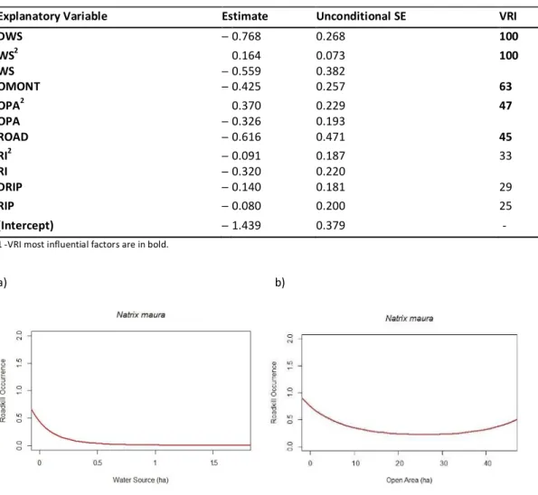
Model selection for the viperine snake N. maura resulted in 60 models (Table B4). Two highly influential variables were found, the Distance to Water Source (DWS) and Water Source (WS). Water source distance to roads was negatively associated to roadkill, as well as water source. In the first case, roadkill probability decreased as a water source became more distant from the road and in the second case the probability of a roadkill declined with increasing amount of water source (Figure 5). Open Montado, Open Area and Road Type were negatively associated to roadkill and still had a medium level influence in roadkill. The Roughness Index, Distance to
23
Riparian Gallery and Riparian Gallery showed a slight negative association to roadkill even though they were considered to have relatively low importance in the model set considered (Table 10).
TABLE 11-MODEL AVERAGING AND VARIABLE RELATIVE IMPORTANCE RESULTS FOR THE VIPERINE SNAKE Natrix
maura1.
Explanatory Variable Estimate Unconditional SE VRI
DWS ─ 0.768 0.268 100 WS2 WS ─ 0.164 0.559 0.073 0.382 100 OMONT ─ 0.425 0.257 63 OPA2 OPA ─ 0.370 0.326 0.229 0.193 47 ROAD ─ 0.616 0.471 45 RI2 RI ─ ─ 0.091 0.320 0.187 0.220 33 DRIP ─ 0.140 0.181 29 RIP ─ 0.080 0.200 25 (Intercept) ─ 1.439 0.379 -
1 -VRI most influential factors are in bold.
a) b)
FIGURE 7 – N. maura RELATIONSHIPS BETWEEN ROADKILL OCURRENCE AND a)WATER SOURCE OR b)OPEN
AREA.
A great number of models were generated for the rat snake M.
monspessulanus showing some model uncertainty (Table B5). M. monspessulanus
didn’t have strongly influential landscape variables related to area amount or distance. However, the Roughness Index was considered an important variable with a hump shaped curve, leading to increased roadkill up to intermediate levels (Figure 6). Road
24
Type was also an important variable and was negatively associated to roadkill (Table 12).
TABLE 12-MODEL AVERAGING AND VARIABLE RELATIVE IMPORTANCE RESULTS FOR THE RAT SNAKE Malpolon
monspessulanus1.
Explanatory Variable Estimate Unconditional SE VRI%
ROAD ─ 0.446 0.222 81 RI2 RI ─ 0.122 0.260 0.074 0.107 81 AGR ─ 0.108 0.091 38 DRIP ─ 0.091 0.088 33 SHR ─ 0.100 0.099 33 OMONT 0.093 0.094 30 HUM 0.069 0.073 29 RIP 0.004 0.091 20 OPA 0.001 0.102 20 (Intercept) 0.620 0.112 -
1 -VRI most influential factors are in bold.
25
D
ISCUSSION
Habitats influencing the movement of wildlife have been pointed as an influential characteristic for several vertebrates in determining roadkill locations (Clevenger, Chruszcz & Gunson 2003; Forman & Alexander 1998). And so the main objective of this study was to find connections and associated patterns between snake road crossing and snake habitat features in the roads surroundings that could influence roadkill events. For this purpose, landscape variables usually associated to snakes were used, plus a roughness index and a road type variable.
Since roadkill was recorded daily, one can expect that the endurance of snake carcasses on the pavement wasn’t much influenced whether by scavenging or by tire removing in the road, which most likely varies across regions and habitats (Degregorio
et al. 2011; Santos, Carvalho & Mira 2011). Indeed, Santos, Carvalho & Mira (2011) found that the persistence of snake carcasses in their study was around one day.
Most snake roadkill in the study area belonged to R. scalaris and M.
monspessulanus, which are both considered to be abundant species (Loureiro et al.
2010; Malkmus 2004; Salvador & Pleguezuelos 2002). These snakes have a diurnal activity and are active feeders, increasing their chance to encounter vehicles as these are more frequent during the day. Moreover, small mammals are often relatively abundant in road verges which may attract snakes searching for prey (Ruiz-Capillas, Mata & Malo 2013), also in the study area (Sabino-Marques & Mira 2011).Snakes with the least records were C. girondica, M. brevis and N. natrix. The first two species are nocturnal with relatively low abundances in Southern Portugal (Malkmus 2004), which may explain their low roadkill numbers. Finally, N. natrix is a rare species in its southern distribution limits, possibly due to the suboptimal habitat characteristics (Santos et al. 2002), so it can be expected for roadkill counts to be scarce.
In general terms, habitat cover was an important factor influencing snake community roadkill, although results may be biased towards the most abundant species in the data set. Montado, riparian galleries and human influenced area cover were linked to a higher probability of roadkill while shrubs, open areas and open
26
The Montado was the most important habitat cover influencing roadkill occurrence in snake community and second most important for R. scalaris. Even though other habitat types are important for snakes, a study has shown that oak woodland can be a crucial feature for Mediterranean snake communities and are often used in the hot and dry summer to avoid high temperatures (Filippi & Luiselli 2006). Also, the
Montado’s inherent diversity comprised of a mosaic of open area and woodland with
different tree density provides a structurally complex habitat most favoured by Mediterranean snake communities (Luiselli & Filippi 2006).
Snake community results also showed that riparian galleries cover and distance had a medium relative importance, whereas individual species showed that other environmental factors are relatively more important. Riparian galleries have been considered an habitat used by many snake species in the study area (Feriche 2009; Pleguezuelos & Brito 2008; Pleguezuelos 2009a; Pleguezuelos 2009b) and have already been suggested as the main cause in roadkill events of some of these species (Pleguezuelos 2009b, Santos 2009). Nevertheless, one suspects that perhaps other features associated to riparian galleries may be more important than cover or distance alone. Riparian galleries are usually long and thin and consequently have an extensive interface with adjacent habitats. The structural complexity that riparian galleries and their surroundings offer could be more meaningful than the riparian gallery alone, for example. In spite of most individual species showing a relative weak importance compared to other factors, the snake H. hippocrepis was an exception showing a higher roadkill probability at medium distances of riparian galleries, around 800 m.
The increase in human influenced cover increased roadkill probability for snake community and highly increased the chances of a roadkill happening for H. hippocrepis. Human influenced areas may be used by some snake species (R. scalaris, M.
monspessulanus), but to a lesser extent compared with H. hippocrepis which adapts
well to these environments (Feriche 2009). It seems that to a certain degree snakes have commensal liaisons with man activities, particularly with activities that directly favour rodent commensal populations (Malkmus 2004; Salvador & Pleguezuelos 2002). This may explain why this factor could be crucial in determining roadkill impact. As for
27
substitute and may even be encountered in more urban environments (Feriche 2009). Due to such a strong dependency on human structures, the expansion of human development and roads may greatly increase H. hippocrepis roadkill numbers, which is considered the most anthropophylic snake in the Iberian Peninsula (Salvador & Pleguezuelos 2002).
Conversely, agricultural land had medium importance in snake community roadkill, slightly increasing roadkill probability up to 20 ha of cover and greatly decreasing after this threshold. Agricultural land may offer favourable prey availability which explains why snakes may be killed while foraging for food in these areas. Results were similar for R. scalaris showing a slightly higher turning point at 25 ha of cover. In Portugal, R. scalaris is well adapted to traditional agricultural areas (with a mosaic pattern) where it can easily find places to hide and hunt animals, such as small mammals (Pleguezuelos 2009b). On the other hand, areas with intensified agriculture may be avoided because they are overly simplified and use too many pesticides.
In general terms, snake community had a lower probability of roadkill if the cover of open areas and open Montado was higher in the study area. A similar relationship was also shown for R. scalaris in open Montado. Even though open spaces may be attractive for basking, an increased extent of these areas may endanger snakes survival. Without the presence of hiding features snakes may be exposed to a greater risk of predation (e.g. birds of prey) and tend to avoid open terrain (Andrews, Gibbons & Jochimsen 2006). Open Montado as characterized in this study was composed of sparsely dispersed oak trees with less than 10% tree cover probably offering similar conditions of those present in open spaces.
Similarly, shrubs were also considered an important factor with a higher cover leading to lower roadkill for snake community and R. scalaris. Another study also found that snake mortality rate was lower in shrub habitat (Pragatheesh & Rajvanshi 2013). Perhaps the increase of shrub cover may lead to a structurally simplified habitat which can be considered unsuitable habitat for snakes. Actually, a Mediterranean snake species elsewhere was mostly associated to bushes when interspaced with open
28
grassy fields (Capula et al. 1997), so a similar behaviour could be expected from other Mediterranean snakes.
Indeed, the majority of terrestrial snake species (H. hippocrepis, M.
monspessulanus and R. scalaris) have a generalist behaviour occupying a wide variety
of niches (Malkmus 2004, Salvador & Pleguezuelos 2002). I suggest that the weak relationship that M. monspessulanus had with landscape factors may be due to being the most generalist species within the snake community. Fortunately, because of its huge plasticity and annual rising temperatures, it is less likely that roadkill is having a negative impact in its populations. Actually, an article has even mentioned an increase in populations for the studied area, as opposed to other snakes (Segura et al. 2007). We should expect the same trend for R. scalaris, however roadkill numbers in Portugal are very high and it is already suspected that population numbers are declining (Pleguezuelos 2009b). Consequently, roads are considered one of the biggest threats for this species.
Despite M. monspessulanus roadkill not showing influential landscapes, the roughness index was highly influential in determining roadkill. Likewise, snake community and terrestrial snakes studied were all associated to a roughness index with relatively high importance. Roadkill for snake community, R. scalaris and M.
monspessulanus was higher at medium levels of roughness and, in the case of H. hippocrepis, roadkill probability decreased as terrain got rougher. Taking into account
topographic features such as the roughness index or even other related features, as for instance slope or mean altitude, may be an important addition in finding spatial patterns that lead to snake roadkill, even more so for habitat generalist species.
Other parameters such as water source cover and distance were considered crucial factors in determining N. maura roadkill. Natrix maura is an aquatic species that is strongly dependent on aquatic features (Malkmus 2004, Santos 2009). Findings in our study verify this strong dependency, as N. maura roadkill showed a strong link to water source distance and cover. Here, this species may have no links to terrestrial habitats due to its aquatic habits and is quite adaptable too any kind of water source. It has even been seen in water sources altered by agricultural activities (Santos 2009),
29
even though mass population declines have been reported for polluted aquatic sources (Santos 2008).
Roads in the study area differ mostly because of their traffic volume. The national roads reach up to 10000 vehicles per day compared to municipal roads that have less than 4000 vehicles per day. We found that snakes mortality was higher in national roads than in municipal roads. Other studies have already discovered that snake roadkill is closely linked to traffic volumes (Colino-Rabanal & Lizana 2012; Pragatheesh & Rajvanshi 2013; Szerlag & McRobert 2006) adding support to our results. There are several reasons to why snake roadkill can be influenced by traffic patterns. Snake’s movement is slower in smoother road surfaces compared to other surfaces (Bonnet, Naulleau & Shine 1999; Roe, Gibson & Kingsbury 2006). Also, drivers have been reported to intentionally kill snakes due to aversion to them (Andrews, Gibbons & Jochimsen 2006; Row, Blouin-Demers & Weatherhead 2007). In Portugal, that is a common human behaviour.
This study has shown that landscape features can be used to identify spatial patterns in roadkill events. Another study involving snake spatial patterns in roadkill also showed this relationship (Pragatheesh & Rajvanshi 2013). More importantly, landscapes influencing roadkill differed from species to species revealing the importance of considering individual species in these studies. In brief, all the individual species seem to have distinctive landscape features that could certainly be influencing roadkill. To begin with, H. hippocrepis roadkill was higher with the increase of human influenced areas, then R. scalaris had a higher roadkill chance in landscapes that can be structurally more complex such as the Montado and possible traditional agricultural land, N. maura roadkill also was mostly associated to aquatic features and finally M.
monspessulanus roadkill was mostly influenced by terrain roughness and had a general
weak relationship with other landscape factors.
In the meantime, knowledge about the relationship between habitat and snake road mortality has a long way to go. Models can still include other variables that may improve our understanding on how habitat surroundings influence roadkill. For example, habitat selection in snakes is strongly correlated to prey’s resource
30
distribution (Luiselli & Filippi 2006). Also, some habitat characteristics such as rocky areas or shrub height were not incorporated in this study, possibly missing important snake habitat requirements.
Finally, models could also take into account snakes’ ecological differences such as age, sex or seasonal activity that can present shifts in habitat spatial use (Luiselli & Filippi 2006). Studies have already shown population declines in several snake species (Reading et al. 2010) and even for some snake species in the Iberian Peninsula, including Portugal (Pleguezuelos & Brito 2008; Santos 2008). Also, roads have been pointed as one of the main sources of mortality for several snake species in Portugal. Identifying major roadkill areas and related landscape features is an essential step to incorporate adequate management measures into road planning and mitigation implementation.
CONCLUDING REMARKS
This study revealed that roadkill events can be influenced by landscape factors. Individual species data showed that most important landscape features requirements were quite different between them, so important information could be missed when modelling snake species altogether.
If roadkill was more prominent in snake species that forage actively and have a diurnal behaviour, which agrees with another study (Bonnet et al. 1999), than it is still unclear how spatial patterns influence some of the less common snake species. Studying influences at the landscape level has shown important relationships with snake roadkill, but site specific characteristics may also have an important input in roadkill events. Variables selected at a finer scale may improve our knowledge about the role of habitat features in roadkill events. For example, spiny shrubs have been associated to the presence of snakes in the Mediterranean region as they function as a source of prey while also protecting against predators (Luiselli & Filippi 2006). Also, the height of shrubs or rocky features may be an important factor in determining habitat use, as H. hippocrepis and M. monspessulanus are found in areas with shrubs of low