Crop Yield Analysis of the Irrigated Areas of All Spatial Locations in Guntur District of AP.

(1)

Crop Yield Analysis of the Irrigated Areas of All Spatial

Locations in Guntur District of AP.

Ch. Mallikarjuna Rao

1

, Dr A. Ananda Rao

2

(Department of computer science and Engineering, Asso. Prof GRIET) (Department of Computer Science and Engineering, Professor, JNTUA)

ABSTRACT

Spatial data mining is a process to discover interesting and potentially useful spatial patterns embedded in spatial databases, which are voluminous in their sizes. Efficient techniques for extracting information from geo-spatial data sets can be of importance to various sectors like research, defense and private organizations for generating and managing large geo-spatial data sets. The current approach towards solving spatial data mining problems is to use classical data mining techniques. Effective analysis was done using the hybrid data mining techniques by mixing both clustering and classification techniques. In this paper crop yield of spatial locations of Guntur district were taken and studied using the hybrid technique.

Keywords

: geo-spatial data sets, hybrid data mining technique, clustering, classification, spatial locations

I. Introduction

Indian agriculture is known for more fluctuations in terms of crop yield, crop output and crop intensity. Despite growth in Technology and irrigation the production and income are highly instable [11]. Guntur district is located in the state of Andhra Pradesh. It is situated along the east coast of the Bay of Bengal. Its coastline is approximately 100 kilometers. It is the largest city and is the administrative center of the District. It has 57 mandals starting from Guntur, Pedakakani, Prathipadu, etc..to ending with Nizampatnam. Major crops are Cotton and Chillies. Analysis need to be done on the agriculture data sets which requires classical data mining techniques apart from statistical techniques. The data mining techniques[12] like classification, clustering and association are required to apply on the realistic data sets for analysis and conclusions on the agriculture crop yields [8, 9, and 10] of various seasons like Kharif and rubby. The following existing techniques are discussed along with proposed hybrid approach.

II. Literature Survey

K-Means clustering Algorithm:The k-means

algorithm [3] [Hartigan& Wong 1979] is the well known clustering technique used in scientific and industrial applications. Its name comes from centroid which is the mean of c of k clusters C. This technique is not suitable for categorical attributes. It is more suitable for numerical attributes. K-means[1] algorithm uses squared error criteria and is extensively used algorithm. The data is partitioned into K clusters (C1;C2; : : : ;CK), using this algorithm which are represented by their centers or means. The

mean of all the instances belonging to that cluster gives the center of each cluster.

The pseudo-code of the K-means algorithm is given by Fig.1. The algorithm begins with randomly selected initial set of cluster centers. Each instance is assigned to its closest cluster center for every iteration based on Euclidean distance calculated between the two. After thatre-calculate the cluster centers.

the instances number belonging to cluster k is denoted byNkand the mean of the cluster kis represented by µk.

There is a possibility for a number of convergence conditions. If the partitioning error is not reduced by the relocation of the centers the search will be stopped as it concludes that the present partition is locally optimal. Another stopping criteriais that if it exceeds a pre-defined number of iterations.

Input: S (instance set), K (no. of clusters)

Output: clusters

1: Initialize K cluster centers.

2: while termination condition is not satisfied do

3: Assign instances to the nearest cluster center. 4: Update cluster centers based on the assignment.

5: end while

Figure1. K-means Algorithm

This algorithm may be viewed as a gradient-decent procedure. In which it begins with random selection of an initial set number of K cluster-centers and iteratively updates by which error function will decrease. A rigorous proof of the finite convergence

(2)

of the K-means type algorithms is given in [4]. The complexity of T iterations of the K-means algorithm performed on a sample size of m instances, each characterized by N attributes, is: O(T * K * m * N). This linear complexity is one of the reasons for the popularity of the K- means algorithms. Even if the number of instances is substantially large (which often is the case nowadays), this algorithm is computationally attractive. Thus, the K-means algorithm has an advantage in comparison to other clustering methods (e.g. hierarchical clustering methods), which have non-linear complexity. Other reasons for the algorithm’s popularity are its ease of interpretation, simplicity of implementation, speed of convergence and adaptability to sparse data [5]. The Achilles heel of the K-means algorithm involves the selection of the initial partition. The algorithm is very sensitive to this selection, which may make the difference between global and local minimum. Being a typical partitioning algorithm, the K-means algorithm works well only on data sets having isotropic clusters, and is not as versatile as single link algorithms, for instance.

In addition, this algorithm is sensitive to noisy data and outliers (a single outlier can increase the squared error dramatically); it is applicable only when mean is defined (namely, for numeric attributes); and it requires the number of clusters in advance, which is not trivial when no prior knowledge is available. The use of the K-means algorithm is often limited to numeric attributes. The similarity measure for numeric attributes and categorical attributes differ in the first case take the square Euclidean distance; where as in second case take the number of mismatches between objects and the cluster prototypes.

Another partitioning algorithm, which attempts to minimize the SSE is the K-medoids or PAM (partition around medoids[2]). It is similar to the K-means algorithm. It differs with k-means mainly in representation of the different clusters. Each cluster is represented by the most centric object in the cluster, rather than by the implicit mean that may not belong to the cluster. This method is more robust than K-means algorithm even if there is noise and outliers. The influence of outliers is less. The processing of K-means is less costlierwhen compared to this. It is required to declare the number of clusters K for both the methods.It is not mandatory to use only SSE. Estivill-Castro (2000) analyzed the total absolute error criterion. He stated that it is better to summing up the absolute error instead of summing up the squared error. This method is superior in terms of robustness, but it requires more computational effort. The objective function is defined as the sum of discrepancies between a point and its centroid which

objective function, and is defined as the sum of squares of errors between the points and the corresponding centroids,

E( C ) = _{=1 �}_∈� � − � 2

It can be rationalized as log-likelihood for normally distributed mixture model. In Statistic it is extensively used. Therefore, it is derived from general framework of probability. Its iterative optimization has two versions. The first technique is similar to EM algorithm one of the Data mining technique. It has two-stepsof major iterations in which first time reassigns all the points to their nearest centroids, and second timerecompute centroids of newly formed groups. Iterations continue until a stopping criterion is achieved (for example, no reassignments happen). This version is known as Forgy.s algorithm [6] and has many advantages:

 It easily works with any -norm p L

 It allows straightforward parallelization[5]

 It is insensitive with respect to data ordering. If a move has a positive effect, the point is relocated and the two centroids are recomputed.

J48 algorithm:J48 [7]is the optimization of C4.5

algorithm and also animprovised versions of it.Its output result is a Decision tree which is of a tree structure. It has a root node, along with intermediate nodes apart from leaf nodes. Except Root node and leaf nodes every other node in the tree consistsof decision and which leads to our result. This tree divides the given space of a data set into areas of mutually exclusive. In this its data points are described by every area will have a label, a value or an action.The criterion of splitting is used to find which attribute makes the best split on the portion of tree of the training data set which in turn reaches to a particular node. Decision tree is formed by using the children attribute of the data set.

III. Proposed Approach

The raw data set was converted to the required format and then apply the data mining technique namely k-means clustering algorithm and then we get the new data set namely clustered data set. The classification technique J48 was applied on that clustered data set which results in hybrid model.

IV. Implementation of proposed

approach

(3)

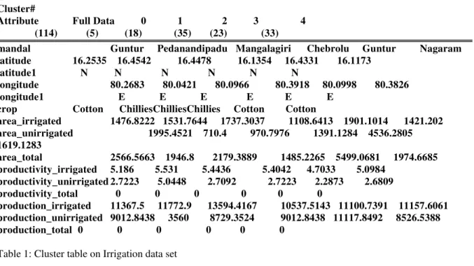
Discretization with 10 bins. Here full training set as the clustering model. The cluster table was represented by Table 1 and Cluster proximities were given by Table2. The cluster graph was shown below in Fig.2. The 5 clusters are shown in 4 different colors with instances on x-axis and mandals on y-axis. A hybrid model was developed and applied after applying K-means clustering.We took the J48 classification technique on the obtained clustered data set. The result was summarized as follows. It is with Minimum confidence is 0.25 and binary tree classifier. It also has same number of instances i.e.114 with 19 attributes. The attributes are Instance_number, mandal, latitude, latitude1, longitude, longitude1, crop, area_irrigated, area_unirrigated, area_total, etc. attributes. The J48 pruned tree is given below.

crop = Cotton

| latitude<= 16.37184

| pr

oductivity_unirrigated<= 3.239 | | latitude <= 16.340198

| | | production_irrigated<= 11367.5: cluster2 (35.0/1.0)

| | | production_irrigated> 11367.5: cluster1 (2.0)

| | latitude > 16.340198: cluster1 (15.0)

| productivity_unirrigated> 3.239: cluster0 (5.0)

The pruned tree in tree structure was shown in Fig.3 with crop as root node and clusters as leaf nodes. Correctly Classified Instances are 103 (90.351%) and Incorrectly Classified Instances are 11 (9.649%). Kappa statistic value is 0.8716.Kappa is a chance-corrected measure of agreement between the classifications and the true classes. It's calculated by taking the agreement expected by chance away from the observed agreement and dividing by the maximum possible agreement. A value greater than 0 means that your classifier is doing better than chance. The Kappa statistic is near to 1 so it is near to perfect agreement. Confusion Matrix: In the confusion matrix each column represents instances in the predicted class and each row indicates instances in actual class. These mining techniques were applied on various data sets.

V. Results & Analysis:

Initially k-means clustering technique was applied on Guntur Irrigation data set for analysis. Cluster 0: It was found that for the PedanandipaduMandal centroids of the latitude is

16.4542 N, Longitude is 80.0421 E with crop Chillies and area irrigated is 1531 area un-irrigated is 710 with area total is 1946 with highest productivity _irrigated 5.5 and productivity_unirrigated is 5. It also has highest production_irrigated and lowest Production_unirrigated with Productivity _total and Production_total as 0.

Cluster1 and 2 are also chillies as crop and production-irrigated is highest in cluster1with mandalsMangalagiri and chebrolu. Cluster 3 and 4 are with Mandals Guntur and nagaram and cotton is their crop. Cluster 3 is with highest area-irrigated and area_unirrigated. It also has highest area_total and production-unirrigated among the clusters. Confusion matrix shows that cluster 0 was classified accurately next to that was cluster 2. In cluster 1 out of 18 instances 23 were classified under cluster 2 and 1 was classified under cluster 3. Cluster3 and4 are not classified correctly. The values of TP rate and F-measure for cluster 0 are 1 indicates they are classified accurately. Cluster2 and 4 are also has TP rate and F-measure are almost 1,so classified almost accurately.

(4)

Cluster centroids: Cluster#

Attribute Full Data 0 1 2 3 4 (114) (5) (18) (35) (23) (33)

mandal Guntur Pedanandipadu Mangalagiri Chebrolu Guntur Nagaram

latitude 16.2535 16.4542 16.4478 16.1354 16.4331 16.1173

latitude1 N N N N N N

longitude 80.2683 80.0421 80.0966 80.3918 80.0998 80.3826

longitude1 E E E E E E

crop Cotton ChilliesChilliesChillies Cotton Cotton

area_irrigated 1476.8222 1531.7644 1737.3037 1108.6413 1901.1014 1421.202

area_unirrigated 1995.4521 710.4 970.7976 1391.1284 4536.2805

1619.1283

area_total 2566.5663 1946.8 2179.3889 1485.2265 5499.0681 1974.6685

productivity_irrigated 5.186 5.531 5.4436 5.4042 4.7033 5.0984

productivity_unirrigated 2.7223 5.0448 2.7092 2.7223 2.2873 2.6809

productivity_total 0 0 0 0 0 0

production_irrigated 11367.5 11772.9 13594.4167 10537.5143 11100.7391 11157.6061

production_unirrigated 9012.8438 3560 8729.3524 9012.8438 11117.8492 8526.5388 production_total 0 0 0 0 0 0

Table 1: Cluster table on Irrigation data set

(5)

Cluster-I Cluster-II Cluster-III Cluster-IV Cluster - V 5 1.682367 1 1.682367 1 1.682367 1 1.682367 1 1.682367 4 1.682367 3 2.236069 2 2.236069 3 2.236069 3 2.236069 2 1.682367 4 2.236069 4 2.236069 2 2.236069 4 2.236069 3 1.682367 5 2.236069 5 2.236069 5 2.236069 2 2.236069

Table2. Clusters along with their Proximities

The Confusion Matrix is given as below a bc d e <-- classified as

5 0 0 0 0 | a = cluster0 0 14 3 1 0 | b = cluster1 0 0 34 0 1 | c = cluster2 0 2 0 20 1 | d = cluster3

0 0 1 2 30 | e = cluster4

Fig4: Cotton irrigated area across years and mandals

Fig.5: Chillis irrigated area across years and mandals

-1000 0 1000 2000 3000 4000 5000 6000

1 3 5 7 9 11 13 15 17 19 21 23 25 27 29 31 33 35 37 39 41 43 45 47 49 51 53 55 57

Ir

ri

g

ate

d

A

re

a

Numbeer of Mandals

Cotton Irrigated area across years

_{Irrigated 2007-08}

Irrigated 2011-12

0 2000 4000 6000 8000

1 3 5 7 9 11 13 15 17 19 21 23 25 27 29 31 33 35 37 39 41 43 45 47 49 51 53 55 57

Irri

gat

e

d

ar

e

a

Number of Mandals

Chillies Irrigated area across years

(6)

Fig.6: Cotton and Chilli area in Hectors across Mandals of Guntur Best rules found:

1. longitude1=E 114 ==> latitude1=N 114 <conf:(1)> lift:(1) lev:(0) [0] conv:(0) 2. latitude1=N 114 ==> longitude1=E 114 <conf:(1)> lift:(1) lev:(0) [0] conv:(0)

3. productivity_total='All' 114 ==> latitude1=N 114 <conf:(1)> lift:(1) lev:(0) [0] conv:(0) 4. latitude1=N 114 ==>productivity_total='All' 114 <conf:(1)> lift:(1) lev:(0) [0] conv:(0) 5. productivity_total='All' 114 ==> longitude1=E 114 <conf:(1)> lift:(1) lev:(0) [0] conv:(0) 6. longitude1=E 114 ==>productivity_total='All' 114 <conf:(1)> lift:(1) lev:(0) [0] conv:(0)

7. longitude1=E productivity_total='All' 114 ==> latitude1=N 114 <conf:(1)> lift:(1) lev:(0) [0] conv:(0) 8. latitude1=N productivity_total='All' 114 ==> longitude1=E 114 <conf:(1)> lift:(1) lev:(0) [0] conv:(0) 9. latitude1=N longitude1=E 114 ==>productivity_total='All' 114 <conf:(1)> lift:(1) lev:(0) [0] conv:(0) 10. productivity_total='All' 114 ==> latitude1=N longitude1=E 114 <conf:(1)> lift:(1) lev:(0) [0] conv:(0) 11. longitude1=E 114 ==> latitude1=N productivity_total='All' 114 <conf:(1)> lift:(1) lev:(0) [0] conv:(0) 12. latitude1=N 114 ==> longitude1=E productivity_total='All' 114 <conf:(1)> lift:(1) lev:(0) [0] conv:(0) 13. productivity_irrigated='(4.967-5.5112]' 99 ==> latitude1=N 99 <conf:(1)> lift:(1) lev:(0) [0] conv:(0) 14. productivity_irrigated='(4.967-5.5112]' 99 ==> longitude1=E 99 <conf:(1)> lift:(1) lev:(0) [0] conv:(0) 15. productivity_irrigated='(4.967-5.5112]' 99 ==>productivity_total='All' 99 <conf:(1)> lift:(1) lev:(0) [0]

conv:(0)

16. longitude1=E productivity_irrigated='(4.967-5.5112]' 99 ==> latitude1=N 99 <conf:(1)> lift:(1) lev:(0) [0] conv:(0)

17. latitude1=N productivity_irrigated='(4.967-5.5112]' 99 ==> longitude1=E 99 <conf:(1)> lift:(1) lev:(0) [0] conv:(0)

18. productivity_irrigated='(4.967-5.5112]' 99 ==> latitude1=N longitude1=E 99 <conf:(1)> lift:(1) lev:(0) [0] conv:(0)

19. productivity_irrigated='(4.967-5.5112]' productivity_total='All' 99 ==> latitude1=N 99 <conf:(1)> lift:(1) lev:(0) [0] conv:(0)

20. latitude1=N productivity_irrigated='(4.967-5.5112]' 99 ==>productivity_total='All' 99 <conf:(1)> lift:(1) lev:(0) [0] conv:(0)

Fig.7 Association rules when minimum support = 0.85 and minimum confidence =0.9

Best rules found:

1. longitude1=E 114 ==> latitude1=N 114 <conf:(1)> lift:(1) lev:(0) [0] conv:(0) 2. latitude1=N 114 ==> longitude1=E 114 <conf:(1)> lift:(1) lev:(0) [0] conv:(0)

3. productivity_total='All' 114 ==> latitude1=N 114 <conf:(1)> lift:(1) lev:(0) [0] conv:(0) 4. latitude1=N 114 ==>productivity_total='All' 114 <conf:(1)> lift:(1) lev:(0) [0] conv:(0) 5. productivity_total='All' 114 ==> longitude1=E 114 <conf:(1)> lift:(1) lev:(0) [0] conv:(0) 6. longitude1=E 114 ==>productivity_total='All' 114 <conf:(1)> lift:(1) lev:(0) [0] conv:(0)

7. longitude1=E productivity_total='All' 114 ==> latitude1=N 114 <conf:(1)> lift:(1) lev:(0) [0] conv:(0) 8. latitude1=N productivity_total='All' 114 ==> longitude1=E 114 <conf:(1)> lift:(1) lev:(0) [0] conv:(0) 9. latitude1=N longitude1=E 114 ==>productivity_total='All' 114 <conf:(1)> lift:(1) lev:(0) [0] conv:(0) 10. productivity_total='All' 114 ==> latitude1=N longitude1=E 114 <conf:(1)> lift:(1) lev:(0) [0] conv:(0) 11. longitude1=E 114 ==> latitude1=N productivity_total='All' 114 <conf:(1)> lift:(1) lev:(0) [0] conv:(0)

0 2000 4000 6000 8000 10000 12000 G un tur P e da k ak an i P rat hi pa du Vat ti che ruk … P e da na nd ip … M an g al ag ir i T ad e pa ll i T hu ll ur u T ad ik o nd a A m ar av at hi S at te na pa ll i P e da k ur ap a … M e di k o nd ur u P hi ran g ipu r … M up pa ll a Kr o su ru A tc ha m pe t R aju pa le m B e ll am k o nd a N ar sa rao pe ta R o m pi che rl a Chi lak al u ri p … N ad e nd la E dl ap ad u Vi nu k o nd a N uz e nd la Ipu ru B o ll ap al li S av al y ap ur am P idu g ur al la M ac ha v ar am D ac he pa ll i Kar am pu di N e k ar ik al lu M ac he rl a Ve ldu rt hi D ur g i R e nt ac hi nt al a G ur az al a T e na li D u g g ir al a Ve m ur u Kol li pa ra Kol lur u P o nn ur T su nd ur u C he br o lu A m ar tal ur u B ap at la Kar lap al e m P .V. P al e m Kak um an u R e pa ll le N ag ar am B ha tt ipr o le C he ruk up al li N iz am pa tna m A re a in Hec to rs

Names of the Mandals

Cotton & Chilli area in Hec. across mandals

Total cotton area

(7)

VI.

Conclusion

There is a correlation between the cotton irrigated area of Irrigation 2007-08 and Irrigation2011-12 data and its value is 0.753871. There is a higher correlation between chillies irrigated area of Irrigation 2007-08 and Irrigation2011-12 data and its value is 0.869333.These analysis are specified in the results and analysis. Future scope of this hybrid approach can be extended to various agricultural spatial locations and also to various agricultural yields for effective analysis .

References

[1] PavelBerkhin, Survey of Clustering Data Mining Techniques, Accrue Software, Inc. [2] Kaufman, L. and Rousseeuw, P.J., 1987, Clustering by Means of Medoids, In Y. Dodge, editor, Statistical Data Analysis, based on the L1 Norm, pp. 405- 416, Elsevier/North Holland, Amsterdam. [3] Hartigan, J. A. Clustering algorithms. John

Wiley and Sons., 1975.

[4] Selim, S.Z., and Ismail, M.A. K-means-type algorithms: a generalized convergence theorem and characterization of local optimality. In IEEE transactions on pattern analysis and machine learning, vol. PAMI-6, no. 1, January, 1984.

[5] Dhillon I. and Modha D., Concept Decomposition for Large Sparse Text Data Using Clustering.Machine Learning.42, pp.143-175. (2001).

[6] FORGY, E. 1965. Cluster analysis of multivariate data: Efficiency versus interpretability of classification. Biometrics, 21, 768-780.

[7] Yugalkumar and G. Sahoo, Analysis of Bayes, Neural Network and Tree Classifier of Classification Technique in Data Mining using WEKA.

[8] Dr.T. V. RajiniKanth, Ananthoju Vijay Kumar, Estimation of the Influence of Fertilizer Nutrients Consumption on the Wheat Crop yield in India- a Data mining Approach, 30 Dec 2013, Volume 3, Issue 2, Pg.No: 316-320, ISSN: 2249-8958 (Online). [9] Dr.T. V. RajiniKanth, Ananthoju Vijay

Kumar, A Data Mining Approach for the Estimation of Climate Change on the Jowar Crop Yield in India, 25Dec2013,Volume 2 Issue 2, Pg.No:16-20, ISSN: 2319-6378 (Online).

[10] A. Vijay Kumar, “Estimation of the Influential Factors of rice yield in India” 2nd

International Conference on Advanced Computing methodologies ICACM-2013, 02-03 Aug 2013, ElsevierPublications, Pg.

No: 459-465, ISBN No: 978-93-35107-14-95

[11] Ramesh Chand, S.S. Raju, Instability in Andhra Pradesh agriculture -A Disaggregate Analysis, Agricultural Economics Research Review Vol. 21 July-December 2008 pp283-288.

[12] D. Hand, el al., Principles of Data Mining. Massachusetts: MIT Press, 2001.

AUTHORS

Ch.MallikarjunaRao

Received his B.Tech degree in computer

Science and engineering from Dr.Baba sahib AmbedkarMarathwada University, Aurangabad, Maharastra in 1998,and M.Tech Degree in Computer Science and Engineering from J.N.T.U Anantapur ,Andhrapradesh in 2007. He is currently pursuing his Ph.D degree from JNTU Ananthapur University, Andhra Pradesh. Currently he is working as Associate Professor in the department of Computer Science and Engineering of GokarajuRangaraju Institute of Engineering and Technology, Hyderabad, India.His research interest includes Data bases and data mining.

Dr. AnandaRaoAkepogureceived his B.

TechdegreeinComputerScience&Engineerin g from University of Hyderabad, Andhra Pradesh, India and M.Tech degree in A.I & Robotics from University of Hyderabad, Andhra Pradesh, India. He received Ph.D degree from Indian Institute of Technology Madras, Chennai, India. He is Professor of ComputerScience& Engineering Department and currently working as Principal of JNTUA College of Engineering, Anantapur, Jawaharlal Nehru Technological University, Andhra Pradesh, India. Dr. Rao published more than 100 publications in various National and International Journals/ Conferences. He received Best Research Paper award for the paper titled “An Approach to Test Case Design for Cost Effective Software Testing” in an International Conference on Software Engineering held at Hong Kong, 18-20 March 2009. He also received Best

Educationist Award for outstanding achievements in

the field of education by International Institute of Education & Management, New Delhi on 21st Jan. 2012. He bagged Bharat VidyaShiromani Award

from Indian Solidarity Council and

RashtriyaVidyaGaurav Gold Medal Award from