Deliverable 3.3 - Advanced Local Distribution Grid Monitoring / State-Estimation

(1)

THEME [ENERGY.2012.7.1.1] Integration of Variable Distributed

Resources in Distribution Networks

(Deliverable 3.3)

Advanced Local Distribution Grid

Monitoring / State-Estimation

Lead Beneficiary:

INESC Porto

(2)

List of Figures

Figure 1 - Structure of the state estimation module. ... 16

Figure 2 - Data flow chart of the load and state estimation ... 20

Figure 3 - Architecture of an autoencoder with a single hidden layer... 22

Figure 4 - Illustration of the POCS algorithm ... 23

Figure 5 - Illustration of the unconstrained algorithm ... 23

Figure 6 - Illustration of the constrained algorithm ... 24

Figure 7 - Flowchart of the main steps of the pseudo-measurements generation methodology ... 28

Figure 8 - Network partitioning in r non-overlapping areas ... 31

Figure 9 - Classification of buses and measurements in a multi-area power system. ... 32

Figure 10 - Classification of states and measurements in a multi-area power system. ... 35

Figure 11 - Illustrative example of distribution network multi-zone partitioning. ... 37

Figure 12 - Status of switching device k−l_{. ... 40}

Figure 13 - Modeling switching device associated with a branch. ... 40

Figure 14 - Modeling switching device associated with a generator or load. ... 40

Figure 15 - Voltage magnitude relative percentage errors (RPE) per network bus (Monday-Saturday)... 46

Figure 16 - Voltage magnitude relative percentage errors (RPE) per network bus (Sunday) ... 47

Figure 17 - Error Estimation Index (EEI) ... 48

Figure 18 - 2-norm Voltage Error ... 49

Figure 19 - 1-norm Power Flows and Injections Estimation Errors ... 50

Figure 20 - 2-norm Power Flows and Injections Estimation Errors ... 50

Figure 21 - Infinity-norm power flows and injections estimation errors ... 51

Figure 22 - Ratio of power flows and injections estimation errors ... 52

Figure 23 - Convergence KPIs ... 52

Figure 24 - True and estimated active bus injections (single bad data at generation bus 121). ... 54

Figure 25 - True and estimated reactive bus injections (single bad data at generation bus 121). ... 54

Figure 26 - True and estimated node voltage magnitudes (single bad data at generation bus 121). ... 55

Figure 27 - True and estimated node voltage angles (single bad data at generation bus 121). ... 55

Figure 28 - True and estimated active bus injections (single bad data at load bus 8). ... 56

Figure 29 - True and estimated reactive bus injections (single bad data at load bus 8). ... 56

Figure 30 - True and estimated node voltage magnitudes (single bad data at load bus 8). ... 57

Figure 31 - True and estimated node voltage angles (single bad data at load bus 8). ... 57

Figure 32 - True and estimated active bus injections (bad data at generation bus 380 and load bus 324). ... 58

(5)

Figure 33 - True and estimated reactive bus injections (bad data at generation bus 380

and load bus 324). ... 58

Figure 34 - True and estimated node voltage magnitudes (bad data at generation bus 380 and load bus 324). ... 59

Figure 35 - True and estimated node voltage angles (bad data at generation bus 380 and load bus 324). ... 59

Figure 36 - Case 1: Division into 3 areas (R-220 (1) & R-260 (2)) ... 60

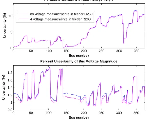
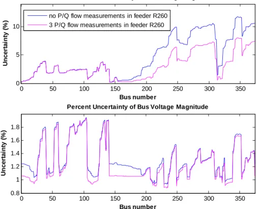
Figure 40 - Uncertainty of magnitude and angle of estimated bus voltages (Case 1). ... 66

Figure 44 - Typical Portuguese LV network of 100 kVA considered... 76

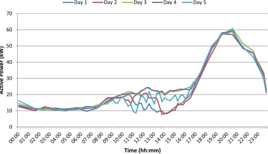
Figure 45 - Example of the active power measured at the substation level for the first 5 days ... 78

Figure 46 - Microgeneration production diagrams obtained from a real meteorological station ... 79

Figure 47 - Absolute error of the injected active power for each scenario (MW) ... 87

Figure 48 - Absolute error of the injected reactive power for each scenario (Mvar) ... 88

Figure 49 - Absolute error of the voltage magnitude for each scenario (p.u.) ... 88

Figure 50 - Pseudo-measurements and real values of injected active power for the entire evaluation set, for each scenario (MW) ... 89

Figure 51 - Pseudo-measurements and real values of injected reactive power for the entire evaluation set, for each scenario (Mvar) ... 90

Figure 52 - Pseudo-measurements and real values of voltage magnitude for the entire evaluation set, for each scenario (p.u.) ... 93

Figure 53 - Portuguese MV network used as test case. The orange circle identifies the only one MV/LV secondary substation without the capability of transmitting data in real-time considered – substation number 0426 (Casinha-Sul) ... 96

Figure 54 - Absolute error of the voltage magnitude obtained, for all MV/LV secondary substations, using the pseudo-measurements generated in scenario 1 (p.u.) ... 98

Figure 59 - Absolute error of the voltage magnitude obtained, for all MV/LV secondary substations, using no pseudo-measurements (p.u.) ... 101

(6)

Figure 60 - Absolute error of the voltage magnitude obtained, for the MV/LV secondary substation without the capability of transmitting data in real-time considered, with and without using the pseudo-measurements generated in each scenario (p.u.) ... 101 Figure 61 - Representation of the voltage magnitude for the considered period: real values and estimated ones using the pseudo-measurements generated in scenario 1. The pseudo-measurement of the voltage magnitude used is also shown (p.u.) ... 102 Figure 62 - Representation of the voltage magnitude for the considered period: real values and estimated ones using the pseudo-measurements generated in scenario 2. The pseudo-measurement of the voltage magnitude used is also shown (p.u.) ... 102 Figure 63 - Representation of the voltage magnitude for the considered period: real values and estimated ones using the pseudo-measurements generated in scenario 3. The pseudo-measurement of the voltage magnitude used is also shown (p.u.) ... 103 Figure 64 - Representation of the voltage magnitude for the considered period: real values and estimated ones using the pseudo-measurements generated in scenario 4. The pseudo-measurement of the voltage magnitude used is also shown (p.u.) ... 103 Figure 65 - Representation of the voltage magnitude for the considered period: real values and estimated ones using the pseudo-measurements generated in scenario 5. The pseudo-measurement of the voltage magnitude used is also shown (p.u.) ... 104 Figure 66 - Representation of the voltage magnitude for the considered period: real values and estimated ones using no pseudo-measurements (p.u.) ... 104 Figure 67 - Representation of the voltage magnitude for all MV/LV secondary substations: real values and estimated ones with and without using the pseudo-measurements

generated in scenario 3 (p.u.) ... 105 Figure 68 - Voltage magnitude relative percentage errors (RPE) per network substation (with and without using pseudo-measurements) ... 109 Figure 69 - Distribution of the voltage magnitude relative percentage errors (RPE) per network substation (with using pseudo-measurements generated in scenario 1) for the entire considered week ... 110 Figure 70 - Distribution of the voltage magnitude relative percentage errors (RPE) per network substation (with using pseudo-measurements generated in scenario 2) for the entire considered week ... 110 Figure 71 - Distribution of the voltage magnitude relative percentage errors (RPE) per network substation (with using pseudo-measurements generated in scenario 3) for the entire considered week ... 111 Figure 72 - Distribution of the voltage magnitude relative percentage errors (RPE) per network substation (with using pseudo-measurements generated in scenario 4) for the entire considered week ... 111 Figure 73 - Distribution of the voltage magnitude relative percentage errors (RPE) per network substation (with using pseudo-measurements generated in scenario 5) for the entire considered week ... 112 Figure 74 - Distribution of the voltage magnitude relative percentage errors (RPE) per network substation (without using pseudo-measurements) for the entire considered week... 112 Figure 75 - Production and Transmission System of Rhodes ... 118

(7)

Figure 76 - Substation Gennadiou ... 119

Figure 77 - Feeder R-220 ... 120

Figure 78 - Feeder R-260 ... 121

(8)

List of Tables

Table 1 - State estimation approaches. ... 18

Table 2 - Statistical results for weekly state estimation simulations. ... 47

Table 3 - Measurement configuration for each test case ... 62

Table 4 - CPU time for Case 0 ... 63

Table 8 - CPU for Case 4 ... 64

Table 9 - Comparison of maximum CPU times for the test cases ... 64

Table 10 - Description of test cases for meter placement ... 65

Table 11 - True, assumed and estimated status of switching devices for cases 1 to 3 ... 69

Table 12 - True, assumed and estimated status of switching devices for cases 4 to 8 ... 70

Table 13 - True, assumed and estimated status of switching devices for cases 9 to 13... 71

Table 14 - Normalized residual test for Cases 1 to 5 ... 72

Table 17 - Normalized residual test for Case 10... 75

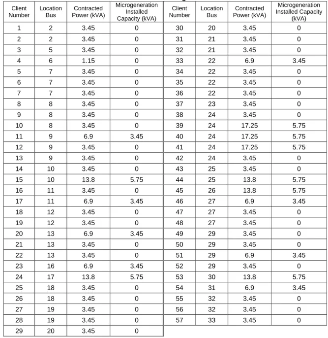
Table 19 - Consumers and microgeneration distribution ... 77

Table 20 - Set of SM with the capability of transmitting data in real-time with more influence in pseudo-measurements generation performance ... 81

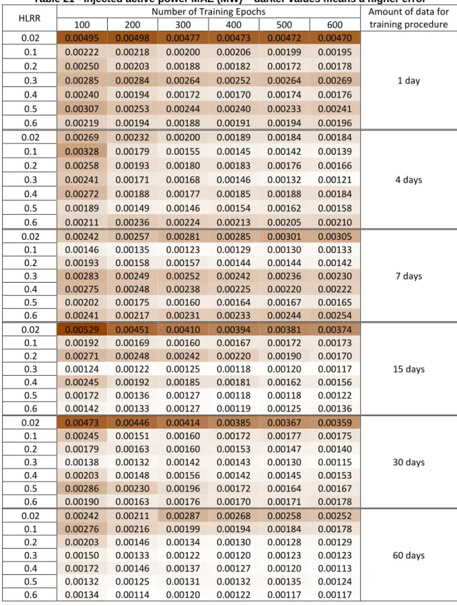
Table 21 - Injected active power MAE (MW) – darker values means a higher error ... 82

Table 22 - Injected reactive power MAE (Mvar) – darker values means a higher error ... 83

Table 23 - Voltage Magnitude (p.u.) – darker values means a higher error ... 84

Table 24 - Hidden layer reduction rates and its hidden layer neurons correspondence, for the described scenario ... 85

Table 25 - Number of SM and its location for each created scenario ... 87

Table 26 - Pseudo-measurements MAE for each scenario ... 88

Table 27 - Training and running times for each created scenario... 94

Table 28 - Voltage magnitude MAE obtained with and without using the pseudo-measurements generated in each scenario (p.u.) ... 101

Table 29 - Nominal apparent power at load and generation nodes of feeder R220 ... 123

Table 30 - Zero injection nodes of feeder R220 ... 124

Table 35 - Types and electric parameters of overhead cables ... 128

Table 36 - Line data for feeder R220 (on 5 MVA base) ... 129

(9)

(10)

List of Acronyms and Abbreviations

AANN Auto-associative neural networks

AMI Advanced Metering Infrastructure AMM Advanced Metering Management CB Circuit Breaker

CC Control Centre CL Controllable Load DG Distributed Generation

DMS Distribution Management Systems DoW Description of Work

DSE Distribution State Estimation DSM Demand Side Management DSO Distribution System Operator DT Distribution Transformer

DTC Distribution Transformer Controller

EB Smart Meter

EMS Energy Management Systems

EPSO Evolutionary Particle Swarm Optimization GPS Global Positioning Systems

HLRR Hidden Layer Reduction Rate HMI Human-Machine Interface

HV High Voltage

IED Intelligent Electronic Device

LV Low Voltage

MV Medium Voltage

PCA Principal Component Analysis PMU Phasor Measurement Units POCS Projection Onto Convex Sets PV Photovoltaic Unit

(11)

RPROP Resilient Back-Propagation RTU Remote Terminal Unit

SCADA Supervisory Control and Data Acquisition SAS Substation Automation System

SE State Estimation

SM Smart meter

SSC Smart Substation Controller TSO Transmission System Operator

WF Wind Farm

(12)

AUTHORS:

Authors Organization Email

Jorge Pereira INESC Porto jpereira@inesctec.pt

Pedro Pereira Barbeiro INESC Porto pedro.p.barbeiro@inesctec.pt Henrique Teixeira INESC Porto henrique.s.teixeira@inesctec.pt

George Korres ICCS/NTUA gkorres@cs.ntua.gr

Xygkis Themistoklis ICCS/NTUA txiggs@hotmail.com Manousakis Nikolaos ICCS/NTUA manousakis_n@yahoo.gr Despina Koukoula ICCS/NTUA kdespina@power.ece.ntua.gr Panayotis Moutis ICCS/NTUA Pmoutis@power.ece.ntua.gr

Access: Project Consortium European Commission

Public X

Status: Draft version

Submission for Approval

(13)

1 Introduction

Description of the Task 3.3 “Advanced Local Distribution Grid Monitoring / State-Estimation” from the DoW (section 3.3.1)

Task 3.3 Advanced local distribution grid monitoring / state-estimation (Task leader: INESCP; ICCS) In this task, a robust approach to distribution state estimation will be developed with enough robustness to face lack of information collected from the smart meters or RTU located in the grid by using additional historical information stored in the system data base.

The following sub-tasks are envisaged:

• Sub-Task 3.3.1 – MV grid topology identification using multiple data sources (including namely the information collected from the smart metering support infrastructure)

The correct network topology will be identified by using status information of switching devices, real-time analogue measurements, pseudo measurements (forecasted or historical load data) and virtual measurements (zero injection nodes, operational constraints of open/closed switching devices, radiality constraints), and any available information from smart metering equipment. A generalized probabilistic optimization formulation will be used to identify network topology. Statistical tests will be made to identify inconsistencies among analogue and digital information and eliminate any bad data. Opening switching operations may cause network splitting and the state variables in all the resulting islands will be determined by adding appropriate operating constraints in the state estimation formulation. The proposed approach will eliminate the need of repeated state estimation runs for alternative hypothesis evaluation.

• Sub-Task 3.3.2 – MV grid state estimation in distribution grids using smart metering information Different state estimation formulations will be investigated for the best exploitation of the information from Advanced Metering Infrastructure (AMI) and Smart Global Positioning Systems (GPS) and synchronized Phasor Measurement Units (PMU) devices. Smart meters connected to a node, make time synchronized measurements of the active and reactive loads at predefined time intervals. These measurements will be transmitted to a database server periodically. This makes sure that the state estimator will have, at least, previous day’s measurements of all the loads.

To facilitate the computation burden of the enormous volumes of data produced from the smart meters and the load forecasting algorithms, distributed processing will be implemented, by dividing the network into several zones. The zones will perform local estimation that leads to global estimation through information exchange, coordination and communication among them.

To assure accurate distribution voltage estimations and minimize the estimated voltage uncertainty, identification of the minimum number and location of additional voltage and current sensors in the network is needed.

In each of these subtasks, a pre-prototype of the software tool will be developed and validated. A specification of the database and data communications requirements will be established and will feed the operational phase.

The advanced local distribution grid monitoring / state estimation will be based at the top level of the system architecture (central systems) and also at the HV/MV substation having as input information gathered from lower levels of the architecture.

(14)

Hence, equipment deployed must not only have a great deal of processing capability but also be able to collect data from local sensors. Also, an adequate and flexible communication link must be guaranteed. For this functionality, several data acquisition points are required so that enough redundancy is assured to make the state estimation function converge and have accurate results.

The main objective of the state estimation (SE) functionality is to find the values for a set of variables (states) that adjust in a more adequate way to a set of network values (measurements) that is available in real-time [1], [2]. The state variables are such that all the other network variables can be evaluated from them, and the operation state is obtained. The calculation of the state variables considers the physical laws directing the operation of electrical networks and is typically done adopting some criteria. The Distribution State Estimation (DSE) is implemented at the functional level of the HV/MV primary substation and only the MV level state variables are calculated [3]–[7]. It is assumed that the state estimation functionality will be installed at the central management level, i.e., at the SCADA/DMS. The following issues should be considered in distribution networks:

• Instrumentation: no (or only a few) sensors in the distribution networks.

• Algorithmic: long radial feeders with heterogeneous lines and cables may result in ill conditioned matrices.

• Large number of nodes: long calculation times.

• Active and reactive power cannot be decoupled: decoupled transmission state estimation algorithms cannot be applied.

(15)

2 MV grid state estimation in distribution grids using

smart metering information (sub-task 3.3.2)

In order to derive consistent and qualified state estimates, it is necessary to use all the information available for the network and not only real-time measurements, because their availability is very limited. Therefore, the DSE functionality includes information coming from different sources, namely: AMI, DTC acting as Remote Terminal Units (RTUs), and Phasor Measurement Units (PMUs) synchronized by the Global Position System (GPS) signal, if available [8]–[11]. Smart meters (EBs) connected to LV nodes can make time-synchronized measurements of active (P) and reactive (Q) loads, as well as voltage magnitudes, at predefined time intervals (usually every 15 minutes). These measurements are transmitted to a database server periodically (for instance, daily). This ensures that the DSE will have, at least, measurements from the previous day of all the loads [6].

Based on these measurements a set of pseudo-measurements will be generated and used together with near real-time information, for instance from distributed generators (DG) [6], to make the network fully observable and guarantee an adequate degree of redundancy for running the state estimator. This can be accomplished by an autoregressive load estimation model [12], which utilizes previous day metered LV consumption data as well as same day dependent variables, such as temperature, day type (weekday or weekend), humidity, etc. The upstream MV/LV substation load will be estimated by aggregating all the downstream LV loads, using an expert system trained specifically for this purpose [13], [14]. This expert system will be located at the central management level, where historical information is available.

The MV/LV substations that require generation of these pseudo-measurements, are those without DTC or substations where the transmission of real time DTC measurements has failed. When a MV/LV substation has a DTC with measurements that are available in real-time, the generation of pseudo-measurements is not necessary.

The structure of the state estimation module is shown in Figure 1.

The following input information should be available to state estimator: network parameters and configuration (topology) as well as analog measurements, such as actual

(telemetered) measurements subject to errors, due to metering inaccuracies,

communication system etc (active and reactive power flows, branch currents, active and reactive injections - loads and generations - node voltage magnitudes, statuses of switching devices, and position of transformer taps), pseudo measurements subject to errors (forecasted load injections or manually entered measurements of any type), and

virtual measurements which contain no error (zero injections at network nodes that have

neither load nor generation, zero voltage drops at closed switching devices, and zero active and reactive power flows at open switching devices).

(16)

Figure 1 - Structure of the state estimation module.

After the execution of the SE algorithm, the voltage magnitudes and phase angles of the network nodes are estimated. The following output information is provided:

• Voltage magnitudes and phase angles at all nodes.

• Active and reactive injected power at each generation and load node.

• Active and reactive power flows at both sides of each line, transformer, and switch. • Current flows at both sides of each line, transformer, and switch.

• Detection and removal of bad and conflicting data.

• Status of the switching devices with unknown or wrong status. • Critical and noncritical measurements.

• Performance metrics and confidence indices for the computed solution.

2.1 State Estimation Algorithm

Although distribution systems are unbalanced in nature, in order to avoid modelling complexities, the network is assumed to be balanced and the single phase equivalent network model is considered for power flow and state estimation analysis. In this research, the following nonlinear measurement model is used:

z = h(x)+ e (1)

where z is the measurement vector, h(x) is the vector of nonlinear functions relating

(17)

(magnitudes and phase angles), and e is the vector of measurement errors. The class of

estimators discussed in this section are based on the maximum likelihood theory and rely on a priori knowledge of the distribution of the measurement error (normally distributed, with E (e)= 0 and E (ee )= R = diag(T σ_i2), where σ_i2 is the variance of the ith

measurement error). A node is arbitrarily selected as the reference node and its voltage angle is set to zero.

Measurements can be classified as critical (nonredundant) and noncritical

(redundant). A critical measurement is the one whose elimination from the measurement

set makes the network unobservable [2]. Critical measurements have zero residuals and therefore their errors cannot be detected. If these measurements are inaccurate no action can be taken. Noncritical measurements have nonzero residuals, allowing detection and possibly identification of their errors. A minimally dependent set of measurements has the property that elimination of any measurement from this set, makes the remaining measurements critical. All the measurements of a minimally dependent set have equal absolute values of their normalized residuals [30]. As a consequence, gross error on one or more measurements of a minimally dependent set can be detected but not identified. The critical measurements and minimally dependent sets of measurements are determined by method [30]. Since the measurement redundancy is low in distribution networks, few critical measurements and minimally dependent sets may occur, making the error filtering process rather difficult. This is the reason why forecasted load (pseudo) measurements should be as accurate as possible.

Since distribution systems have limited or no measurement redundancy, the suitability of the state estimation algorithms that have been suggested for transmission systems needs further investigation [5]. The available measurements are predominantly of pseudo type (statistical in nature), so the performance of SE should be based on some statistical measures, such as bias, consistency and quality. These statistical measures are explored by investigating three of the most common transmission system state estimation approaches [5] with regard to their suitability for the DSE problem under stochastic behaviour of the measurements and limited or no redundancy [3], [4].

The problem is to find an estimate xˆ of the state vector which minimizes the

following objective function:

= =

_∑

m i i J x r 1 ( )

ρ

( ) (2)

where r_i: N(0,1) is the weighted residual of the ith measurement:

− = i i i i z h x r ( ) σ (3)

Table 1 summarizes the adopted SE approaches. The different estimators can be characterized based on the choice of the ρ function.

(18)

Table 1 - State estimation approaches.

Approach

ρ

( )ri Solution method

Weighted Least Squares

(WLS) ri

2

1

2 Newton iterative

Weighted Least Absolute

Value (WLAV) ri

Linear Programming (LP) or Interior Point (IP)

Schweppe-Huber Generalized-M (SHGM)  ≤    ₋  i i i i i i r r w w r w 2 2 2 1 if 2 1 otherw ise 2 α α α

where w_i is the iteratively

modified weighting factor and

α

is a tuning parameter

Iteratively Reweighted Least Squares (IRLS)

The performance evaluation of the above SE techniques have showed that WLAV and SHGM methodologies cannot be applied to distribution systems [5]. The WLS method gives consistent and better quality performance when applied to distribution systems. Hence, WLS is found to be the suitable solver and is used in this project.

The solution xˆ can be found by the normal equations (NE) iterative procedure as

follows: − ∆ = ∆ k k T k k G x( ) x H (x )R 1 z (4) where, ∆ =k k+ − k

x x 1 x , ∆ = −zk z h x( k),H =∂ ∂h x is the Jacobian matrix evaluated at

= k

x x , G =H TR−1H is the gain matrix evaluated at x=xk, and k is the iteration

index.

2.2 Required Data for State Estimation Execution

The SE algorithm will run at pre-defined time intervals (i.e. every 15 minutes or every hour). Accurate load models are critical for state estimation. Innovative techniques will identify load models and load compositions (i.e. demand profiles), using standard available measurement data at network buses, individual demand component signatures and general information about demand composition.

Load modeling in the distribution network will have the following characteristics: • For unmeasured nodes, load profiles will be developed for each type of customer

(19)

energy bill data. Historical samples obtained for different seasons, days and times, will be stored separately for different load types (residential, industrial and commercial). • For measured nodes, the consumed P, Q power will be provided.

It is assumed that domestic smart meters connected to a node, take synchronized measurements of active and reactive consumption of the loads at predefined time intervals. These measurements are transmitted to a database server periodically, i.e. AMR data in the PCC’s MV distribution system for the current day are transmitted from 00.00 hrs to 06.00 hrs of the next day. In any case, state estimator will have the previous day’s measurements of all the loads. The proposed state estimator will estimate reliably the node voltages of a distribution network by using the previous day’s measurements (while considering whether the day is a weekday, Saturday and Sunday). The AMR meters installed at distributed generators (DG) will measure net P, net Q and V at predefined time intervals and communicate immediately to the server. The SE will also read P/Q consumption of the loads connected to each transformer which will summed up (as the measurements are time synchronised) to calculate the load of the transformer (and the node). The previous day’s loads of the nodes and near real-time power measurements from distributed generators will be used as power injection measurements.

Summarizing, the required data for state estimation execution are shown below.

LV network

− P/Q power consumption and V magnitude at every LV load bus

− P power production and V magnitude at every LV production bus.

MV network

− P/Q power consumption at MV consumption bus, if available

− P/Q power production and V magnitude and phase at MV production bus, if available.

− P/Q power flow in the MV lines with RTU or PMU. MV/LV (secondary) substations

P/Q power consumption, V magnitude and/or I magnitude and power factor, in the primary or secondary of the transformer, if available. HV/MV (primary substation) P/Q power consumption, V magnitude and/or I

magnitude and power factor, in the primary or secondary of the transformer, if available. These measurements could also be available for each MV feeder;

The transmission frequency for each data level is shown below.

Past data of the LV network It should be available once a day with 24 hours of delay (i.e., from d-1).

(20)

network DTC) should be available every 15 minutes with a maximum delay of 1 minute.

MV network It should be available in real time (e.g., on a 1 minute time basis).

Figure 2 - Data flow chart of the load and state estimation

A general framework for the combined simulation of load and state estimation is presented in Figure 2. The load estimation algorithm is using data provided by LV or MV smart meters. It deploys a simple time series model [8] using basic class-specific load curves associated to each consumer type (e.g. domestic, commercial etc.) to improve the accuracy of individual customer load estimates. Load estimates can be obtained hourly, half-hourly or less. Then, all individual load estimates are aggregated, based on topology and connectivity data, to extract load estimates per MV/LV distribution transformers. These values are treated as pseudo-measurements and used as inputs to state estimation algorithm along with (near) real-time data collected from other points of the power network. Time delay in data transmissions from smart meters to data management centers is a parameter which affects significantly the load estimation algorithm performance.

(21)

2.3 Pseudo-measurement generation with autoencoders

In order to derive consistent and qualified state estimates, it is necessary to use all the information available for the network and not only real-time measurements, because their availability is very limited. Smart meters (EBs) connected to LV nodes can make time-synchronized measurements of active (P) and reactive (Q) loads, as well as voltage magnitudes (V), at predefined time intervals (usually every 15 minutes). These measurements are transmitted to a database server periodically (for instance, daily).

Based on these “historical” measurements and with some real-time information from LV network, a set of pseudo-measurements for the secondary substations will be generated and used together with near real-time information for MV network, to make the network fully observable and guarantee an adequate degree of redundancy for running the state estimator at the MV network. This can be accomplished by an Auto-associative neural networks (AANN) or autoencoders [14], which utilizes historical metered LV data to be properly trained. The pseudo-measurements generation consists of running the autoencoder, already trained, incorporating an optimization procedure for reconstructing the missing variables of the secondary substations [15].

This expert system will be located at the central management level, where historical information is available.

The MV/LV substations that require generation of these pseudo-measurements, are those without DTC or substations where the transmission of real time DTC measurements has failed. When a MV/LV substation has a DTC with measurements that are available in real-time, the generation of pseudo-measurements is not necessary.

2.3.1 The Autoencoder Concept

Auto-associative neural networks (AANN) or autoencoders are feedforward neural networks that are built to mirror the input space S in their output. The size of the output layer is the main difference between an autoencoder and a traditional neural network – in an autoencoder the size of its output layer is always the same as the size of its input layer. Therefore, an autoencoder is trained to display an output equal to its input. This is achieved through the projection of the input data onto a different space S’ (in the middle layer) and then re-projecting it back to the original space S. In other words, the first half of the autoencoder approximates the function f that encode the input space to the space compressed S’ while the second half approximates the inverse function f-1that projects back the set of values in space S’ to the original space S. The detailed mathematical formulation can be found in [16]. With adequate training, an autoencoder learns the data set pattern and stores in its weights information about the training data manifold. The

(22)

typical architecture of an autoencoder is a neural network with only one middle layer – Figure 3 This simple architecture is frequently adopted because networks with more hidden layers have proved to be difficult to train [17], although allowing increasing accuracy. An autoencoder with one hidden layer and linear activation functions performs the same basic information compression from space S to space S’ as Principal Component Analysis (PCA) [18]. With nonlinear activation functions and multiple layers, autoencoders chart the input space on a non-linear manifold in such a way that an approximate reconstruction is possible with less error [19]. Plus, PCA does not easily show how to do the inverse reconstruction, which is straightforward with autoencoders.

Figure 3 - Architecture of an autoencoder with a single hidden layer

There is no a priori indication of an adequate hidden layer reduction rate (measured as the ratio between the number of neurons in the smallest middle layer and the number of neurons in the input/output layer) to be adopted. This decision on the reduction rate is dictated in present-day practice by trial and error and by characteristics of the problem.

Autoencoders with thousands of inputs have been proposed for data or image compression, using the signals available in the middle layer, which maps the input to a reduced dimension space. Reconstruction is then performed using the second half of the autoencoder [20-22].

Once the autoencoder is trained, if an incomplete pattern is presented, the missing components may be replaced by random values producing a significant mismatch between input and output. Typically three different approaches can be followed in order to find the missing values on the way to minimize that error (convergence is reached). The approach called Projection Onto Convex Sets (POCS) [23] consists basically in iteratively reintroducing the output value in the input such that it will converge to a value that minimizes the input-output error (Figure 4). This convergence method uses alternating linear projections on the input and output space to converge to the assumed

(23)

missing values. The two other approaches are based on an optimization algorithm in order to discover the values that should be introduced in the missing components such that the input-output error becomes minimized. In the process denoted unconstrained search, the convergence is controlled only by the error on the missing signals (Figure 5), whereas in the constrained search it is controlled by the error on all the outputs of the autoencoder (Figure 6). Any of these optimization procedures may be used, but according to some related works in the state estimation area [14, 24], constrained search appears to the most suitable method to search a missing signal.

Figure 4 - Illustration of the POCS algorithm

(24)

Figure 6 - Illustration of the constrained algorithm

Autoencoders are frequently applied in areas related with pattern recognition and reconstruction of missing sensor signals [20, 25]. However, their application in the power systems area is not very common. In [14] one can find the proposal of offline trained autoencoders for recomposing missing information in the SCADA of Energy/Distribution Management Systems (EMS/DMS). Also in [24], a model for breaker status identification and power system topology estimation is presented. More recently, in [26] is proposed a concept of transformer fault diagnosis and in [15] one can find an innovative method to perform state estimation in distribution grids, both applications using autoencoders.

2.3.2 Methodology

In the present work it is expected to estimate the MV network operation state using data of the real-time measurements available on the MV network and also pseudo-measurements and/or other pseudo-measurements taken from smart meters and other equipment installed in the LV network.

In order to turn the MV network observable will be used a pseudo-measurement generation method for MV/LV secondary substation without real-time measurements. The LV measurements will be considered to generate pseudo-measurements for the upstream MV/LV substation load, which aggregates all downstream LV loads and LV generation. This will be done using an autoencoder properly trained and located at the central management level or at DTC level, where historical information is available.

A constrained search approach is applied for finding the missing signals (see Figure 6). In the context of this approach, to generate pseudo-measurements for the MV/LV secondary substation without real-time measurements, missing signals have to be the active and reactive injected power and also the voltage magnitude value, all calculated at the bus of the secondary level of the correspondent substation.

(25)

Within the constrained search approach, the optimization algorithm used to reconstruct the missing signals was a meta-heuristic method called Evolutionary Particle Swarm Optimization (EPSO). The EPSO algorithm has been successfully applied already in several problems in the power systems area [27-29]. The fitness function of the EPSO was defined to minimize the square error between the input and the output of the autoencoder.

2.3.2.1 Historical Data

An effective pseudo-measurements generation through the use of autoencoders requires inevitably a large historical database, which needs to contain data about the variables that are passed to the autoencoder (missing signals and measurements recorded). Additionally, the amount of data for each time instant/operating point should be available in enough number. This is crucial for a successful and effective training process since it is what enables the autoencoder to learn the necessary patterns/correlations between the electrical variables of a given network. There is no rule of thumb regarding the quantity of data in the historical database. However, it is known that few or too much data will lead to an inaccurate autoencoder. A trial and error approach can be followed to identify the optimal quantity of data in the historical database to be passed to the autoencoder.

2.3.2.2 The Standardization Procedure

A standardization procedure is run with the goal of pre-treating the input and output train data set. In this scale adjustment process, the range of the input and output values is transformed to a normalized interval of [-1, 1]. This procedure increases the performance and efficiency of the autoencoder training, once it allows a better adjustment of the input variables to the range of the activation function and also allows the autoencoder to be less affected by the different ranges of the variables in the training data set.

There are three main methods to standardize the data: Z-Score method, Decimal Scaling method and Min-Max method. The last one is the best standardization procedure when the minimum and maximum values of the data set are known. Therefore this is the method applied here to perform the standardization once that looking to the historical database, the minimum and maximum values of the variables that compose the input vectors can be easily obtained.

A A A a a a y

y (max min ) min

min max min ' × − + − − = (5) Where: '

y – Standardized value for the considered variable;

(26)

a

min – Minimum value of the “original” range of values;

a

max – Maximum value of the “original” range of values;

A

min – Minimum value of the standardized range of values (-1); A

max – Maximum value of the standardized range of values (1).

2.3.2.3 Training Process

As any learning process in life, this learning procedure is no more than a trial and error method, where for several scenarios or input data the autoencoder will produce an output vector that will be compared to the desired output. If the actual output is too far from the desired one, it will be submitted to the input data again, adjusting its internal parameters, in order to produce a good approximation of the actual output to the desirable one.

With the purpose of training the autoencoder properly, an adaptive gradient-based algorithm called Resilient Back-Propagation (RPROP) algorithm was adopted. This algorithm belongs to the most widely used class of algorithms for supervised learning of neural networks and is an update of the Back-Propagation. Differently of the basic version of the Back-Propagation algorithm, which considers a fixed learning rate to determine how the weights should evolve, the RPROP has an adaptive gradient-based algorithm that makes it more efficient. In general terms, individual step sizes are used for updating the weights in order to minimize oscillations and maximize the length of the step size. In this way the learning process during the neural network training is speed-up while local optimums are avoided.

The RPROP algorithm works in much the same way as the name suggests: after propagating an input through the autoencoder neural network, the error is calculated and then it is propagated back through the network while the weights are adjusted in order to make the error smaller.

Another training particularity of this algorithm is that instead of training on the combined data, the training data set is executed sequentially one input at a time, minimizing the mean square error for the entire training data set and at the same time providing a very efficient way of avoiding getting stuck in a local minimum.

Besides the training algorithm, there are a set of important parameters that must be defined to successfully complete the training stage. Some of them are typical values, while others are case dependent (influenced by the characteristics of the problem, type of networks, etc.), such as the activation functions, the hidden layer reduction rate (HLRR) and the number of training epochs. Experimental training tests were carried out in order to select the most appropriate activation function for the hidden and output layers. These

(27)

activation functions can be modelled by different types of mathematical functions, being the most common the threshold, the sigmoid and step wise function. For the specific problem under analysis, results have shown that when non-linear activation functions are used in both layers the autoencoder performance is better than with any other combination that includes linear functions. Therefore, in the studies performed, a symmetric sigmoid was adopted as the activation function for both the middle and the output layer. This activation function is illustrated in equation (6).

    ≤ ≤ − + = ₋ 1 ) ( 1 1 1 ) ( ₍ ₎

υ

ϕ

υ

ϕ

a_υ e (6) Where: ) (υ

ϕ – Output of the respective neuron;

υ – Sum of all the inputs of the respective neuron, which correspond to the outputs from the neurons of the previous layer;

a – Slope parameter of the sigmoid function.

Regarding the hidden layer reduction rate, as it was already mentioned, there is no a

priori indication of an adequate hidden layer reduction rate to be adopted. With relation

to the number of training epochs, it is also an important parameter to fine-tune the weights of the autoencoder. An overstated number can lead to overfitting, while the opposite is very likely to lead to underfitting. This effect can be overcome by analysing the evolution of mean square error of a test data set through the use of cross-validation methods.

In the view of the above, a trial and error approach was followed to find the most adequate parameters in order to have the autoencoder properly tuned.

2.3.2.4 Autoencoder Performance Evaluation for Pseudo-Measurements Generation

After having an autoencoder properly trained, one can advance to the testing phase. This stage consists on running the autoencoder, while incorporating the EPSO for the purpose of reconstruct the missing variables: active and reactive injected power and also the voltage magnitude value. An evaluation data set specifically defined to meet this purpose will be used. Then, based on the results achieved the performance of the autoencoder is evaluated.

(28)

Standardization procedure Perform training No Yes Pseudo-Measurements Generated Input data + P, Q, V (SM measurements) Autoencoder properly trained

EPSO _{Missing data}

reconstructed Error Output data Calculate EPSO

fitness function

Historical dataset available Pinj, Qinj and V

Testing data set (containing missing data and SM measurements)

Standardization procedure

SM real time measurements Scenarios for real time

measurements

EPSO convergence

achieved?

Set the nr. of training epochs, hidden layer neurons and the variables to be used in training procedure (recorded measurements available + variables to be generated)

Missing Variables

Training data set Test data set for

cross-validation pruposes

Figure 7 - Flowchart of the main steps of the pseudo-measurements generation methodology

2.4 Measurement Observability

The linear equations (4) are uniquely solvable and the gain matrix is nonsingular, iff the matrix H has full column rank [1], [2] that is:

( )

=

nullity H 0 ₍₇₎

Under the condition (7) the network is said to be observable, otherwise it is unobservable. If the network is not observable, it is still useful to know which parts of the network have measurements to estimate their state. These parts of the network are called observable islands. The observability analysis has three main functions [2]:

(29)

• determine if the network is observable or not

• if the network is not observable, identify the observable islands

• make the network observable by introducing additional pseudo-measurements (from load forecasting or load allocation applications)

The sparse linear system of equations (4) can be efficiently solved for ∆ k x by

Cholesky factorization, according to the following steps [2]:

• Ordering: Symmetrically reorder rows and columns of matrix G so Cholesky factors T

LD L of G , where D is positive diagonal matrix and L is unit lower triangular

matrix, suffer relatively little fill.

• Symbolic factorization: Determine locations of all fill entries and allocate data structures in advance to accommodate them.

• Numeric factorization: Compute numeric values of entries of Cholesky factors. • Triangular solution: Compute solution ∆ k

x of (4) by forward and backward

substitution.

2.5 Bad Data Identification

The state estimation results are reliable only if the available measurements are affected by random errors. If measurements with gross errors are present, then the resulting state estimation may be unreliable. Bad measurements are identified by performing statistical tests on the normalized residuals [2]. The normalized residuals are defined as: ˆ ˆ 1 -2 N r r = (diagP ) r (8) where, ˆ ˆ r= z- h(x) (9)

and Pr_{is the residual covariance matrix, defined as:}

- 1 T

r

P = C ov(r)= R - H G H (10)

Random vector ˆr_N has unit normal distribution. A detection threshold of N_p=3,

corresponding to (1−p) 0.003= false alarm probability, is adopted for bad data

identification. Let the ith measurement have the largest normalized residual (in absolute

value) _, m ax ˆ_{N i} r . If _, m ax ˆ_{N i} _p

r >N , the measurement i is flagged as bad data, is

(30)

are recalculated. If the new _,

m ax

ˆ_{N i} _p

r <N , all bad data have been eliminated, else the

process is continued until all bad data are identified.

2.6 Parallel Processing

In order to reduce the computational burden of the enormous volumes of data produced by the smart meters and the load estimation algorithms that generate the pseudo measurements, a parallel multi-area state estimator (MASE) will be implemented, processing in parallel the data gathered from each area (zone) on multiple CPUs (cluster) or multicore CPUs and coordinating the zone border information to compute the system-wide state [31]-[37].

In this project the overall system is decomposed into a certain number of predefined non-overlapping areas and each area independently executes its own state estimator based on local measurements. A central coordinator receives the estimated values of boundary measurements and states, and computes the system-wide solution. The basic criterion of partitioning a power system into several control areas is to have areas as equal in size as possible, so that the workload on each area processor is as balanced as possible, and interconnections between distinct areas be limited, as much as possible, to reduce the amount of inter-process communication necessary. There are several graph partitioning packages available. The most common are yED [38], Metis [39], Chaco [40], Jostle [41], Scotch [42] and Ralpar [43].

Two processing techniques are used to solve the MASE problem: parallel and distributed. A widely accepted distinction between them is that the parallel processing employs a number of closely coupled processors, using several threads created by an executable and sharing the same physical memory, while distributed processing employs a number of loosely coupled and geographically distributed computers, using several executables having their own memory and communicating between them using messages [31]. For a large power system, distributed processing can bring more flexibility and reliability in monitoring and control and can save on large investment in communication networks. Two computer architectures have been proposed for the MASE problem: the hierarchical and the decentralized. In hierarchical MASE, a master processor distributes the work among slave computers performing local area SE and, subsequently, coordinates the local estimates [34] repeatedly after each iteration. In decentralized MASE, the central coordinator computer is missing and each local processor communicates only with processors of neighbouring areas, exchanging border information [34].

A measured power system, comprising n buses, may be partitioned in r

non-overlapping observable control areas A_i connected via tie-lines ending at border buses,

as shown in Figure 8. Each area has n_i buses such that

1 r i i n n = =

∑

.

(31)

Figure 8 - Network partitioning in r non-overlapping areas

Each area is governed by its own local computer, that is responsible for estimating its own state, and is connected by communication links to a coordination computer. Let

( )

A i be the set of all buses in area A_i. A bus k∈A( )i is internal in area A_i if all its

neighbors l A∈ ( )i . A bus k∈A( )i is boundary at area A_i if some of its neighbors

( )

l A∈ j ,j≠i. If I(i) and B(i) are the sets of internal and boundary buses of area A_i,

respectively, then A(i)= (i)I UB(i) . According to measurement classification of Figure 9: − A power injection measurement at a bus k∈I( )i , a voltage measurement at a bus

( )

k∈A i , and a power or current flow measurement at end k of a branch k−l

(k,l A∈ ( )i ) are internal in area A_i.

− A power injection at a bus k∈B( )i and a power or current flow at end k of branch

(tie-line) k−l (k∈B( )i , l B∈ ( )j ,j≠i), are boundary measured buses at area A_i.

We define by C( )i ⊆B( )i this set of boundary measured buses and by E( )j ⊆B( )j the set of external buses ∈B( )j ,j≠i and connected with buses ∈C i( ).

(32)

Figure 9 - Classification of buses and measurements in a multi-area power system.

The SE model establishes a relationship between measurements and states, as:

1 1 1 1 r r r r c c c z h (x ) e z h (x ) e z h (x) e                ₌ ₊                          M M M (11)

where, z_i, i=1,...,r is the m_i×1 vector of internal measurements in area A_i, z_c is the 1

c

m × vector of boundary measurements, _i i i δ x V   = 

  is the 2ni×1 local state vector,

composed of n_i voltage phase angles and magnitudes at all buses of area A_i,

(

1

)

T T T

r

x = x ,L,x is the 2n×1 system-wide state vector, h_i( ). i, =1,...,r and h_c( ). are nonlinear vector functions relating measurements to states, e ,_i i=1,...,r and e_c are

Gaussian error vectors, with zero mean E ( ) E ( )e_i = e_c =0 and covariance matrices

( ) (

2 2

)

1 _i T i i i m R =E ee = σ ,K,σ and

( ) (

12 2_c

)

T c c c m R =E e e = σ ,K,σ respectively, σi

being the standard deviation of the error associated with measurement i.

The system-wide state estimator will minimize the quadratic objective function:

(

)

1

(

) (

)

1

(

)

1 r T T i i i i i i i c c c c c i x m in J(x) z h (x ) R− z h (x ) z h (x) R− z h (x) = =

∑

− − + − − (12)

and the state estimate xˆ will be obtained by iteratively solving the so-called Normal

(33)

( )

(

)

(

( )

)

( )

(

)

(

( )

)

( )

(

)

(

( )

)

( )

(

)

( )

(

)

( )

(

)

( )

1 1 1 1 1 1 1 1 1 1 1 1 1 1 0 ∆ ∆ 0 ∆ _∆ 1 _∆ T c T T r r cr r T r _r _r _r _r c c cr r G x k H x k H x k R z k x k G x k H x k x k _H _x _k _R _{z k} λ k _{z k} H x k H x k − −                  =             ₋  _{ } _  _{ } _    

∑

L M O M M M M L L r ci i= + R (13)

where, k is the iteration index, _∆x k_i

( )

=x k_i

(

+ −1

)

x k_i

( )

, _∆z k_i

( )

= −z_i h_i

(

x k_i

( )

)

,

( )

∆z kc =zc−h (x k )c , Hi=

∂

h / xi

∂

i is the mi×2ni Jacobian matrix of hi

evaluated at x k_i

( )

, H_ci=

∂

h / x_c

∂

_i is the m _c×2n_i Jacobian matrix of h_c evaluated at

( )

i

x k , G_i

(

x k_i

( )

)

=H_iT

(

x k_i

( )

)

R_i−1H_i

(

x k_i

( )

)

is the 2n_i×2n_i gain matrix, and the

c c

m ×m covariance matrix R_ci includes only those diagonal entries of R_c corresponding to the boundary measurements of area A_i. The coefficient matrix of (13) has

doubly-bordered block diagonal (DBBD) form, composed of diagonal blocks G_i, bordered blocks

ci

H , and cutset block

1

r

i=

− = −Rc

∑

R . The DBBD form of (13) is particularly suitable for ci

a parallel solution [37].

If an area A_i has no voltage magnitude measurement, a voltage phase angle and

magnitude pseudo measurement of arbitrary value is assigned to a boundary bus and appended both in z_i with an arbitrary positive weight and in z_c with an opposite

negative) weight [35]. At least one conventional voltage magnitude measurement is necessary for observability and a phase angle (critical) pseudo measurement of arbitrary value and weight has to be introduced at a bus of an arbitrarily chosen area. Under the above assumptions, each gain matrix G_i will be positive definite and non-singular and its

Cholesky factors will be:

T

i i i i

G =L D L (14)

where L_i is unit lower triangular matrix and D_i is diagonal matrix with positive diagonal

entries. For each area A_i we define the following coefficient matrix:

i i G F   =_ _ −   T ci ci ci H H R (15)

which has a signed-Cholesky factorization as:

0 0 0 ₀          =       ₋  _ _ ₋ _    _ _ T i i i i T ci L D L G D _L T T i ci i ci ci ci ci M H M L H R (16)

where L_ci is unit lower triangular matrix and D_ci is singular diagonal matrix. Positive

Deliverable 3.3 - Advanced Local Distribution Grid Monitoring / State-Estimation

THEME [ENERGY.2012.7.1.1] Integration of Variable Distributed

Resources in Distribution Networks

(Deliverable 3.3)

Advanced Local Distribution Grid

Monitoring / State-Estimation

Lead Beneficiary:

INESC Porto

Table of Contents

List of Figures

List of Tables

List of Acronyms and Abbreviations

AUTHORS:

1 Introduction

2 MV grid state estimation in distribution grids using

smart metering information (sub-task 3.3.2)

2.1 State Estimation Algorithm

∑

ρ

ρ

α

2.2 Required Data for State Estimation Execution

2.3 Pseudo-measurement generation with autoencoders

υ

ϕ

υ

ϕ

2.4 Measurement Observability

( )

2.5 Bad Data Identification

2.6 Parallel Processing

∑

(

)

( ) (

)

( ) (

)

(

)

(

) (

)

(

)

∑

( )

(

)

(

( )

)

( )

(

)

(

( )

)

( )

(

)

(

( )

)

( )

( )

(

)

( )

(

)

( )

( )

(

)

( )

( )

∑

( )

(

_∑