Elton Fialho dos Reis1 ; Fabiani Denise Bender2

www.ambi-agua.net E-mail: ambi.agua@gmail.com

Rev. Ambient. Água vol. 12 n. 5 Taubaté – Sep. / Oct. 2017

Space-time variability of evapotranspiration and precipitation in the

State of Paraná, Brazil

doi:10.4136/ambi-agua.2057

Received: 02 Dec. 2016; Accepted: 13 Jun. 2017

Lucas da Costa Santos1*_{; Jefferson Vieira José}2_;

Daniel Soares Alves3_{; Pablo Ricardo Nitsche}4_;

Elton Fialho dos Reis1_{; Fabiani Denise Bender}2

1_{Universidade Estadual de Goiás (UEG), Anápolis, GO, Brasil} Departamento de Engenharia Agrícola

2_{Escola Superior de Agricultura "Luiz de Queiroz" (ESALQ/USP), Piracicaba, SP, Brasil} Departamento de Engenharia de Biosistemas

3_{Universidade do Estado de Mato Grosso (UNEMAT), Tangará da Serra, MT, Brasil} Departamento de Engenharia Agrícola

4_{Instituto Agronômico do Paraná (IAPAR), Londrina, PR, Brasil} Área de Agrometeorologia

*_{Corresponding author: e-mail:lucas.cs21@gmail.com, jfvieira@usp.br,} danielsoares@unemat.br, pablo@iapar.br, fialhoreis@ueg.br,

fabianidenise@gmail.com

ABSTRACT

Long-term changes in important weather variables such as evapotranspiration (ET) and precipitation are expected as a response to climate change. These changes may require adjustments to current strategies of planning and management of water resources. The objective of this work was to conduct a spatiotemporal characterization of evapotranspiration in the State of Paraná, Brazil, including in this approach a temporal trend analysis. A similar analysis was also conducted for precipitation. Thus, the historical data (1980-2010) from 33 weather stations were analyzed. The spatial distribution of the data was carried out by geostatistical techniques (ordinary kriging) and the trend analysis by the tests Mann-Kendall and Sen. According to the results, evapotranspiration increases from the coast to the interior of the state, with the highest values in the northeast and northwest regions, reaching levels of about 1200 mm yr-1_{. The}

temporal variability of the ET presented a significant upward trend in 12% of the locations, with increases from 2.5 to 7.0 mm yr-1_{. Precipitation was higher in the coastal and south-central}

regions and the lowest amounts were identified in the northeast and northwest regions. The precipitation trend analysis indicated a significant downward trend in precipitation volume of five locations. The evapotranspiration and precipitation showed, in general, no statistically significant trends in most of the stations analyzed; however, the upward trends for ET and downward trends for precipitation indicate local changes in the State of Paraná.

Rev. Ambient. Água vol. 12 n. 5 Taubaté – Sep. / Oct. 2017

Variabilidade espaço-temporal da evapotranspiração e precipitação

para o Estado do Paraná

RESUMO

Como reflexos das alterações advindas das mudanças climáticas, espera-se modificações de longo prazo em importantes variáveis meteorológicas, tais como evapotranspiração (ET) e precipitação, as quais podem demandar ajustes nas atuais estratégias de planejamento e gestão dos recursos hídricos. Neste estudo, objetivou-se realizar a caracterização espaço-temporal da variável evapotranspiração para o estado do Paraná, associando a essa abordagem uma análise de tendência temporal. Complementarmente, foi realizada análise similar para a precipitação. Para este propósito analisou-se uma série histórica de dados que compreende ao período de 1980-2010, obtidos em 33 estações meteorológicas. A espacialização dos dados foi feita a partir de técnicas geoestatísticas (krigagem ordinária) e as análises de tendências com os testes de Mann-Kendall e Sen. Os resultados indicaram que a evapotranspiração aumenta do litoral para o interior do estado, com os maiores valores ocorrendo nas regiões nordeste e noroeste, atingindo patamares da ordem de 1200 mm ano-1_{. Quanto a variabilidade temporal da ET,}

notou-se tendência significativa de aumento em 12% das localidades estudadas, com a magnitude destas tendências variando entre 2,5 a 7,0 mm ano-1_{. A precipitação foi maior nas}

regiões litorâneas e centro-sul e as menores alturas foram identificadas nas regiões nordeste e noroeste. A análise de tendência para a precipitação apontou redução significativa em cinco localidades. De modo geral, as variáveis evapotranspiração e precipitação não apresentaram tendências estatisticamente significativas na maior parte das estações. No entanto, as tendências de aumento e redução generalizadas para a ET e precipitação, respectivamente, sugerem alterações de caráter localizado no território paranaense.

Palavras-chave: demanda evapotranspirométrica, mudança climática, regionalização.

1. INTRODUCTION

Better water use planning and management is essential in various economic activities, and especially for agricultural production. It became necessary due to the lower availability of water resources, in both quantity and quality, and to increasing demand.

Together with precipitation, evapotranspiration (ET) is a basic component of the water cycle. The process involves the transference of water to the atmosphere through transpiration and evaporation in a soil-plant system, and is an important parameter for climatological and hydrological studies, as well as for irrigation planning and management (Sentelhas et al., 2010). Due to the significant role that ET plays in local and regional climates, estimations must be made with accuracy, given its importance in the evaluations of soil-water input, crop yield forecasting, and especially, land-use planning (Li et al., 2009).

ET values are, in general, estimated through models using data from standard meteorological network stations. Penman-Monteith is the most accepted ET estimation method, due to its good performance in temperate and tropical climate environments, and is recommended by the Food Agriculture Organization of the United Nations (FAO) in its Bulletin 56 (Allen et al., 1998).

ET has great spatial and temporal variations, along with the biological and meteorological factors that determine it. The vegetation spatial and temporal heterogeneity and soil coverage level, as well as the differences in available energy and water, affect the ET rate (Khalil et al., 2015).

Rev. Ambient. Água vol. 12 n. 5 Taubaté – Sep. / Oct. 2017 introduction of new species or modifications carried out by agriculture/or silviculture, and also regionally, through deforestation, increasing irrigation area and also desertification processes, especially in areas of arid and semi-arid climates.

Paraná is one of the major producing states of agricultural commodities in Brazil, especially grains, standing as the largest producers of beans and wheat, and the second largest producer of corn and soybean crops. Paraná is also the fifth largest producer of coffee and sugarcane (CONAB, 2016). Given the importance of this state to Brazilian agricultural production, it is believed that the use of spatialized climatological information can be a powerful tool for planning, decision-making and development of policies for agriculture activity.

As far as we know, there are no studies of spatialized evapotranspiration for the state of Paraná; moreover, they have local approaches (Souza et al., 2014; Jerszurki et al., 2015) with limited covered areas. On the other hand, studies on spatial and temporal variability of precipitation are more frequent (Silva and Guetter, 2003; Minuzzi and Caramori, 2011; Silva et al., 2015), thus, an analysis at the state level, encompassing a consistent historical database of ET can help to identify possible changes in the ET, improving activities that are directly affected by it, such as the irrigated agriculture. This understanding was also supported by Xu et al. (2006), who stated that ET data when regionalized become valuable information in the planning of the use of water resources, considering the importance of this variable as the driving force of the hydrological cycle. In the same vein, Hess et al. (2016) warn that managers and others interested in water use should carefully consider the implications of ETo's spatial variability, always associating the demand for this resource with its forecast supply.

In this context, the objective of this work was to perform a spatiotemporal characterization of ET in the State of Paraná, Brazil, including in this approach a temporal trend analysis for its occurrence and quantification. A similar analysis was also conducted for the precipitation to identify potential relationships between these two variables.

2. MATERIAL AND METHODS

2.1. Study area

Paraná is located between the parallels 22° and 27°S, presenting various types of climate, soil and vegetative cover, and different geological formation and geomorphological conformation. According to the climate classification system of Koppen, the state has, predominantly, two climate types, namely Cfa (mesothermal subtropical with hot summers and trend of rainfall concentration in the summer, however, with no dry season) and Cfb (temperate, mesothermal, with cool summers and with no dry season); the first occurs in the east-central region of the state and the second one occurs in the northern and western regions (Pedron and Klosowski, 2008).

2.2. Meteorological data

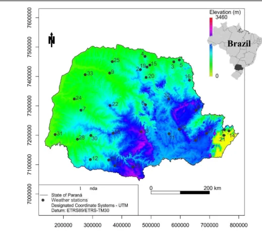
The dataset used in this study is from 33 conventional weather stations of the Agronomic Institute of Paraná (IAPAR) spread across the state (Figure 1 and Table 1). These data represented the period from January 01, 1980 to December 31, 2010, which is a relatively long series of data, thus, there were registration failures of up to 10% of missing data in all studied stations. These failures were fixed with the database developed by Xavier et al. (2015), which interpolates the daily data from various sources and is available in high-resolution spacing (0.25°x0.25°), including all weather variables here evaluated.

Rev. Ambient. Água vol. 12 n. 5 Taubaté – Sep. / Oct. 2017

the reference evapotranspiration (ET0) was carried out through the Penman-Monteith method,

as shown in Equation 1.

ET0=0.408 Δ (Rn − G) + γ [900 / (T + 273)] U_{Δ + γ (1 + 0.34U} 2(ea − es) 2)

(1)

where:

Rn is the net radiation (MJ m-2 _day-1_);

T is the mean temperature of the day, measured at two meters high (°C); U2 is the average wind speed at two meters high (m s-1);

Δ is the slope of the saturated vapor curve (kPa °C-1_);

G is the heat flow of the soil (MJ m-2 _day-1_); γ is the psychrometric constant (kPa °C-1_);

ea is the current vapor pressure (kPa); and

es is the saturation vapor pressure (kPa).

The net radiation was determined by Equation 2, proposed by Allen et al. (1998).

Rn = Qg(1−α) − [4,903 ∙ 10-9 [

Tmax4 + Tmin4

2 ] (0.34 − 0.14 √ea) (1.35 Q_g

Q_gcs − 0.35)] (2) where:

α is the albedo, which was considered as 0.25;

Tmax and Tmin are the maximum and minimum daily temperatures;

Qg is the global solar radiation (MJ m-2 day-1), and

Qcs is the hypothetical solar radiation on a clear-sky day (MJ m-2 day-1), which was

determined by Equation 3. Q_gcs= (0.75 + 2 ∙ 10-5 _{z) Q}

o (3)

where:

z is the local altitude (m), and

Qo is the extraterrestrial radiation (MJ m-2 day-1), based on the latitude of the area and time

of the year, based on the expressions described by Allen et al. (1998).

The ET0 values accumulated were divided into periods of one year (ET0AC). These values

Rev. Ambient. Água vol. 12 n. 5 Taubaté – Sep. / Oct. 2017 Figure 1. Altitude, localization and distribution of weather

stations studied in the state of Paraná, Brazil.

Table 1. Localization and altitude of the weather stations studied the state of Parana, Brazil.

Weather Station Lat. Long. Alt. (m) Weather Station Lat. Long. Alt. (m) 1-Antonina -25.13 -48.48 60 18-Laranjeiras do Sul -25,25 -52.25 880

2-Apucarana -23.30 -51.32 746 19-Londrina -23.22 -51.10 585

3-Bandeirantes -23.06 -50.21 440 20-Mauá da Serra -23.54 -51.13 1020 4-Bela Vista do Paraíso -22.57 -51.12 600 21-Morretes -25.30 -48.49 59

5-Cambará -23.00 -50.02 450 22-Nova Cantu -24.40 -52.34 540

6-Cândido de Abreu -24.38 -51.15 645 23-Palmas -26.29 -51.59 1100

7-Cascavel -24.53 -53.33 660 24-Palotina -24.18 -53.55 310

8-Cerro Azul -24.49 -49.15 360 25-Paranavaí -23.05 -52.26 480

9-Cianorte -23.40 -52.35 530 26-Pato Branco -26.07 -52.41 700

10-Clevelândia -26.25 -52.21 930 27-Pinhais -25.25 -49.08 930

11-Fernandes Pinheiro -25.27 -50.35 893 28-Planalto -25.42 -53.47 400 12-Francisco Beltrão -26.05 -53.04 650 29-Ponta Grossa -25.13 -50.01 880 13-Guarapuava -25.21 -51.30 1058 30-Quedas do Iguaçu -25.31 -53.01 513 14-Guaraqueçaba -25.16 -48.32 40 31-São Miguel Iguaçu -25.26 -54.22 260 15-Ibiporã -23.16 -51.01 484 32-Telêmaco Borba -24.20 -50.37 768 16-Joaquim Távora -23.30 -49.57 512 33-Umuarama -23.44 -53.17 480

17-Lapa -25.47 -49.46 910

Lat. – Latitude; Long. – Longitude; Alt – Altitude.

Rev. Ambient. Água vol. 12 n. 5 Taubaté – Sep. / Oct. 2017 2.3. Trend tests

The trend analysis aimed to identify the maintenance, increase or reduction of the ET0AC

values in the time series, using the non-parametric Mann-Kendall (MK) test.

The MK test was analyzed from the coefficients τ (tau) and s of Mann-Kendall, both used

to identify correlations between the variables. The coefficient τ is defined by the relationship between the score of a real classification of correlation to the maximum possible score. To obtain the score for a data series, the data set should be sorted in ascending order, according to the order of occurrence (chronological), and then the following equation is applied (Equation 4):

S = ∑ ∑sgn(xi−xj) i=n

i=j+1 j=n−1

j=1

(4)

where:

S is the classification score (also called Mann-Kendall sum); x is the value of the data;

i and j are the estimated values of the data sequence; n is the number of data of the series and

sgn is a function that establishes values of -1, 0 and 1, when (x - xj) is negative, zero or positive, respectively.

According to Equation 5, the maximum value of S is:

Smax = 1₂n (n−1) (5)

Thus, Kendall tau (τ) is calculated as (Equation 6). τ = _SS

max (6)

A positive value of s or τ indicates an upward trend, and a negative value indicates a downward trend. However, the probability associated with s or τ and sample size (n) must be calculated to quantify the statistical significance of the trend. Kendall and Gibbons (1990) introduced a normal approach test that can be applied to datasets of more than ten values, with variance s (σ2_{) (Equations 7 and 8).}

σ2 ₌ 1

18 n (n−1)(2n + 5) − CFR (7)

CFR = ₁₈1 ∑mk (mk−1) g

k=1

(2mk + 5) (8)

where:

CFR is a correction factor for repetition, to correct the effect of data groups (when some of

the data values appear more than once in the dataset, this set of values is called linked group); g is the number of linked groups;

Rev. Ambient. Água vol. 12 n. 5 Taubaté – Sep. / Oct. 2017 Then, the normal distribution parameter (called statistics of Mann-Kendall, Z) was calculated by Equation 9.

Z=

{ 1

σ(s−1) se S > 0

0 se S = 0 1

σ (s + 1) se S < 0

(9)

The last step was to find the minimum level of probability in which the Z parameter is significant, using statistical tables (two-tailed) or according to the equation (Equation 10) described by Abramowitz and Stegun (1972).

αmin = (b0 e−0.5Z2) ∑bq q=5

q=1

∙ (1 + b6 ABS(Z))-q (10)

where:

αmin is the minimum level of significance;

q is the number of values;

bx are the constants (b0 = 0.3989,

b1 = 0.3194,

b2 = -0.3566,

b3 = 1.7814,

b4 = -1.8213,

b5 = 1.3303,

b6 = 0.2316); and

ABS(Z) is a function for the absolute value of Z.

The Kendall's tau (τ) is significant at significance level of 5% (p<0.05) when αmin is lower

than a specified value alpha.

The slope of the trend of the data series was calculated according to the method described by Sen (1968). The Sen test must be carried out observing various rules and conditions, such as time series equally spaced, i.e., equal intervals between the data points. However, missing data can be considered in this method. The data must be sorted in ascending order according to the time and then applying (chronological) Equation 11 to calculate the Sen slope estimator (Q) as the median of members of the array of Sen.

Q = Median {[[x₁1−₋x_jj]j=n_j=1−1]_i=j+1i=n } (11)

Rev. Ambient. Água vol. 12 n. 5 Taubaté – Sep. / Oct. 2017

level, i.e. for a 95% confidence level, Z must be evaluated at 0.975, therefore, Z = 1.96. After that, the Cα parameter was calculated from Equation 12.

C_α = Z1-α/2√σ2 (12)

2.4. Geostatistics

With the annual mean values of the variables air temperature, vapor pressure deficit, precipitation and accumulated ET0, a geostatistical analysis of these variables was carried out,

aiming to regionalize them to the study area. The variables were analyzed under the geostatistical models approach (Diggle and Ribeiro Junior, 2007). In this way, the parameters of the model were adjusted by the maximum likelihood method. Different trend models were tested, defined by linear and quadratic relations between the covariates X, Y and elevation at the locations of the meteorological stations. Therefore, the best spatial trend withdrawal model was chosen, and five models of candidate covariance functions were tested: exponential; Gaussian; spherical; circular and matern, with a softness parameter of 1.5 and 2.5. After choosing the model and estimating its parameters, ordinary kriging was used to interpolate the studied variables. The choice of the best model was based on the Akaike Information Criterion (AIC), so the tested distributions that presented the best performance (lower AIC value) were used. The Gaussian model was used to estimate the mean annual temperature. For the variables of vapor pressure, precipitation and ET0, the exponential model was used.

2.5. Data analysis

The precipitation data, estimates of the ET0 series, goodness of fit test and other statistical

calculations were performed using the software XLSTAT-2011.3.02. The software R Statistical 3.1.2® _{(R CORE TEAM, 2016) was used for the geostatistical (geoR, MASS, rgdal and raster}

packages) and graphical (RcolorBrewer, maptools and SDMTools packages) analysis.

3. RESULTS AND DISCUSSION

3.1. Regionalization of the ET0 in the State of Paraná

The spatial distribution of the annual reference evapotranspiration (average of 31 years) (Figure 2A) denotes the combined effect of all the climatological factors that determine this variable.

The average values of ET0AC varied from 578.6 to 1231.9 mm yr-1, denoting a high spatial

variability. The lowest ET0AC was found in Guarapuava, which is located in the south-central

region of the state, at an altitude over 1000 meters, probably due to this region’s milder temperatures. The group with the lowest ET0AC also includes Morretes, Antonina and Pinhais.

The lower ET0AC values were related to high altitudes or proximity to the coast of the regions,

where the maritime is most pronounced (Figure 1 and Table 1).

The region with the highest evapotranspirometric demand is located in the northern portion of the state (Bandeirantes, Paranavaí, Umuarama and Ibiporã), with ET0AC values of about

1200 mm yr-1_{. The counties that integrate this region have highest air temperatures and vapor}

pressure deficit and smaller rainfall accumulated (Figures 2B, 2C and 2D); these conditions justify the magnitude of evapotranspiration in these regions.

Rev. Ambient. Água vol. 12 n. 5 Taubaté – Sep. / Oct. 2017 Figure 2. Spatial variability of the variables: reference evapotranspiration, mm yr-1 (2A); average annual temperature, ºC (2B); average annual vapor pressure deficit, kPa (2C) and accumulated annual rainfall, mm (2D) in the state of Paraná (annual average obtained from the period 1980 -2010).

3.2. ET0 trend analysis in Paraná

The annual and daily mean values of ET0 of each location and the statistical results of the

Mann-Kendall and Sen tests for temporal trend analysis of this variable (Table 2) showed that only 4 of the 33 locations showed significant upward trend (p<0.05) of ET0 values. These

locations were in the eastern (Antonina, Pinhais), south (Cascavel) and north-central (Mauá da Serra) regions of the state. The ET0AC increase rates (Sen test) ranged from 2.53 (Pinhais) to

7.02 mm yr-1 _{(Mauá da Serra).}

The factors affecting the ET0 upward trend for these locations are not clear, mainly due to

the different characteristics of these regions, such as altitude, industrialization level, continentality and maritime. However, Tabari and Talaee (2001a) studied air temperature trends in western Iran and reported increases in the minimum temperature values as the probable cause of increase in evapotranspiration. In fact, significant increases of minimum temperature were found in Cascavel (p-value = 0.03), Mauá da Serra (p-value = 0.01) and Pinhais (p-value = 0.01).

Overall, 70% of the locations studied presented an ET0 upward trend (positive). This result

indicates that the climate variability is affecting the state of Paraná, increasing its

2A 2B

Rev. Ambient. Água vol. 12 n. 5 Taubaté – Sep. / Oct. 2017

evapotranspiration demand with time; however, the analysis of larger historical data is necessary to statistically confirm this trend.

Cambará, Francisco Beltrão, Guaraqueçaba, Ibiporã, Lapa, Morretes, Nova Cantu, Paranavaí, Ponta Grossa and Umuarama presented an ET0 downward trend, although none of

them had statistically significant (p<0.05) tau coefficient (τ). The ET0 analyzes by the Sen

coefficient presented weaker downward trends compared with upward trends, with reduction rates lower than 2.0 mm yr-1_.

ET0 downward trends found in China (Thomas, 2000), Iran (Tabari, et al., 2011b) and India

(Jhajharia et al., 2012) had similar results to those in the present work. According to these authors, the ET0 reductions were due to significant decreases in wind speed and net radiation,

the latter probably due to monsoons, which are common in those regions. Brazil has virtually no monsoons, thus, the reduction of the ET0 can be attributed to the reduction in wind speed,

which, according to Fan and Thomas (2013), is due to changes in the soil surface, thus related to changes of soil coverage and land use and purpose.

Ten locations presented downward ET0 trends, but only three had no significant (p<0.05)

downward trends for wind speed, Ponta Grossa (p=0.5), Francisco Beltrão (p=0.13) and Lapa (p=0.07). These results confirm those found by McVicar et al. (2012), who analyzed 148 studies on wind dynamic around the world and reported that reductions in wind speed have reduced the atmospheric evaporative demand.

The different evapotranspiration demand trends of the State of Paraná were compared and presented positive, negative and neutral variation rates of ET0AC, respectively in Mauá da Serra

(7.0 mm yr-1_{), Paranavaí (-2.0 mm yr}-1_{) and Cerro Azul (0.1 mm yr}-1_{) (Figure 3). Thus,}

according to these results, e.g., variations of trends, the ET0 must be regionalized as a routine

practice in researches related to water demand of terrestrial ecosystems, especially for agriculture due to the importance of water to crop growth.

Figure 3. Trend for evapotranspiration accumulated reference in the locations of Mauá da Serra, Paranavaí and Cerro Azul for the period 1980-2010 in the state of Paraná.

400 500 600 700 800 900 1000 1100 1200 1300 1400

1980 1985 1990 1995 2000 2005 2010

ET

0A

C

C

UM

UL

L

A

T

E

D

(m

m

y

r

-1)

Paranavaí Mauá Cerro Azul

decreasing trend

Rev. Ambient. Água vol. 12 n. 5 Taubaté – Sep. / Oct. 2017 Table 2. Average annual cumulative evapotranspiration (ET0AC), average daily evapotranspiration (ET0D), average rainfall and statistical coefficients of the Mann-Kendall and Sen test for the state of Paraná in the period 1980-2010.

Locality

Reference evapotranspiration Rainfall

ET0AC ET0D CV K-M (τ) Sen’s Slope Average rainfall CV K-M (τ) Sen’s Slope

mm yr-1 _{mm day}-1 _{% Trend mm yr}-1 _{mm yr}-1 _{% Trend mm yr}-1

Antonina 659.3 1.8 12.8 0.3* _{3.2 2315.8 23.9 -0.3}* _-39.5

Apucarana 1062.3 2.9 6.6 0.3ns _{3.3 1619.1 16.6 -0.2}ns _-7.6

Bandeirantes 1231.9 3.4 6.8 0.2ns _{3.3 1442.3 17.5 -0.2}ns _-9.3

Bela Vista 979.0 2.7 5.4 0.0ns _{0.7 1527.1 16.9 -0.4}* _-18.3

Cambará 1139.7 3.1 6.0 0.0ns _{-0.4 1407.7 15.8 -0.2}ns _-5.8

Cândido Abreu 927.9 2.5 7.2 0.18ns _{1.5 1659.3 17.5 -0.2}ns _-7.6

Cascavel 1096.4 3.0 7.4 0.3* _{4.1 1899.9 19.1 -0.4}* _-18.3

Cerro Azul 783.2 2.1 7.7 0.0ns _{0.1 1475.2 18.5 0.3}* _13.0

Cianorte 1120.4 3.1 6.0 0.1ns _{0.8 1627.1 17.5 -0.2}ns _-8.6

Clevelândia 937.87 2.6 6.6 0.1ns _{0.4 2060.0 21.5 0.1}ns _4.4

Fernandes Pinheiro 703.43 1.9 7.2 0.1ns _{1.0 1635.9 20.0 -0.1}ns _-6.0

Francisco Beltrão 905.9 2.5 6.1 -0.2ns _{-1.6 2067.8 22.9 0.0}ns _-3.9

Guarapuava 845.2 2.3 7.0 0.2ns _{1.8 1949.4 18.1 -0.2}ns _-10.3

Guaraqueçaba 578.6 1.6 7.9 -0.1ns _{-1.0 2452.7 16.1 0.1}ns _7.7

Ibiporã 1164.1 3.2 7.1 -0.1ns _{-1.5 1515.3 18.6 -0.1}ns _-8.0

Joaquim Távora 1057.8 2.9 5.6 0.0ns _{0.4 1432.8 15.0 -0.1}ns _-2.2

Lapa 715.9 2.0 6.4 -0.1ns _{-1.1 1548.8 18.6 0.1}ns _6.9

Laranjeiras do Sul 913.9 2.5 7.3 0.2ns _{2.5 2055.5 17.3 -0.1}ns _-8.9

Londrina 1102.8 3.0 6.6 0.0ns _{0.9 1619.6 18.1 -0.1}ns _-3.6

Mauá da Serra 967.2 2.7 10.5 0.4* _{7.0 1642.4 19.9 -0.4}* _-17.9

Morretes 597.0 1.6 7.6 -0.2ns _{-1.7 2018.2 15.5 0.1}ns _7.4

Nova Cantu 1069.1 2.9 6.7 -0.1ns _{-1.3 1988.6 14.3 -0.1}ns _-8.9

Palmas 768.54 2.1 6.3 0.1ns _{0.6 2110.0 20.4 0.0}ns _0.9

Palotina 1041.7 2.9 6.0 0.1ns _{0.7 1662.2 21.2 -0.0}ns _-3.2

Paranavaí 1187.8 3.3 6.9 -0.2ns _{-2.0 1487.3 16.8 0.0}ns _-1.2

Pato Branco 925.64 2.5 5.9 0.1ns _{0.8 2072.4 23.4 -0.1}ns _-5.2

Pinhais 667.7 1.8 11.7 0.3* _{2.5 1503.0 17.2 0.0}ns _3.6

Planalto 1066.9 2.9 6.1 0.0ns _{0.7 1968.0 20.4 -0.1}ns _-5.1

Ponta Grossa 839.4 2.3 6.4 -0.2ns _{-2.0 1624.5 20.7 0.0}ns _0.3

Quedas do Iguaçu 966.0 2.6 7.0 0.2ns _{2.8 1994.1 18.6 -0.2}ns _-11.6

São Miguel Iguaçu 1031.4 2.8 5.8 0.2ns _{2.3 1820.5 16.9 -0.2}ns _-7.6

Telêmaco Borba 814.6 2.2 5.7 0.1ns _{1.3 1622.8 14.9 -0.1}ns _-6.4

Umuarama 1180.5 3.2 6.6 -0.1ns _{-1.4 1630.9 15.6 0.0}ns _-0.5

ET0AC– Evapotranspiration accumulated reference; ET0D– Evapotranspiration daily reference; CV – Coefficient of Variation; M-K – Mann-Kendall’s test; Sen’s Slope –

Rev. Ambient. Água vol. 12 n. 5 Taubaté – Sep. / Oct. 2017 3.3. Regionalization of the precipitation in Paraná

The spatial variability of the precipitation in the State of Paraná from 1980 to 2010 ranged from 1407.7 mm yr-1 _{in Cambará (northeast) to 2452.6 mm yr}-1 _{in Guaraqueçaba (north coast)}

(Figure 2D).

The highest precipitation occurred, in general, in the coastal and south-central regions of the state, with precipitation amounts above 2000 mm yr-1_{. According to the Koppen}

classification, these regions have climate type Cfb, which is characterized by the occurrence of abundant and well-distributed rainfall throughout the year. These characteristics may be related to the high altitudes of these regions (Figure 1), which slow air masses and frontal systems that promote rains from the coast (Nascimento Jr. and Sant'Anna Neto, 2015).

The regions with the lowest precipitations were the northwest and northeast, with precipitation amounts lower than 1500 mm yr-1_{; however, Paraná has a low risk of soil water}

deficit, although this possibility must be assumed for some annual crops, mainly for those with socio-economic importance in these regions. The central region presented a significant and differentiated precipitation variability compared with the northwest, north, east and northeast regions of the state, with depths of about 1800 mm yr-1_.

The Paraná municipalities had high precipitation variability within the year, with amounts ranging from 800 to 3400 mm yr-1 _{(Figure 4).}

Figure 4. Bloxplot of the variability of annual accumulated rainfall, in the period 1980-2010, for the 33 studied municipal districts.

According to Sousa and Nery (2002) the phenomenon El Niño Southern Oscillation (ENSO), which presents anomalies of atmospheric pressure and temperature in the surface of the Equatorial Pacific Ocean, classified as El Niño (positive phase) and La Niña (negative

Av

e

ra

ge

a

n

n

u

al

ra

in

fal

l

(m

m

y

r

-1) 0

500 1000 1500 2000 2500 3000 3500

Rev. Ambient. Água vol. 12 n. 5 Taubaté – Sep. / Oct. 2017 phase), is one of the main large-scale factors that contribute to changes in atmospheric circulation, which are responsible for the precipitation variability within the year. Effects related to maritime (Atlantic Ocean), continentality (central and western state), relief (southern Geral Sierra and eastern Sea Sierra) and latitude (Tropic of Capricorn in the north) affect the precipitation to a lesser extent (regional level). Thus, to understand how these factors affect the precipitation dynamics of the state is important to identify their effect on activities that are dependent on them.

3.4. Precipitation trend analysis in Paraná

The average values of annual precipitation of each municipality and the statistical results of the Mann-Kendall and Sen tests for temporal trend analysis of this variable (Table 2), similarly to the results for the evapotranspiration, presented significant (p<0.05) trends in five (Bela Vista do Paraíso, Cerro Azul, Antonina, Cascavel and Mauá da Serra) of the 33 locations studied. However, different from the evapotranspiration, the precipitation trend was downward in these locations, except in Cerro Azul, which presented an upward trend.

The results showed temporal trends (significant at 5%); however, 76% of the locations studied (25 municipalities) showed downward precipitation trends. Among the locations with upward trends, Cerro Azul, located in the east of the state, was the only one that had a significant (p<0.05) upward trend.

The variation rates from the Sen test showed decreasing rainfall of up to 39.5 mm yr-1

(Antonina) and increasing rainfall of up to 13.0 mm (Cerro Azul). The municipalities Palmas, Ponta Grossa and Umuarama had the lowest increasing/decreasing rates of annual precipitation, with amounts lower than 1 mm.

The results found in this study differ from those found by Minuzzi and Caramori (2011), who verified a trend of precipitation increase in the state of Paraná when they analyzed data from 21 hydrological stations. However, more recent research by Silva et al. (2015) corroborate the results identified in this study, since these authors verified trends of reduction in the annual rainfall in Paraná, mainly in the central and northern regions of the Paraná state, with increasing rainfall behavior only in the coast and southwest of the state.

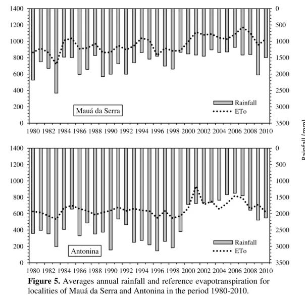
Finally, we verify that the variables evapotranspiration and precipitation did not show statistically significant trends (p <0.05) in most of the stations analyzed in the state of Paraná. For municipalities where significant trends have been identified, these are located in distinct mesoregions of the territory of Paraná, and there is no evidence of specific regional behavior. However, when the analysis is restricted only to these municipalities, it can be observed that the behavior for the two variables is antagonistic, as can be observed in Figure 5, where the municipalities of Mauá da Serra and Antonina show increases in the annual values of evapotranspiration and decreases for accumulated precipitation. As reported by Collischonn and Tucci (2014) in a study that involved monthly relations between these two variables, this behavior is not uncommon, considering that a higher frequency of precipitation events tends to increase the relative humidity of the air, which in turn, would promote a reduction in the evapotranspirometric demand of the atmosphere.

Rev. Ambient. Água vol. 12 n. 5 Taubaté – Sep. / Oct. 2017 Re fe re n ce ev ap o tra n sp irat ion (mm ) Rai n fal l (m m )

4. CONCLUSIONS

The analysis of the evapotranspiration (ET) demand in the State of Paraná indicated that the ET0 increases from the coast to the interior of the state, with the highest values in the

northeast and northwest regions, reaching 1200 mm yr-1_{. The temporal results of the ET showed}

a significant upward trend in 4 of the 33 locations studied, with increases ranging from 2.5 to 7.0 mm yr-1_.

Precipitation presented the highest amounts in the coastal and south-central regions and the lowest amounts in the northeast and northwest regions. The precipitation trend analysis indicated a significant downward trend in the precipitation volume of five locations.

The evapotranspiration and precipitation showed, in general, no statistically significant trends in most of the stations analyzed; however, the upward trends for ET and downward trends for precipitation indicate local changes in the State of Paraná.

5. ACKNOWLEDGEMENTS

We would like to thank the funding agency Coordenação de Aperfeiçoamento de Pessoal

de Nível Superior (CAPES) for the post-doctoral scholarship of the first author and also the

financial support through funding PNPD/CAPES (Agreement UEG/CAPES N. 817164/2015-PROAP). The authors also thank IAPAR and University of São Paulo for the necessary support.

0 500 1000 1500 2000 2500 3000 3500 0 200 400 600 800 1000 1200 1400

1980 1982 1984 1986 1988 1990 1992 1994 1996 1998 2000 2002 2004 2006 2008 2010

Mauá da Serra

Rainfall ETo 0 500 1000 1500 2000 2500 3000 3500 0 200 400 600 800 1000 1200 1400

1980 1982 1984 1986 1988 1990 1992 1994 1996 1998 2000 2002 2004 2006 2008 2010

Antonina

Rainfall ETo

Rev. Ambient. Água vol. 12 n. 5 Taubaté – Sep. / Oct. 2017

6. REFERENCES

ABRAMOWITZ, M.; STEGUN, I. A. Handbook of Mathematical Functions with Formulas. Graphs. and Mathematical Tables. 10. ed. New York: Wiley, 1972. 1046 p.

ALLEN, R. G.; PEREIRA, L. S.; RAES, D.; SMITH, M. Crop evapotranspiration: guidelines for computing crop water requirements. Rome: FAO, 1998. 297p. (Irrigation and drainage paper, 56).

COLLISCHONN, B.; TUCCI, C. E. M. Relações regionais entre precipitação e evapotranspiração mensais. Revista Brasileira de Recursos Hídricos, v. 19, p. 205-214, 2014.

COMPANHIA NACIONAL DE ABASTECIMENTO – CONAB. Séries históricas de área plantada, produtividade e produção, relativas às safras 1976/77 a 2015/16 de grãos. 2001 a 2016 de café. 2005/06 a 2016/17 de cana de açúcar. 2016. Available in: http://www.conab.gov.br/conteudos.php?a=1252&t=. Access in: September 2016. DIGGLE, P. J.; RIBEIRO JÚNIOR, P. J. Model-based geostatistics. Londres: Springer, 2007.

230p.

FAN, Z.; THOMAS, A. Spatiotemporal variability of reference evapotranspiration and its contributing climatic factors in Yunman Province. SW China. 1961-2004. Climate Change, v. 116, n. 2, p. 309-325, 2013. http://dx.doi:10.1007/s10584-012-0479-4 HESS, T.; DACCACHE, A.; DANESHKHAH, A.; KNOX, J. Scale impacts on spatial

variability in reference evapotranspiration. Hydrological Science Journal, v. 61, n. 3, p. 601-609, 2016. http://dx.doi.org/10.1080/02626667.2015.1083105.

JERSZURKI, D.; SOUZA, J. L. M.; EVANGELISTA, A. W. P. Probabilidade e variação temporal da evapotranspiração de referência na região de Telêmaco Borba – PR. Revista Brasileira de Biometria, v. 33, n. 2, p. 118-129, 2015.

JHAJHARIA, D.; DINPASHOH, Y.; KAHYA, E.; SINGH, V. P.; FAKHERI-FARD, A. Trends in reference evapotranspiration in the humid region of northeast India. Hydrological Processes, v. 26, n. 3, p. 421-435, 2012. http://dx.doi:10.1002/hyp.8140 KENDALL, M.; GIBBONS, J. D. Rank Correlation Methods. 5. ed. New York: A Charles

Griffin Book, 1990. 272p.

KHALIL, A. A.; ESSA, Y. H.; ABDEL-WAHAB, M. M. Evapotranspiration mapping over Egypt using MODIS/Terra satellite data. International Journal of Advanced Research, v. 15, n. 12, p. 512-522, 2015.

LI, Z. L.; TANG, R.; WAN, Z.; BY, Y.; ZHOU, C.; TANG, B.; YAN, G.; ZHANG, X. A review of current methodologies for regional evapotranspiration estimation from remotely sensed data. Sensor, v. 9, p. 3801-3853, 2009. http://dx.doi.org/10.3390/s90503801.

Rev. Ambient. Água vol. 12 n. 5 Taubaté – Sep. / Oct. 2017

McVICAR, T. R. et al. Global review and synthesis of trends in observed terrestrial near-surface wind speeds: Implications for evaporation. Journal of Hydrology, v. 416-417, p. 182-205, 2012. http://dx.doi.org/10.1016/j.jhydrol.2011.10.024

MINUZZI, R. B.; CARAMORI, P. H.; Variabilidade climática sazonal e anual da chuva e veranicos no estado do Paraná. Revista Ceres, v. 58, n. 5, p. 593-602. 2011,

http://dx.doi.org/10.1590/S0034-737X2011000500009

NASCIMENTO JÚNIOR, L.; SANT’ANNA NETO, J. L. Contribuição aos estudos da precipitação no estado do Paraná: a oscilação decadal do pacífico – ODP. Revista Raega, v. 35, p. 314-343, 2015. http://dx.doi.org/10.5380/raega.v35i0.42048

PEDRON, I. T.; KLOSOWSKI, E. S. Distribuição de frequência de chuvas diárias no Estado do Paraná. Scientia Agraria Paranaensis, v. 7, n. 1-2, p. 55-63, 2008. http://dx.doi.org/10.1818/sap.v0i0.2052

R CORE TEAM. R: A language and environment for statistical computing. R Foundation for Statistical Computing. Vienna, 2016. Available in: https://www.R-project.org/. Access in: September 2016.

SEN, P. K. Estimates of the regression coefficient based on Kendall’s TAU. Journal of the American Statistical Association, v. 63, p. 1379-1389, 1968. http://dx.doi.org/10.2307/2285891

SENTELHAS, P. C.; GILLESPIE, T. J.; SANTOS, E. A. Evaluation of FAO Penman–Monteith and alternative methods for estimating reference evapotranspiration with missing data in Southern Ontario. Canada. Agricultural Water Management, v. 97, n. 5, p. 635-644, 2010. http://dx.doi.org/10.1016/j.agwat.2009.12.001

SILVA, M. E. S.; GUETTER, A. K. Mudanças climáticas regionais observadas no estado do Paraná. Revista Terra Livre, v. 1, n. 20, p. 111-126, 2003.

SILVA, W. L.; DERECZYNSKY, C.; CHANG, M.; FREITAS, M.; MACHADO, B. J.; TRISTÃO, L.; RUGGERI, J. Tendências observadas em indicadores de extremos climáticos de temperatura e precipitação no estado do Paraná. Revista Brasileira de Meteorologia, v. 30, n. 2, p. 181-194, 2015. http://dx.doi.org/10.1590/0102-778620130622

SOUZA, J. L. M.; JERSZURKI, D.; GOMES, S. Precipitação e evapotranspiração de referência prováveis na região de Ponta Grossa – PR. Irriga, v. 19, n. 2, p. 279-291, 2014. http://dx.doi.org/10.15809/irriga.2014v19n2p279.

SOUSA, P.; NERY, J. T. Análise da variabilidade anual e interanual da precipitação pluviométrica da região de Manuel Ribas. Estado do Paraná. Acta Scientiarum, v. 24, n. 6, p. 1707-1713, 2002. http://dx.doi.org/10.4025/actascitechnol.v24i0.2513

TABARI, H.; TALAEE, P. H. Recent trends of mean maximum and minimum air temperatures in the western half of Iran. Meteorology and Atmospheric Physics, v. 111, n. 3, p. 121-131, 2011a. http://dx.doi:10.1007/s00703-011-0125-0

Rev. Ambient. Água vol. 12 n. 5 Taubaté – Sep. / Oct. 2017 THOMAS, A. Spatial and temporal characteristics of potential evapotranspiration trends over

China. International Journal of Climatology, v. 20, p. 381-396, 2000. http://dx.doi:10.1002/(SICI)1097-0088(20000330)20:4<381::AID-JOC477>3.0.CO;2-K XAVIER, A. C.; KING, C. W.; SCANLON, B. R. Daily gridded meteorological variables in

Brazil (1980-2013). International Journal of Climatology, v. 36, n. 6, p. 2644-2659, 2015. http://dx.doi:10.1002/joc.4518