Dynamic modelling of a 3-CPU parallel robot via screw theory

www.mech-sci.net/4/185/2013/ doi:10.5194/ms-4-185-2013

©Author(s) 2013. CC Attribution 3.0 License.

Mechanical

Sciences

Open Access

Dynamic modelling of a 3-CPU parallel

robot via screw theory

L. Carbonari, M. Battistelli, M. Callegari, and M.-C. Palpacelli

Universit`a Politecnica delle Marche, Via Brecce Bianche, 60131, Ancona, Italy

Correspondence to: L. Carbonari ([email protected])

Received: 15 November 2012 – Revised: 15 March 2013 – Accepted: 5 April 2013 – Published: 24 April 2013

Abstract. The article describes the dynamic modelling of I.Ca.Ro., a novel Cartesian parallel robot recently designed and prototyped by the robotics research group of the Polytechnic University of Marche. By means of screw theory and virtual work principle, a computationally efficient model has been built, with the final aim of realising advanced model based controllers. Then a dynamic analysis has been performed in order to point out possible model simplifications that could lead to a more efficient run time implementation.

1 Introduction

Many approaches are available for the dynamic modelling of multi-body mechanical systems (Kovecses et al., 2003; Moon, 2008; Papastavridis, 2012) and in the last years, many most of them have been investigated by robotics researchers to achieve efficient models of robots dynamics. Indeed, the efficiency in computation of inverse dynamics of robotic ma-nipulators has a fundamental importance if such tools are in-volved in the implementation of model based control algo-rithms whose effectiveness is strongly affected by the compu-tational efficiency of the mathematical model (Lin and Song, 1990; Wang et al., 2007). Thus, it is interesting to investi-gate the possibility to build simplified dynamics models, es-pecially for parallel kinematic machines that are character-ized by an inherent toughness due to the closed kinematic structure. Such peculiarity often complicates the computa-tion of the dynamic model and sometimes prevents the use of model based controls. This inherent complexity is the main reason why only few dynamic models of parallel robots are presently available in scientific literature in symbolic form (Dasgupta and Mruthyunjaya, 1998; Tsai, 2000; Caccavale et al., 2003).

The traditional Newton-Euler formulation, which has been widely used in the past (Do and Yang, 1988; Dasgupta and Mruthyunjaya, 1998) and is still used for specific tasks by some researchers (Kunquan and Rui, 2011; Khalil and Ibrahim, 2007), hardly adapts to the particular case of par-allel kinematics machines.

As a matter of fact, all mechanical principles have been used to carry on dynamic analysis of robotic systems, such as the generalized momentum approach (Lopes, 2009), the Hamilton’s principle (Miller, 2004), the Lagrange formula-tion (Wronka and Dunnigan, 2011; Di Gregorio and Parenti-Castelli, 2004) and the virtual work principle (Zhang and Song, 1993).

In order to formulate the dynamic model of a mechanical system, the knowledge of its position kinematics is strictly necessary. As a matter of fact, the solution of the forward kinematics problem (FKP) of a parallel platform represents a challenging issue that not necessarily yields to a closed form solution, especially when the robot end-effector is allowed to perform motions of rotation.

As argued by authors in past works (Carbonari, 2012; Car-bonari and Callegari, 2012) the 3-CPU parallel architecture can provide the end-effector with different kinds of mobility, depending on the mutual configuration of the joints that com-pose the leg’s kinematic chain. Carbonari et al. (2013) also demonstrated that a reconfiguration of the universal joint al-lows to modify the kinematic behaviour of a 3-CPU parallel robot, switching from a pure rotational to a pure translational kinematic behaviour.

This paper focuses on the dynamic modelling of a pure translational 3-CPU architecture, called I.Ca.Ro. by Calle-gari and Palpacelli (2008), aimed at the realization of a non-linear model based control scheme. The main object of the present work is to produce a numerically efficient dynamic model of the machine, suitable to be used for the realization of a control algorithm. To this aim, the differential kinemat-ics of the manipulator has been tackled taking advantage of a screw based approach (Gallardo et al., 2003). For the seek of completeness, the position kinematics is also presented here in order to improve the reader’s understanding of the prob-lem.

2 Robot kinematics

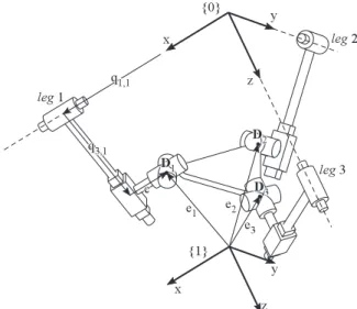
The I.Ca.Ro. parallel robot is a pure translational Carte-sian tripod whose limbs are built of a C-P-U (cylindrical-prismatic-universal) joints chain. The first body of each leg is connected to the robot chassis by means of a cylindrical joint, realized through a prismatic actuated pair and a rev-olute passive joint coaxial to the first one (refer to Fig. 1). The second body is linked to the first one through a pris-matic joint, perpendicular to the axis of the cylindrical joint. At last, the second body is connected to the moving platform through a universal joint composed of two revolutes: the first revolute joint is parallel to the second link and the second is perpendicular to the first one. The last revolute of each leg connects the manipulator with the respective limb; the axes of such joints are coplanar.

Due to the robot kinematic architecture, the I.Ca.Ro. par-allel manipulator is only able to provide the end-effector with pure translations. In fact, by means of screw theory it can be observed that each leg exerts a constraint wrench made of a pure torque along the direction of its passive prismatic pair. The connection of the three legs to the mobile platform pro-duces a wrench system of three orthogonal torques, whose dual space is spanned by a basis of three linearly independent pure translations. Thus, the orientation of a reference frame

Figure 1. Kinematics of the 3-CPU pure translational parallel robot.

that solidly moves with it remains constant notwithstanding the displacement that the actuated joints perform.

With respect to the notation introduced in Fig. 1, the ho-mogeneous transformation matrix that describes the configu-ration of reference frame_{1_}with respect to reference frame {0_}can be expressed as:

0_T 1=

             

1 0 0 px

0 1 0 py

0 0 1 pz

0 0 0 1

             

(1)

where px, py and pz denote the position of the centre of the moving frame_{1_} and the 3 by 3 identity rotation ma-trix suggests that the orientation of the manipulator remains constant.

The forward and inverse kinematics problems of the robot can be easily solved taking advantage of three loop clo-sure equations. The positions of the three attachment points Di between the end-effector and the three limbs can be simply reached through the transformation matrix0_T

1,

be-ing their position fixed with respect to reference frame_{1_}:

Di=0T1

h

eT

i 1

iT

, where e1=−e

h

0 1/√2 1/√2iT, e2=

−eh1/√2 0 1/√2iT, e3=−e

h

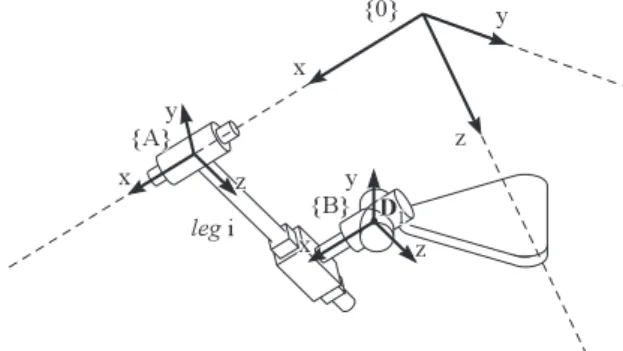
1/√2 1/√2 0iT. As it is shown in the following, the coordinates of such points can be also reached through the use of legs’ joints displace-ments. The comparison between the different expressions of these three points provides the solution of the problem. The reference frames shown in Fig. 2 are used to define legs kine-matics.

Figure 2.Reference frames along leg structure. like: 0_T A=              

1 0 0 q1,1

0 cq2,1 −sq2,1 0

0 sq2,1 cq2,1 0

0 0 0 1

              (2)

where q2,1 denotes the rotation of the cylindrical pair of the

leg 1 and shorthand notation is used for trigonometric func-tions. To reach the configuration of the third reference frame {B_}, thus the position of attachment point D1, a translational

transformation matrix is sufficient:

A_T B=              

1 0 0 ₋c

0 1 0 0

0 0 1 q3,1

0 0 0 1

              (3)

with q3,1 denoting the displacement performed by prismatic

pair of the first leg. Coordinates of point D1 can now be

achieved as:

D1=0TAATB

h

0 0 0 1iT (4)

Since the kinematic chain is identical for each leg, it is not necessary to explicit their homogeneous transformations as specific cases. Indeed, Eq. (4) can be exploited if pre multi-plied by a transformation that rotates the starting reference frame. In particular, it is possible to define the matrices:

0_T leg2=              

0 0 1 0

1 0 0 0

0 1 0 0

0 0 0 1

              0_T leg3=              

0 1 0 0

0 0 1 0

1 0 0 0

0 0 0 1

              (5)

such that the coordinates of the remaining attachment points can be expressed as:

D2=0Tleg2leg2TAATB

h

0 0 0 1iT

D3=0Tleg3leg3TAATB

h

0 0 0 1iT

(6)

Even if it is not specified, it should be evident that transfor-mationsleg2TA,leg3TAandATBof the 2nd and 3rd equations

in (6) are expressed in terms of the respective joints variables

q1,i, q2,iand q3,i.

In order to give a general expression of legs kinematics, it is also introduced the matrix0_T

leg1, an identity 4 by 4 matrix

that allows to write the Eq. (4) as:

D1=0Tleg1leg1TAATB

h

0 0 0 1iT (7)

whereleg1_T

A=0TA.

Expansion of (6) and (7) yields to the expression of such points coordinates in terms of joints variables, that are:

D1=

             

q1,1−c

q3,1sq2,1

−q3,1cq2,1

1              

D2=

             

−q3,2cq2,2

q1,2−c

q3,2sq2,2

1              

D3=

             

q3,3sq2,3

−q3,3cq2,3

q1,3−c

1               (8)

Equations (8) can be inverted to achieve the expression of legs joints variables as functions of coordinates of the three attachment points Di:

q1,1=D1,x+c

q1,2=D2,y+c

q1,3=D3,z+c

q2,1=tan−1 D1 ,y

−D1,z q2,2=tan−1 D_−D2,z

2,x q2,3=tan−1 D3

,x

−D3,y

q3,1=

D1,y

sin q2,1

q3,2=

D2,z

sin q2,2

q3,3=

D3,x

sin q2,3

(9)

It is worth to remark that such coordinates are uniquely de-termined if the pose of the manipulator is known.

3 Velocity kinematics

In order to build the Jacobian matrices of a PKM, both po-sition and orientation of the joints axes are needed. Firstly it is necessary to define an appropriate number of reference frames preferably attached in convenient points of the kine-matic chain. It is worth to remember that the screws must be expressed with respect to a reference frame attached to robot manipulator and whose orientation is constant and coincident to that of robot absolute reference frame_{0_}. Furthermore, in order to define the dynamical model of the machine, the mov-ing frame should be centred at the c.o.m. of the body object of the velocity analysis.

In the case of the pure translational robot I.Ca.Ro. the moving platform reference frame _{1_} represents a feasible choice for expressing the screw coordinates. In fact, it is solid with the end-effector and it does not rotate; moreover, due to the pure translational mobility of the end-effector, the origin of frame_{1_}moves with the same velocity and acceleration of the end-effector c.o.m. even if it is not centred on it.

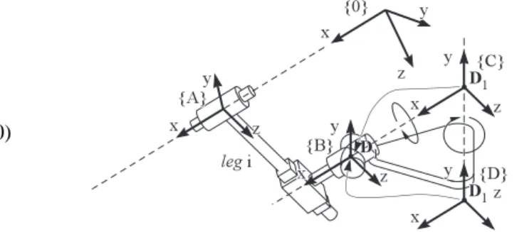
The screw coordinates of every kinematic pair involved in leg kinematic chain must be expressed: to this aim, conve-nient local frames must be arranged along the legs as shown in Fig. 3.

are defined as: B_T C=              

1 0 0 0

0 cq4,1 −sq4,1 0

0 sq4,1 cq4,1 0

0 0 0 1

              C_T D=              

cq5,1 0 sq5,1 0

0 1 0 0

−sq5,1 0 cq5,1 0

0 0 0 1

              (10)

The pose of frames_{A_},_{B_},_{C_}and_{D_}is described by the following homogeneous transformations:

1_T

A,1=1T00Tleg1leg1TA

1_T

B,1=1T00Tleg1leg1TAATB

1_T

C,1=1T00Tleg1leg1TAATBBTC

1_T

D,1=1T00Tleg1leg1TAATBBTCCTD

(11)

The unit vectors of joints’ axes can be easily expressed in the global frame by means of the proper mapping between the local frames and the global one:

– Joint 1, prismatic:

"

s1,i 1

# =1_T

A,i

              1 0 0 1              

→ S1,i=

" 0

s1,i

#

(12)

– Joint 2, revolute:

"

s2,i

1

# =1_T

A,i

               1 0 0 1                "

r2,i

1

# =1_T

A,i

               0 0 0 1               

→S2,i=

"

s2,i

r2,i×s2,i

#

(13)

– Joint 3, prismatic:

"

s3,i 1

# =1TA,i

              0 0 1 1              

→ S3,i

" 0

s3,i

#

(14)

– Joint 4, first revolute of the universal joint:

"

s4,i

1

# =1_T

B,i

               1 0 0 1                "

r4,i

1

# =1_T

B,i

               0 0 0 1               

→S4,i=

"

s4,i

r4,i×s4,i

#

(15)

– Joint 5, second revolute of the universal joint:

"

s5,i

1

# =1_T

C,i

               0 1 0 1                "

r5,i

1

# =1_T

C,i

               0 0 0 1               

→S5,i=

"

s5,i

r5,i×s5,i

#

(16)

Figure 3.Local frames used for definition of joints unit screws.

In order to simplify expressions of manipulator Jacobian ma-trices it is possible to use three screws which have the main characteristic of being reciprocal to all unit screws of the leg, with the exception of the actuated joints screws. Such screws are here called Sr,i.

To this aim, it is possible to make use of the unit screw S4,i shown in Fig. 4, which turns reciprocal to each non-actuated screw present in the leg kinematic chain due to the fact that it is coplanar to both S2,iand S5,i, it intersects the axis of the

prismatic joint described by S3,iand, by definition, it is recip-rocal to itself. Furthermore, it is not reciprecip-rocal to S1,ibeing parallel but not aligned to the axis of the actuated prismatic joint.

At this point vector expressions have been given for joints screws and for legs reciprocal screws. The Jacobian ma-trices can be formulated in order to achieve an expres-sion for the velocity problem which has the well known form JX˙x=JQq, where ˙x is the velocity vector of the˙ platform that, in a general way, can be expressed as ˙x= h

ωx ωy ωz ˙qx ˙qy ˙qz

iT

.

Firstly it is introduced the Jacobian matrix JX, whose ex-pression can be formulated as a function of reciprocal screws:

JX=

          ST

r,1

ST

r,2

ST

r,3           =           ST

4,1

ST

4,2

ST

4,3           =          

0 q3,1cq2,1−pz q3,1sq2,1+py 1 0 0

q3,2sq2,2+pz 0 q3,2cq2,2−px 0 1 0

q3,3cq2,3−py q3,3sq2,3+px 0 0 0 1

          (17)

The moving platform of I.Ca.Ro. PKM is only allowed to perform pure translations; this implies that the first three components of the vector ˙x, i.e. ωx, ωy andωz, are iden-tically null. As a consequence, such components and the first three columns of matrix JX can be eliminated due to the fact that the do not give any contribution to equation

JX˙x=JQq. Thus, the Jacobian J˙ X is a three by three iden-tity matrix which multiplies the end-effector velocity vector

Figure 4.Unit screws of each kinematic joints.

Finally matrix JQis introduced:

JQ=

         

ST_r,1S1,1 0 0

0 ST

r,2S1,2 0

0 0 ST

r,3S1,3

          =          

1 0 0

0 1 0

0 0 1

          (18)

Due to pure translational robot kinematic behaviour, the end-effector velocity problem can be simply expressed as:

         

1 0 0

0 1 0

0 0 1

                    ˙px ˙py ˙pz           =          

1 0 0

0 1 0

0 0 1

                    ˙ d1 ˙ d2 ˙ d3           (19)

Thanks to the screw based approach, the velocities of pas-sive joints have been eliminated from the formulation of end-effector velocity kinematics. Nevertheless this information is needed to perform other types of analysis such as the study of robot dynamics.

Thus, the knowledge of the velocity vectors of each mem-ber composing the legs is necessary and it can be achieved through the computation of passive joints velocity as func-tions of active joints rates. To this aim, robot architecture constraint equations are exploited to build a matrix A relating prismatic actuated joints velocities to all other rates:

˙

qp=A ˙qa (20)

where ˙qpis a vector collecting velocities of passive joints and

˙

qais the vector of actuated joints rates.

The main aim of this computation is to provide the needed tools for the dynamic modelling of the robotic system. There-fore, a simplification based on influence of each body is introduced yielding a relevant computational simplification. The mass of the elements that compose the revolute joints is negligible if compared with masses of legs linkages and translating parts of prismatic actuators. Hence, it is supposed here that they only marginally affect the whole dynamic be-haviour of the robot: thus, their contribution is not consid-ered. This simplification is reasonably acceptable and enor-mously simplifies robot model because of the complexity in-troduced by the velocity expressions of these elements.

Such simplification allows us to reduce the dimension of matrix A. If the actual number of active and passive joints is considered, Eq. (20) can be expanded to:

                        

˙q2,1

˙q2,2

˙q2,3

˙q3,1

˙q3,2

˙q3,3

                         =A          

˙q1,1

˙q1,2

˙q1,3

          (21)

where ˙q1,i is the translation rate of cylindrical pair of i-th leg, ˙q2,i is the rotation rate of the same pair and ˙q3,i is the translation rate of the passive prismatic joint.

The constraint matrix A can be built considering the mo-bility of each attachment point between legs and manipula-tor; indeed, the velocity of such points is known and equal to the velocity of the moving platform due to the fact that they solidly move with the end-effector which only performs pure translational motions. The velocities of passive joints can be related to the components of the velocity vectors as visible in Fig. 5 for a general mobility.

The component of vD,ialong the direction perpendicular to leg plane is expressed by:

v⊥_D,i=vT_D,i s2,i×s3,i (22)

The velocity along this direction is fully due to the rotation of the cylindrical joint, so that:

˙q2,i= vT

D,i s2,i×s3,i

q3,i

(23)

The component of velocity that lies on the leg plane is due to both the actuated and non actuated prismatic joints:

˙q1,i=vT_D,is1,i ˙q3,i=vTD,is3,i

(24)

The first equation in (24) simply relates the velocity along the axis of the cylindrical joint to the actuation rate; thus, it is not useful for the construction of the constraint matrix. On the other hand, the second equation can be used for the scope. Equation (23) and the second equation in (24) can be ex-panded and written in the matrix form (20). In the case of a pure translational robot the velocities of legs attachment points correspond to the velocity of the origin of end effector reference frame. Exploiting Eqs. (22) and the second of (24), expressions of non actuated joints rates are achievable. In this case, the simplification introduced by end-effector mobility allows to show which is the actual shape of such expressions.

For the revolute joints it is:

˙q2,1=−

˙q1,2cq2,1−˙q1,3sq2,1

q3,1

˙q2,2=−

˙q1,1sq2,2−˙q1,3cq2,2

q3,2

˙q2,3=−

˙q1,1cq2,3−˙q1,2sq2,3

q3,3

Figure 5.Velocity of attachment points between legs and moving platform.

while prismatic joints rates are:

˙q3,1 = −˙q1,2sq2,1+˙q1,3cq2,1

˙q3,2 = ˙q1,1cq2,2−˙q1,3sq2,2

˙q3,3 = −˙q1,1sq2,3+˙q1,2cq2,3

(26)

Hence, the matrix formulation of the 6 passive velocities is:

                        

˙q2,1

˙q2,2

˙q2,3

˙q3,1

˙q3,2

˙q3,3

                         =                           

0 −cq2,1

q3,1

−sq2,1

q3,1

−sq2,2

q3,2 0

−cq2,2

q3,2

−cq2,3

q3,3

−sq2,3

q3,3 0

0 ₋sq2,1 cq2,1

cq2,2 0 −sq2,2

−sq2,3 cq2,3 0

                                    

˙q1,1

˙q1,2

˙q1,3

          (27)

In the remainder of this work, the constraint matrix is used to express the velocity of the reference frames attached to the robot bodies. To do that, further Jacobian matrices are introduced. In particular, the velocity of the c.o.m. of each body is written according to the general formulation:

˙x=J ˙qa (28)

where ˙qais the vector of actuated joints rates.

It is important to remark that the target of this section is the definition of legs bodies velocities, whose serial kinemat-ics chain does not allow the simplification of passive joints

rates. Thus, the Jacobian formulation ˙x=˜Jhq˙T

a q˙Tp

iT

in-volves also the velocity of non actuated joints. Nevertheless, the influence of such joints can be explicited by means of the constraint matrix (27). Equation (28) becomes:

˙x=˜J "

I A

# ˙

qa (29)

where I is a 3_×3 identity matrix; the matrices ˜J can be very quickly expressed taking advance of joints screws; thus the

formulation of legs velocities turns out to be an immediate iterative process based on collection of already introduced vectors.

Firstly, the velocities of the three sliders are achieved: for the sake of conciseness, these bodies are denoted as sl1, sl2

and sl3 with reference to the leg which they are part of. The

serial chain that allows reaching their screw is composed only by the actuated prismatic pair. In this case the body is not allowed to rotate, so that the position of the screw axis does not influence the screw expression:

˙xsl,i=S1,i˙qi,1=

" 0

s1,i

#

˙qi,1 (30)

Equations (30) can be written according to the generic for-mulation (29):

˙xsl,1= h

S1,1 0 0 0 0 0 0 0 0

i " I A # ˙

qa=Jsl1q˙a

˙xsl,2= h

0 S1,2 0 0 0 0 0 0 0 i " I A # ˙

qa=Jsl2q˙a

˙xsl,3= h

0 0 S1,3 0 0 0 0 0 0 i " I A # ˙

qa=Jsl3q˙a

(31)

In a very similar way, velocities of the first links (called here

l1i) can be achieved. The serial kinematic chain characteristic of such bodies is composed by the actuated prismatic pair and the non actuated revolute joint:

˙xl1,i=S1,i˙qi,1+S2,i˙qi,2=

" 0

s1,i

#

˙qi,1+

"

s2,i r2,i×s2,i

#

˙qi,2 (32)

The position of the screw axis is relevant for the computation of the revolute joint unit screw. Even though its expression does not coincide with the previously found value, axis posi-tion is quickly computable using homogeneous transforma-tion matrix and the positransforma-tion vector pl1,iof the center of mass of body l1,i with respect to reference frame_{A_}. The position of the screw axis is computable as the difference between absolute position OA,iof frame{A}and absolute position of center of mass:

Pl1,i=0TApl1,i

OA,i=0TA

h

0 0 0 1iT → r2,i=OA,i−Pl1,i (33)

Expansion of (32) for all robot legs yields:

˙xl1,1=

h

S1,1 0 0 S2,1 0 0 0 0 0

i"I

A

#

˙

qa=Jl1,1q˙a

˙xl1,2=

h

0 S1,2 0 0 S2,2 0 0 0 0

i"I

A

#

˙

qa=Jl1,2q˙a

˙xl1,3=

h

0 0 S1,3 0 0 S2,3 0 0 0

i"I

A

#

˙

qa=Jl1,3q˙a

(34)

Finally, the velocity of the last link that composes the leg (here called body l2i) is a linear combination of the elemen-tary screws of the actuated prismatic joint, the first passive revolute joint and the non actuated prismatic joint of each leg:

˙xl2,i = S1,i˙qi,1+S2,i˙qi,2+S3,i˙qi,3

= "

0

s1,i

#

˙qi,1+

"

s2,i r2,i×s2,i

#

˙qi,2+

" 0

s3,i

#

˙qi,3

The position r2,iof the screw axis is once again different from the previously exposed case. Nevertheless, its expression is achievable by the definition of a position vector pl2,iof the center of mass of bodies l2i with respect to their attached frame _{B_}. The distance from this point to the axis of the revolute joint is given by:

pl2,i=0TBpl2,i

OB,i=0TB

h

0 0 0 1iT → r2,i=OB,i−pl2,i (36)

As done in previous case, the Jacobian formulation can be plainly reached also for velocities of bodies l2i:

˙xl2,1=

h

S1,1 0 0 S2,1 0 0 S3,1 0 0

i"I

A

#

˙

qa=Jl2,1q˙a

˙xl2,2=

h

0 S1,2 0 0 S2,2 0 0 S3,2 0

i "

I A

#

˙

qa=Jl2,2q˙a

˙xl2,3=

h

0 0 S1,3 0 0 S2,3 0 0 S3,3

i"I

A

#

˙

qa=Jl2,3q˙a

(37)

4 Acceleration kinematics

The dynamic modelling of a mechanical system requires a complete knowledge of machine kinematics. Therefore, ac-celeration of each body must be studied.

Manipulator velocity kinematics has been formulated through the well known Jacobian formulation ˙qa=J˙x, where

J=J−1

QJX is in this case a 3 by 3 identity matrix. Direct dif-ferentiation of such expression yields:

¨

qa=˙J ˙x+J ¨x (38)

where ˙JX is the derivative of the jacobian matrix, which is a constant matrix. Thus, in the case of a pure translational machine, the derivation of ˙JX yields ˙JX=0.

The acceleration kinematics of other robot members is eas-ily achievable by direct differentiation of the velocity kine-matics previously defined:

¨

Xj,i=˙Jj,iq˙a+Jj,iq¨a (39)

were ˙Jj,iis the time derivative of the respective Jacobian ma-trix. Expansion of (39) yields to very a long formulation that, for sake of conciseness, is not shown here.

5 Virtual work principle

The virtual work principle approach for dynamic modelling requires the definition of the 6 dimensional vector Fj,i, whose

components collect resultants of both active and inertial forces and torques acting on the j-th body of i-th leg, com-puted with respect to the center of mass of the member:

Fj,i=

"

nj,i Fj,i

# =

      

−0Ij,iω˙j,i−ωj,i×

₀ Ij,iωj,i

mj,i

g₋˙vj,i

      

(40)

In a similar way, it is introduced the vector FEEthat collects

forces and torques acting on robot’s end-effector and com-puted with respect to manipulator centre of mass:

FEE=

"

nEE FEE

# =

" −0_I

EEω˙EE−ωEE×

₀ IEEωEE

mEE( g−˙vEE)

#

(41)

Virtual works principle allows writing:

δ_qT

aτ+δx

T_F

EE+

X

i,j

δxT_j,iFj,i=0 (42)

where vectorδ_{qarepresents the virtual displacements of}

ac-tuated joints,τ_{is the vector of actuation torques andδx is}

the virtual displacement of rotation/displacement of respec-tive body.

The differential kinematics of the manipulator, whose for-mulation has been introduced in previous sections, is use-fully exploited to relate actuated joints displacements to other bodies twists. Indeed, end-effector differential kinematics ex-pression allows writing:

δ_{qa=JXδx (43)}

In a similar way, the twist of other robot members can be expressed through the respective Jacobian matrices:

δxj,i=Jj,iδqa (44)

When Eq. (43) is invertible, i.e. when determinant of the Ja-cobian matrix is not null, the differential of end effector twist can be expressed in terms of actuated joints translations, be-ingδx=J−_X1δ_{qa. Dynamics Eq. (42) becomes:}

δ_qT_aτ_A+δ_qT_aJ−T

X FEE+δqTa

X

i,j

JT_j,iFj,i=0 (45)

For non null virtual displacementsδ_{qa, such term can be}

col-lected and eliminated, yielding:

τ_+J−T

X FEE+

X

i,j

JT_j,iFj,i=0 (46)

Equation (46) can be collected in the canonical form:

τ_{+M (qa) ¨qa+V (qa,q˙a)+G (qa)=0 (47)}

As known, each component of this equation includes dif-ferent contributions to the dynamics of the manipulator:

M (qa) ¨qacalled laterτM is a contribution due to inertial ef-fects of bodies masses, V (qa,q˙a), hereby calledτV, is due to Coriolis and centripetal accelerations and, at last, G (qa) are

Figure 6.Multibody model of I.Ca.Ro. parallel manipulator.

Table 1.Phisical characteristics of the I.Ca.Ro. robot members.

body c.o.m. [m] mass

kg

inertia matrixhkg m2i

slider not relevant 5.19 not relevant

link 1 1_×10−3h_{−0.04 −43.69 0}iT _2.62

         

0.003 _∼0 _∼0

∼0 0.004 _∼0

∼0 _∼0 0.003

         

link 2 1_×10−3h

32.25 13.16 ₋552.57iT 11.12

         

1.405 ₋4.388_×10−4

−0.018

−4.388_×10−4 _1.405

−0.008

−0.018 ₋0.008 0.008

         

moving platform not relevant 1.60 not relevant

6 Model verification

In this section a verification of the inverse dynamics model is proposed. With this aim, a multibody model of the 3-CPU pure translational parallel platform has been settled up. Un-der hypothesis of coherence between the two models in terms of geometrical and mass parameters, a perfect correspon-dence on actuation forces should be noticed when an iden-tical motion law is used.

The multibody model (see Fig. 6) of the parallel plat-form is based on a graphical CAD representation of robot members. Definition of joints between the bodies allows the software to reproduce machine kinematic and dynamic be-haviour. Each member composing the robot has been mea-sured through mass geometry instruments provided by the CAD environment. In order to improve readers’ understand-ing on the correspondence between multibody model and mathematical model of the platform, Fig. 6 also shows the members of each leg with different colors. A characterization of interesting physical properties of each member is given in Table 1; it is worth to remark that the multibody model has

been built with the maximum respect of the actual I.Ca.Ro. prototype, in order to give a description as much as possible reliable of the mechanical system. For the sake of concise-ness, magnitudes that are not useful for dynamic modelling of the manipulator are not reported.

It should be remarked that the inertia matrices expressed for each body refer to a reference frame centred in the cen-tre of mass of and attached to the respective body. Since the model needs these matrices to be expressed with respect to the fixed reference frame_{0_}, a coordinates change must be made. Then, for those bodies that are allowed to roatate it is

0_I

i=0RiiIi0RTi where

0_R

i denote the orientation of the i-th body with respect to reference frame_{0_}.

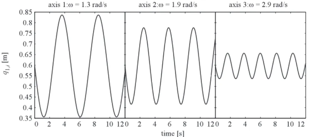
Figure 7.Harmonic displacement profiles used for model verification.

Such motion has been chosen in order to investigate a signif-icant part of the robot workspace, pushing the machine to the physical limits given by the maximum velocity that the three motors are able to perform, which is 0.6 m s−1_.

Results of both virtual and mathematical models are used for computation of the relative difference subsisting between the two sets of forces. In particular, named the maximum ab-solute value of force recorded for motor i during multibody simulations, for the i-th axis it is defined the errorǫias:

ǫi=|

τv,i−τm,i| |τv,i|max

(48)

where τv,i and τm,i are the instantaneous forces computed by multibody environment and mathematical model respec-tively. Equation (48) gives an idea of the deviation between the two methods and therefore it represents a sort of mea-sure of the error introduced by the mathematical model. As visible in Fig. 8, this error never overcomes the 1.0 % of the maximum force during simulation, while the average error is always lower than 1 %.

According to Eq. (47), the actuation forces evaluated dur-ing the previous inverse dynamics simulation can be split in order to analyse the contribution of each part of the robot dynamics. Figure 9 shows the different contributions of the model on the total effort provided by each motor: as well visible, the most part of the force is due to the gravity ac-celeration acting on robot bodies while a negligible contribu-tion is given by Coriolis and centripetal acceleracontribu-tions. This important information can be used during the realization of simplified mathematical models in which, the contribution of force vectorτVcan be ignored.

7 Simulations results

In this section, simulations are shown in order to test the reli-ability of the introduced model in actually reproducible con-ditions.

The first simulation approached is a linear trajectory in-side the workspace. The robot, starting from its home

posi-tion, moves to a given point in the space. The trajectory has been planned in order to obtain continuity on platform accel-erations. The maximum velocity reached by the manipulator is 0.6 m s−1 _{(which corresponds to the maximum linear}

ve-locity available for the actuated joints), while the maximum acceleration is 1.40 m s−2_{. The starting and the ending points}

of the motions are 0.5 m apart; it should be remarked that the robot workspace is a cube with a 0.6 m edge. Thus, the trajec-tory spans a relevant distance with respect to the maximum displacements that the manipulator is able to perform.

For this motion, the forces computed thanks to Eq. (47) are shown in Fig. 10. Also in this case, the most important con-tribution to motors total effort is given by the gravity acceler-ation, while the part of force due to Coriolis and centripetal acceleration is negligible.

A second simulation has been performed with a different trajectory in the space. In this case, the end-effector has been moved from its home configuration to a point in the space. From that point, a horizontal circular trajectory (with diam-eter equal to 0.3 m) centred on robot vertical axis has been performed. Also in this case, the trajectory planning has been performed in order to obtain triangular profiles of accelera-tion. In this case the maximum velocity reached by the mov-ing platform is 0.6 m s−1_{, with a maximum acceleration of}

0.75 m s−2.

Also for this motion, forces profiles are shown (see Fig. 11). Again, the gravity contribute to the total effort is prevailing with respect toτMandτV. The influence ofτV, in particular, represents a negligible contribution to total actua-tion effort. Nevertheless, Fig. 11 shows thatτMconsiderably contributes to the total effort being_|τM,i|max≃20 %|τi|max.

Figure 8.Difference between multibody model and mathematical model.

Figure 9.Different contributions to the total actuation efforts.

Figure 11.Different contributions to the total actuation efforts during a horizontal circular motion.

Figure 12.Different contributions to the total actuation efforts during a horizontal circular motion at maximum allowed thrust.

previous one. In this case the circle owns a diameter of 0.1 m and the manipulator is moved with a constant linear speed of 0.6 m s−1. Also the initial velocity has been taken equal to 0.6 m s−1 in order to overlook effects due to acceleration ramps. Figure 12 shows that forcesτMare in this simulation comparable withτG demonstrating that a control based on the dynamic model can actually improve the performances of the 3-CPU robot. Moreover, Fig. 12 also confirms that the Coriolis terms are negligible and so they may be omitted in a simplified model (from Eq. 47,τ_{≃ −M (qa) ¨qa−G (qa)).}

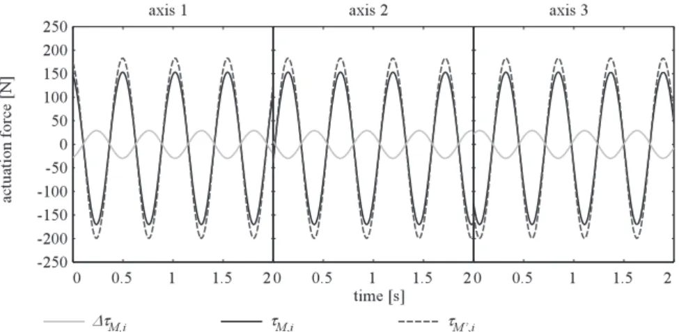
Even though the elimination of the Coriolis terms signifi-cantly lightens the dynamics formulation, further simplifica-tions can be carried on the matrix M itself. As an example, it is presented here the results obtained by the elimination of the terms out of the diagonal of such matrix. In particular, Fig. 13 shows the behaviour ofτM andτM′ for the circular

motion just presented in Fig. 12;τM andτM′ are computed

as:

τ_{M=M (qa) ¨qa} τ_M′=M′_(q

a) ¨qa (49)

where the matrix M′is the simplified M matrix:

M′=          

M1,1 0 0

0 M2,2 0

0 0 M3,3

         

(50)

Figure 13 shows that the use of matrix M′ _{overestimates}

the effect of the mass matrix on the robot dynamics of a maximum value of 30 N (see curve∆τM,i). The error between τMandτM′is here estimated as:

ǫM,i=|

τM,i−τM′,i| max_|τM,i|

(51)

Figure 14 shows the error ǫM for each motor: the graphic shows that the error does not overcome the value of 18 %.

8 Conclusions

Figure 13.Mass matrix contribution to the dynamics in case of plain and simplified model.

Figure 14.Difference between contributions of full mass matrix M and diagonalized mass matrix M′_.

The dynamics of the I.Ca.Ro. manipulator was worked out by means of a virtual work principle approach. The resulting model has been verified through simple simulations, taking advance of a multibody model of the robot. Such verification pointed out that the error subsisting between the two virtual models never overcomes the 1.0 % of the maximum value of torque involved into the motion.

At last, two simulations have been performed on two tra-jectories with main aim of investigating the different contri-butions to the dynamics model. Observation of the results of such simulations yielded a further investigation on the con-tribution to the whole motors efforts. Such study pointed out that the robot is poorly affected by Coriolis and centrifugal forces while the influence of the mass matrix is not negligi-ble. It is author thought that the compensation of this effect by means of a model based control may improve the perfor-mances of robot I.Ca.Ro.

The implementation of the mass matrix on a control algorithm may represent a low efficiency step of a control algorithm because of the heavy mathematical formulation. Due to this, authors also presented a simple simplification of the model based on a simplification of the mass matrix.

Simulations demonstrated that such assumption yield an error that never overcomes the 18 % in a situation of high motors stress.

Edited by: A. Tasora

Reviewed by: L. Bruzzone and one anonymous referee

References

Abdellatif, H. and Heimann, B.: Computational efficient inverse

dynamics of 6-DOF fully parallel manipulators by using the Lagrangian formalism, Mech. Mach. Theory, 44, 192–207,

doi:10.1016/j.mechmachtheory.2008.02.003, 2009.

Caccavale, F., Siciliano, B., and Villani, L.: The

Tri-cept robot: dynamics and impedance control,

Mecha-tronics, IEEE/ASME Transactions on, 8, 263–268,

doi:10.1109/TMECH.2003.812839, 2003.

Callegari, M. and Palpacelli, M.-C.: Prototype design of a

translat-ing parallel robot, Meccanica, 43, 133–151, doi:10.1007/

s11012-008-9116-8, doi:10.1007/s11012-008-9116-8, 2008.

Carbonari, L. and Callegari, M.: The kinematotropic 3-CPU parallel robot: analysis of mobility and reconfigurability aspects, in: Lat-est Advances in Robot Kinematics, edited by: Lenarˇciˇc, J. and Husty, M., Springer, 2012.

Carbonari, L., Callegari, M., Palmieri, G., and Palpacelli, M.: A new class of reconfigurable parallel kinematics machines, Mech. Mach. Theory, in review, 2013.

Dasgupta, B. and Mruthyunjaya, T.: A Newton-Euler formulation for the inverse dynamics of the Stewart platform

manipula-tor, Mech. Mach. Theory, 33, 1135–1152, doi:10.1016/

S0094-114X(97)00118-3, 1998.

Daun, Q., Daun, B., and Daun, X.: Dynamics modelling and hy-brid control of the 6-UPS platform, in: 2010 International Con-ference on Mechatronics and Automation (ICMA), 434 –439,

doi:10.1109/ICMA.2010.5589105, 2010.

Di Gregorio, R. and Parenti-Castelli, V.: Dynamics of a Class of Parallel Wrists, J. Mech. Design, 126, 436–441,

doi:10.1115/1.1737382, 2004.

Do, W. Q. D. and Yang, D. C. H.: Inverse dynamic analysis and simulation of a platform type of robot, J. Robotic Syst., 5, 209–

227, doi:10.1002/rob.4620050304, 1988.

Gallardo, J., Rico, J., Frisoli, A., Checcacci, D., and Bergamasco, M.: Dynamics of parallel manipulators by means of screw

the-ory, Mech. Mach. Thethe-ory, 38, 1113–1131, doi:10.1016/

S0094-114X(03)00054-5, 2003.

Khalil, W. and Ibrahim, O.: General Solution for the Dynamic Mod-eling of Parallel Robots, J. Intell. Robotics Syst., 49, 19–37,

doi:10.1007/s10846-007-9137-x, 2007.

Kovecses, J., Piedboeuf, J. C., and Lange, C.: Dynamics modeling and simulation of constrained robotic systems,

Mechatronics, IEEE/ASME Transactions on, 8, 165–177,

doi:10.1109/TMECH.2003.812827, 2003.

Kunquan, L. and Rui, W.: Closed-form Dynamic Equations of the 6-RSS Parallel Mechanism through the Newton-Euler Approach, in: 2011 Third International Conference on Measuring Tech-nology and Mechatronics Automation (ICMTMA), 1, 712–715,

doi:10.1109/ICMTMA.2011.180, 2011.

Lin, Y.-J. and Song, S.-M.: A comparative study of inverse dynam-ics of manipulators with closed-chain geometry, J. Robotic Syst.,

7, 507–534, doi:10.1002/rob.4620070402, 1990.

Lopes, A. M.: Dynamic modeling of a Stewart platform using the generalized momentum approach, Commun. Nonlinear Sci., 14,

3389–3401, doi:10.1016/j.cnsns.2009.01.001, 2009.

Miller, K.: Optimal Design and Modeling of Spatial

Par-allel Manipulators, Int. J. Robot. Res., 23, 127–140,

doi:10.1177/0278364904041322, 2004.

Moon, F.: Applied Dynamics: With Applications to Multibody and Mechatronic Systems, John Wiley & Sons, 2008.

Papastavridis, J.: Analytical Mechanics: A Comprehensive Trea-tise on the Dynamics of Constrained Systems, World Scientific, 2012.

Tsai, L.-W.: Solving the Inverse Dynamics of a Stewart-Gough Ma-nipulator by the Principle of Virtual Work, J. Mech. Design, 122,

3–9, doi:10.1115/1.533540, 2000.

Wang, J. and Gosselin, C. M.: A New Approach for the Dynamic Analysis of Parallel Manipulators, Multibody Syst. Dyn., 2, 317–

334, doi:10.1023/A:1009740326195, 1998.

Wang, J., Wu, J., Wang, L., and Li, T.: Simplified strategy of the dynamic model of a 6-UPS parallel kinematic machine for real-time control, Mech. Mach. Theory, 42, 1119–1140,

doi:10.1016/j.mechmachtheory.2006.09.004, 2007.

Wronka, C. and Dunnigan, M.: Derivation and analysis of a dy-namic model of a robotic manipulator on a moving base, Robot.

Auton. Syst., 59, 758–769, doi:10.1016/j.robot.2011.05.010,

2011.

Yang, C., Han, J., Zheng, S., and Ogbobe Peter, O.: Dynamic

modeling and computational efficiency analysis for a spatial

6-DOF parallel motion system, Nonlinear Dynam., 67, 1007–1022,

doi:10.1007/s11071-011-0043-1, 2012.

Zhang, C.-D. and Song, S.-M.: An efficient method for inverse

dy-namics of manipulators based on the virtual work principle, J.