GOMOS data characterization and error estimation

(1)

ACPD

10, 6755–6796, 2010

GOMOS data characterization

J. Tamminen et.al

Title Page

Abstract Introduction

Conclusions References

Tables Figures

◭ ◮

Back Close

Full Screen / Esc

Printer-friendly Version

Interactive Discussion Atmos. Chem. Phys. Discuss., 10, 6755–6796, 2010

www.atmos-chem-phys-discuss.net/10/6755/2010/ © Author(s) 2010. This work is distributed under the Creative Commons Attribution 3.0 License.

Atmospheric Chemistry and Physics Discussions

This discussion paper is/has been under review for the journal Atmospheric Chemistry and Physics (ACP). Please refer to the corresponding final paper in ACP if available.

GOMOS data characterization and error

estimation

J. Tamminen1, E. Kyr ¨ol ¨a1, V. F. Sofieva1, M. Laine1, J.-L. Bertaux2,

A. Hauchecorne2, F. Dalaudier2, D. Fussen3, F. Vanhellemont3,

O. Fanton-d’Andon4, G. Barrot4, A. Mangin4, M. Guirlet4, L. Blanot4, T. Fehr5,

L. Saavedra de Miguel5, and R. Fraisse6

1

Finnish Meteorological Institute, Earth Observation, Helsinki, Finland 2

Service d’Aeronomie, Paris, France 3

BIRA-IASB, Brussels, Belgium 4

ACRI ST, Sophia Antipolis, France 5

ESA-ESRIN, Italy 6

EADS-Astrium, Toulouse, France

Received: 31 January 2010 – Accepted: 26 February 2010 – Published: 11 March 2010

Correspondence to: J. Tamminen (johanna.tamminen@fmi.fi)

(2)

ACPD

10, 6755–6796, 2010

J. Tamminen et.al

Title Page

Tables Figures

◭ ◮

Back Close

Full Screen / Esc

Interactive Discussion

Abstract

The Global Ozone Monitoring by Occultation of Stars (GOMOS) instrument uses stellar occultation technique for monitoring ozone and other trace gases in the stratosphere and mesosphere. The self-calibrating measurement principle of GOMOS together with a relatively simple data retrieval where only minimal use of a priori data is required,

5

provides excellent possibilities for long term monitoring of atmospheric composition. GOMOS uses about 180 brightest stars as the light source. Depending on the in-dividual spectral characteristics of the stars, the signal-to-noise ratio of GOMOS is changing from star to star, resulting also varying accuracy to the retrieved profiles. We present the overview of the GOMOS data characterization and error estimation,

10

including modeling errors, for ozone, NO₂, NO₃and aerosol profiles. The retrieval er-ror (precision) of the night time measurements in the stratosphere is typically 0.5–4% for ozone, about 10–20% for NO2, 20–40% for NO3 and 2–50% for aerosols.

Meso-spheric O₃, up to 100 km, can be measured with 2–10% precision. The main sources of the modeling error are the incompletely corrected atmospheric turbulence causing

15

scintillation, inaccurate aerosol modeling, uncertainties in cross sections of the trace gases and in the atmospheric temperature. The sampling resolution of GOMOS varies depending on the measurement geometry. In the data inversion a Tikhonov-type reg-ularization with pre-defined target resolution requirement is applied leading to 2–3 km resolution for ozone and 4 km resolution for other trace gases.

20

1 Introduction

Vertical profiles of stratospheric constituents have been measured using satellite in-struments since 1979 when SAGE I (Stratospheric Aerosol and Gas Experiment I), the first instrument of the successful SAGE family, started to operate. The solar occulta-tion technique that was used by the SAGE instruments has turned out to be a reliable

25

(3)

ACPD

10, 6755–6796, 2010

J. Tamminen et.al

Title Page

Tables Figures

◭ ◮

Back Close

Full Screen / Esc

Interactive Discussion the SAGE series, have utilised the same technique at various wavelenght regions

in-cluding ATMOS, SAM II, HALOE, POAM series, ACE-mission and SCIAMACHY. The success story of the solar occultation technique goes on and recently launched so-lar occultation instruments SOFIE (Soso-lar occultation for Ice Experiment) on board AIM satellite and SEE (Solar EUV Experiment) on board TIMED satellite are targeted for

5

studying the mesospheric and thermospheric composition, respectively.

In addition to sun also stars can be used as a light source when studying the com-position of the atmosphere. This was theoretically demonstrated by Hays and Roble (1968) and later also shown in practice. In 1996 US launched MSX satellite with UVISI instrument on-board, which performed several stellar occultation measurements and

10

demonstrated the potential of the technique to study globally the atmospheric com-position and temperature despite that it was not designed for that particular purpose (Yee et al., 2002; Vervack et al., 2003). For a more comprehensive summary of the occultation instruments see Bertaux et al. (2010).

The first instrument specifically developed for studying the composition of the

at-15

mosphere by utilizing the stellar occultation technique is European Space Agency’s GOMOS (Global Ozone Monitoring by Occultation of Stars) instrument on-board the Envisat satellite, launched in March 1st 2002 (Bertaux et al., 2004; Kyr ¨ol ¨a et al., 2004; Bertaux et al., 2010). GOMOS is a ultraviolet-visible spectrometer that covers wave-lengths from 250 nm to 675 nm with 1.2 nm resolution and in addition two infrared

chan-20

nels at 756–773 nm and 926–952 nm with 0.2 nm resolution. Two photometers that are located at blue (473–527 nm) and red (646–698 nm) measure the stellar flux through the atmosphere at a sampling frequency of 1 kHz. By August 2009 GOMOS had ob-served about 668 000 stellar occultations. An overview of the GOMOS instrument and highlights of the measurements are given in Bertaux et al. (2010)

25

(4)

ACPD

10, 6755–6796, 2010

J. Tamminen et.al

Title Page

Tables Figures

◭ ◮

Back Close

Full Screen / Esc

Interactive Discussion coverage. Compared to the solar occultation, stars are point-like sources that result in

an excellent pointing information. The disadvantage compared to the solar occultation is the signal-to-noise ratio that is much lower in the stellar occultation technique.

GOMOS is following about 180 different stars while they are descending behind the Earth limb. Since the stars are different both in brightness (magnitude) and in the

5

spectrum of the light (originating from stellar properties and surface temperature) also the data characteristics measured by GOMOS vary strongly. Even without taking the atmospheric impact into account, the signal-to-noise ratio varies strongly from star to star. In this respect, one might even consider GOMOS being a remote sensing mission that consists of 180 different instruments each having its own data characteristics.

10

The importance of the data characterization and the error estimation is nowadays widely recognized (see e.g., Rodgers, 2000). The further utilization of the remote sensed data, e.g., in the assimilation or in constructing time series, depends crucially on a proper error characterization. The purpose of this paper is to characterize the quality of the GOMOS night time data products. Both systematic errors and random

15

errors are considered. The results shown here are based on estimating the impact of various assumptions that are made in the GOMOS data processing. The GOMOS Level 1b and Level 2 data processing are described in details in Kyr ¨ol ¨a et al. (2010). A review of the geophysical validation of GOMOS data products is included in Bertaux et al. (2010).

20

In this paper, we characterize O3, NO2, NO3and aerosol profiles that are retrieved

from GOMOS UV-VIS spectrometer data at the altitude range 10–100 km during the night time. Only dark limb (night) occultations, i.e., occultations with solar zenith angle larger than 107 deg, are considered. The bright limb occultations (i.e., made during day time) are not considered here since the data quality in these measurements is much

25

(5)

ACPD

10, 6755–6796, 2010

J. Tamminen et.al

Title Page

Tables Figures

◭ ◮

Back Close

Full Screen / Esc

Interactive Discussion necessary, the difference in IPF Version 5 and 6 data. General features of GOMOS

measurements are given in Sect. 2. The propagation of the random measurement error through the retrieval steps are discussed in Sect. 3. The contribution of vari-ous modelling errors are discussed in Sect. 4. The vertical resolution is discussed in Sect. 5. The precision of the retrieved profiles varies strongly from occultation to

occul-5

tation and this is discussed in Sect. 6, where we give examples of the GOMOS error estimates and discuss the valid altitude range of the profiles. Finally, we summarize the most important sources of random and systematic errors in Sect. 7.

2 GOMOS spectral measurements and their characteristics

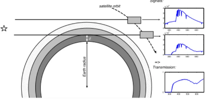
2.1 Signal-to-noise ratio

10

GOMOS measures the stellar light through the atmosphere as the stars set behind the Earth limb. However, stars are not similar and this has an impact on GOMOS results as well. The most significant characteristic related to the stellar occultation technique is that the accuracy of the retrieved parameters depends strongly on the stellar prop-erties.The measured stellar signal and further the transmission which is used as the

15

data in the GOMOS retrievals varies strongly depending on the stellar brightness and temperature. This is illustrated in Fig. 2, where examples of the GOMOS transmission spectrum at different altitudes (10–70 km) are shown for different stars (bright and cool, bright and hot, dim and cool and dim and hot). We observe clearly that the data using dim stars are much noisier compared to using bright stars. In addition, the stellar

tem-20

perature has an impact: hot stars have the maximum intensity of the radiation at UV wavelengths whereas cool stars have the maximum at the VIS wavelengths and the UV part is very noisy.

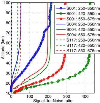
In Fig. 3 the GOMOS signal-to-noise ratio at 3 different wavelenght regions (UV and 2 visible) are shown in three cases: Sirius (the brightest star, star number 1 in GOMOS

25

(6)

ACPD

10, 6755–6796, 2010

J. Tamminen et.al

Title Page

Tables Figures

◭ ◮

Back Close

Full Screen / Esc

Interactive Discussion cool star (star number 4, Mv=−0.01, T=58 00 K) and dim and cool star (star number

117, Mv=2.7, T=38 00 K). When retrieving ozone at high altitudes, above 40 km, the

Hartley band (248–310 nm) is crucial and at this altitude region the hot stars provide significantly better results than the cool stars. The average SNR of GOMOS at UV around 50 km using Sirius is 130–160 whereas using cool stars (T <6000 K, stars 4

5

and 117 in Fig. 3) the SNR is close to zero. At lower altitudes, where the retrieval is most sensitive to Chappuis band at visible wavelengths both hot and cool stars are, in general, equally good. For NO₃ the situation is quite the opposite. The strongest NO3 signal comes from visible wavelengths around 660 nm, hence the cool stars are

slightly more favourable for NO3retrieval. Aerosols and NO2are retrieved mainly below

10

50 km using a wide spectral window and therefore the retrievals do not have significant dependence on the stellar temperature.

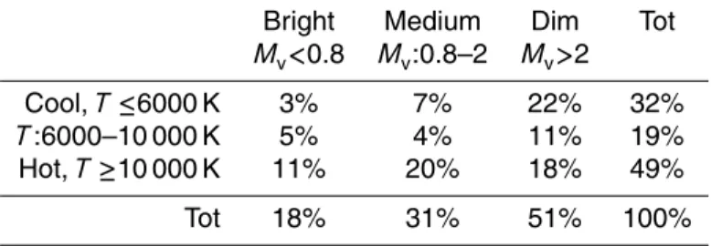
Statistics of the stellar characteristics in the night time occultations during years 2002–2008 are given in Table 1. The occultations are divided into nine categories depending the stellar brightness and temperature. Roughly two thirds of the

occulta-15

tions are performed using either hot or medium temperature stars and about half using either bright or medium brightness stars.

2.2 Spatio-temporal distribution of GOMOS measurements

2.2.1 Mission planning

As the light source GOMOS uses about 180 brightest stars with stellar magnitude

20

brighter than 3 (Mv<3). As there are often several stars available simultaneously in

the GOMOS field-of-view some prioritization needs to be made. The purpose of the GOMOS mission planning is to select for each orbit the optimal set of 25–40 stars that will be used for occultation measurements. About half of the occultations are made in night time. The optimization is done using several criteria, like the geographical

25

(7)

ACPD

10, 6755–6796, 2010

J. Tamminen et.al

Title Page

Tables Figures

◭ ◮

Back Close

Full Screen / Esc

Interactive Discussion The selected set of stars is to large extent repeated for several orbits until the stars

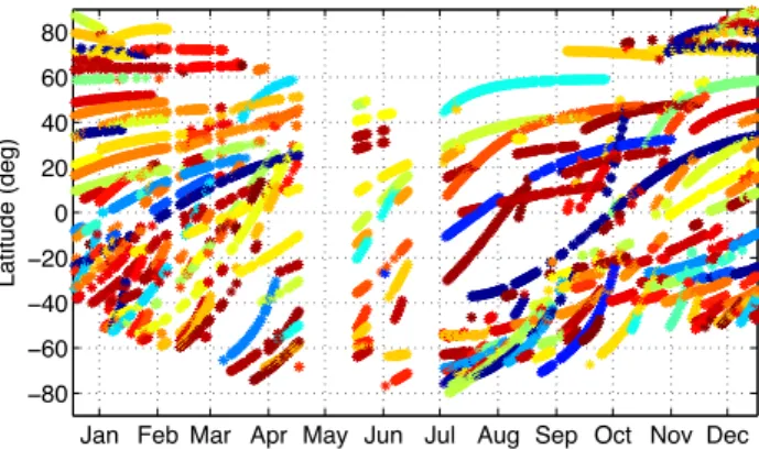
are out of the field-of-view. Occultations of the same star at successive orbits are made at the same latitude band but with varying longitude (about 15/day). In Fig. 4 the latitude coverage of the night time occultations during 2003 are shown. The individual stars can typically be followed for several months in a row.

5

2.2.2 Geographical distribution of GOMOS measurements

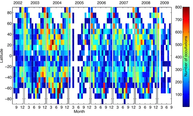
The GOMOS measurements cover the whole globe from pole to pole. This can be seen in Fig. 5 where the geographical distribution of the GOMOS night time measure-ments from summer 2002 to autumn 2009 are shown. We see that quite a good global coverage can be obtained using 10 deg latitude bands. In particular, the unique

mea-10

surements of GOMOS during polar night have been utilized extensively e.g., in studies of long term e_ffects of solar proton events during polar night (Sepp ¨al ¨a et al., 2007; Verronen et al., 2005) and in studying the effect of intense warming and air descent Hauchecorne et al. (2007).

Depending on the season, there is some variation in the distribution of the

measure-15

ments as the stars are not distributed evenly in the sky (see Fig. 5). In addition, the night time measurements do not cover the summer pole. The calibration measure-ments that are performed at each orbit close to the equator cause some reduction in the number of occultations there.

The yearly variations in the measurement distribution are caused by technical

prob-20

lems in the instrument. In May 2003 there was a technical anomaly and the number of measurements was low during May and June in 2003. After another technical anomaly that took place in January 2005 the viewing angle was slightly reduced and the num-ber of (night-time) profiles went down from about 200 to 150 profiles per day. In 2009 the number of occultations has been clearly less than in the previous years and this is

25

(8)

ACPD

10, 6755–6796, 2010

J. Tamminen et.al

Title Page

Tables Figures

◭ ◮

Back Close

Full Screen / Esc

Interactive Discussion In principle, GOMOS measures each year the same stars at the same latitude

re-gions which is very useful when making a time series analysis based on the data. Some changes have, however, taken place during the mission due to the reduced viewing an-gle. Moreover, it is important to keep in mind that there are differences in the overall global coverage and some latitude bands are covered more densely that the others.

5

2.2.3 Altitude range

The GOMOS instrument is equipped with the star tracker operating at 625–950 nm, which follows the star by keeping the image of the star in the centre of the slit. The technique has turned out to work reliably (except the last technical anomaly in 2009) and the stars can typically be tracked from the top of the atmosphere (120–150 km)

10

down to 5–20 km tangent altitude. It seems that when no clouds are present, stars can be followed as low as 5 km altitude (especially bright stars). The presence of clouds in the field-of-view leads to loosing the signal. Other factors affecting the lowest altitude are stellar brightness (the brighter the star, the lower the tangent altitude) and regular refraction (the star image can fall outside the field-of-view due to refraction). Figure 6

15

shows the lowest measurement altitude for 30 brightest stars (with visual magnitudes<

1.6). This distribution is in very good general agreement with the maps of the cloud top height (e.g., http://isccp.giss.nasa.gov/index.html), thus indicating that the main reason for terminating the occultations of bright stars is the presence of clouds. In tropics, the lowest altitude is 15–18 km because of frequent presence of high clouds (cirrus and

20

convective clouds). Above South Pole the measurements are also often terminated at 15–18 km, most probably because of frequent occurrence of polar stratospheric clouds (note that polar regions are not covered by GOMOS in summer). The lowest altitude in occultations of bright stars can potentially provide valuable information about cloud top height.

(9)

ACPD

10, 6755–6796, 2010

J. Tamminen et.al

Title Page

Tables Figures

◭ ◮

Back Close

Full Screen / Esc

3 Error propagation through GOMOS retrieval

The random error plays an important role in the GOMOS total error budget, unlike what is the case in several other remote sensing instruments which are dominated by sys-tematic errors. The random errors in GOMOS data are mainly due to the propagation of the measurement noise and the imperfect scintillation correction. First we discuss

5

how the measurement noise is propagated through the GOMOS retrieval steps. The GOMOS retrieval procedure is described in details in Kyr ¨ol ¨a et al. (2010) and we will use here the same notation as much as possible.

The GOMOS data retrieval is based on describing the measurement and the quan-tities to be retrieved as random variables. By error propagation we mean how the

10

measurement noise and possible modelling errors impact the uncertainty of the re-trieved quantities. In the GOMOS retrieval procedure we apply the Bayesian theorem and describe the solution asa posteriori distributionwhich is in practice approximated with Gaussian distribution whose mode and covariance are computed. The covariance matrix describes the uncertainty of the retrieved quantities.

15

3.1 Error propagation through spectral inversion

The GOMOS retrieval problem is solved in two steps which are calledspectral inversion andvertical inversion. In spectral inversion horizontally integrated column densities of O₃, NO₂, NO₃ and aerosols are simultaneously fitted to the transmission data T_extobs

(which is corrected for refractive effects, see Eq. (32) in Kyr ¨ol ¨a et al., 2010).

Measure-20

ments at successive tangent altitudes are treated separately. Assuming that the noise in the transmission is Gaussian, the problem of finding maximum a posteriori point is equal with finding the solution that minimizes the sum of squared residuals term: SSR=(Text−Textobs)C

−1

(Text−Textobs)

T ₍₁₎

whereTextrefers to the modelled transmission which depends on the horizontally

inte-25

(10)

ACPD

10, 6755–6796, 2010

J. Tamminen et.al

Title Page

Tables Figures

◭ ◮

Back Close

Full Screen / Esc

Interactive Discussion Kyr ¨ol ¨a et al. (2010). The covariance matrixC includes both measurement and

mod-elling errors. In the present GOMOS processing (IPF Version 5) the modmod-elling error is ignored, but in the updated version (IPF Version 6) this is also taken into account (see Sect. 4.1). The inverse problem is non-linear and it is solved iteratively by applying Levenberg-Marquardt algorithm (Press et al., 1992). The algorithm assumes that the

5

posterior distribution is roughly Gaussian close to the point that minimizes the sum of squared residuals, so that the posterior distribution of the horizontal column densities can characterized with the estimate and the covariance matrixC_N. The posterior co-variance matrix is also returned by the Levenberg-Marquardt algorithm. The diagonal elements of the covariance matrix characterize the variance of the error estimates of

10

the horizontal column densities.

Instead of using a fast iterative algorithm one can apply more time consuming Monte Carlo methods to compute the real posterior distribution to analyse the validity of the assumption of Gaussian posterior distribution. The Markov chain Monte Carlo (MCMC) technique has been successfully applied to the GOMOS spectral inversion (Tamminen

15

and Kyr ¨ol ¨a, 2001; Tamminen, 2004). It has been shown that Gaussian posterior distri-bution is a good approximation in the GOMOS spectral inversion (Tamminen, 2004).

3.1.1 Correlated errors after spectral inversion

The absorption cross sections of gases and aerosols are not independent and there-fore the retrieval errors of these constituents can also be correlated. The amount of

20

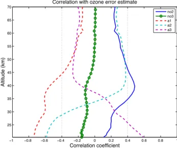
correlation changes depending on the altitude due to the changing effective wave-length region. The off-diagonal values of the posterior covariance matrixC_N describe the correlations in the errors. In Fig 7 we give an example of the the correlation coef-ficients (R_N(i ,j)=C_N(i ,j)/p(C_N(i ,i)C_N(j,j))) between the errors in O₃ and the other retrieved parameters (NO2, NO3, and three aerosol parameters) after the spectral

in-25

version. In the figure, the correlation coefficients are plotted for all retrieval altitudes. We note that, in this case, the error estimates of the horizontally integrated column O3

(11)

ACPD

10, 6755–6796, 2010

J. Tamminen et.al

Title Page

Tables Figures

◭ ◮

Back Close

Full Screen / Esc

Interactive Discussion 25 km. Some positive correlation with O₃ and NO₂ column errors can also be seen,

but that is generally below 0.4. The maximum correlation (∼0.5) seems to be around 20–40 km depending on the stellar type and the atmospheric composition. The cor-relation between O₃ and NO₃is negligible. The correlation structure varies somewhat depending on the stellar characteristics and the example given in Fig. 7 corresponds

5

to a hot star.

In principle, the correlation in errors should be taken into account when analysing, e.g., the correlations of gases. However, this is typically not done, and in GOMOS case this information is not available for profiles but only for horizontally integrated column densities after the spectral inversion. A simplified simulation study was performed in

10

order to get an idea how much the correlated errors impact if we want to estimate the correlation of the gases (e.g., O3and NO2). The study showed that the estimated

cor-relation of the gases was only very slightly biased when the corcor-relation in their errors was not taken into account. However, the accuracy of the estimated correlation of the gases was more influenced. Based on this exercise we can conclude that when using

15

GOMOS data to study correlation between O3 and NO2 or aerosols the significance

of the correlation may be either overestimated or underestimated. If the correlation we found is negative/positive and the errors are also correlated negatively/positively then the significance of the correlation is underestimated and if the errors are correlated dif-ferently, positively/negatively, then the significance of the correlation is overestimated.

20

3.1.2 Random error propagation through vertical inversion

In the vertical inversion the horizontally integrated column densities are transformed to local densities using information about the ray path of the measurement. Each con-stituent is treated separately and the correlations between the errors of the horizontal column densities are not taken into account, see Kyr ¨ol ¨a et al. (2010) for description.

25

(12)

ACPD

10, 6755–6796, 2010

J. Tamminen et.al

Title Page

Tables Figures

◭ ◮

Back Close

Full Screen / Esc

Interactive Discussion after the spectral inversion. Now the covariance matrix of the retrieved profile is simply

Cρ=LCNL

T_, ₍₂₎

whereLis the retrieval matrix so thatρ=LN (corresponding to Eq. (49) in Kyr ¨ol ¨a et al. (2010)). The diagonal elements of of the posterior covariance matrixCρdescribe the variance of the estimated local density values whereas the off-diagonal elements of

5

the covariance matrixC_ρcharacterize the correlation between the retrieved densities at successive layers. In GOMOS data products six most significant off-diagonal ele-ments are reported. After applying the Tikhonov regularization the errors of the nearby layers are somewhat correlated, see Fig. 8 where the correlation coefficients for the ozone retrieval (R_ρ(i ,j)=C_ρ(i ,j)/p(C_ρ(i ,i)C_ρ(j,j))) are plotted for five selected

alti-10

tudes. We see that, above 35 km where the Tikhonov regularization is stronger, also the correlation in the errors is larger, and involves about 3 layers above and below the retrieval height. Below 30 km only errors from 2 layers below and above the retrieval altitude are slightly correlated. In oblique occultations there is a larger correlation be-tween the errors at neighbouring layers because the regularization is stronger than in

15

the vertical occultations.

4 Modelling errors

In the GOMOS retrieval the faint signal is compensated by using a wide spectral win-dow for the data processing. The advantage is clear – we maximize the use of the data, but, as a drawback, the consistency in the modelling of the wide wavelength

20

band becomes much more important. In the GOMOS spectral inversion residuals (i.e., measured transmission spectra minus modelled ones) we see some structures which are mainly due to imperfect scintillation correction. They are considered as the largest modelling error in the GOMOS retrieval. The imperfect modelling of the aerosol con-tribution is an important source of modelling error especially at low altitudes. Other

(13)

ACPD

10, 6755–6796, 2010

J. Tamminen et.al

Title Page

Tables Figures

◭ ◮

Back Close

Full Screen / Esc

Interactive Discussion sources of modelling error are uncertainties in the absorption cross sections and

tem-perature. Relatively negligible impact is seen due to uncertainty of neutral density profile, ray path computation and potentially missing constituents.

4.1 Scintillation – dilution correction

When the stellar light traverses through the atmosphere, it is affected also by the

re-5

fractive effects, dilution and scintillation, which need to be taken into account in the retrieval. The approach taken in the GOMOS data processing is to remove these ef-fects before performing the inversion (see Kyr ¨ol ¨a et al., 2010 for general description of the algorithms).

The dilution term is approximated using ECMWF air density. As the refraction can be

10

accurately computed, the error caused by this assumption is negligible in the retrieved profiles (Sofieva et al., 2006).

In the GOMOS retrievals, the perturbations in the stellar flux caused by scintillations are corrected by using additional scintillation measurements by the fast photometer operating in low-absorption wavelength region (Dalaudier et al., 2001; Sofieva et al.,

15

2009). The quality of the scintillation correction and its limitations are discussed in Sofieva et al. (2009) where it was shown that the applied scintillation correction re-moves significant part of the perturbations in the recorded stellar flux caused by scintil-lations, but it is not able to remove scintillations generated by the isotropic turbulence. The remaining perturbations, due to the incomplete scintillation correction, are not

neg-20

ligible: in oblique occultations of bright stars, they can be comparable or even exceed the instrumental noise by a factor of 2–3 at the altitude 20–45 km (Sofieva et al., 2009) (Fig. 9). This causes about 0.5–1.5% additional error in the ozone retrievals at the altitude range of 20–45 km (Sofieva et al., 2009).

The modelling error caused by the imperfect scintillation correction can be taken into

25

(14)

ACPD

10, 6755–6796, 2010

J. Tamminen et.al

Title Page

Tables Figures

◭ ◮

Back Close

Full Screen / Esc

Interactive Discussion on statistical analyses of GOMOS residuals and the theory of isotropic scintillations,

the scintillation correction error is assumed to be a Gaussian random variable with zero mean and a non-diagonal covariance matrix (Sofieva et al., 2009). When the scintillation correction errors are taken into account, the normalizedχ2 values which reflect the agreement between the measurement and modelling become close to the

5

optimal value 1. This improvement ensures that the estimated accuracy of the retrieved profiles is closer to the reality after including the modelling error component to the retrieval. In the present operational GOMOS Level 2 algorithm (IPF Version 5) this is not included, but it will be implemented in the new IPF Version 6 in spring 2010.

The incomplete scintillation correction is the main source of GOMOS modelling

er-10

rors in the stratosphere (at altitudes 20–45 km). However, this modelling error is not systematic but random in nature. By averaging measurements on successive layers or requiring smoothness of the retrieved profile (as is done in GOMOS vertical inversion) the impact of this modelling error reduces.

4.2 Uncertainty in aerosol modelling

15

In the GOMOS spectral inversion absolute cross sections are used and the aerosols are also inverted simultaneously with the trace gases. The aerosol cross sections de-pend on the aerosol size distribution and composition which are unknown. A practical approach is to use a simplified wavelength dependent model for the aerosol cross sec-tions. In the present algorithm, aerosol cross sections are assumed to depend on the

20

wavelength, λ, according to a second order polynomial (see Kyr ¨ol ¨a et al., 2010 for details of the algorithm). Three parameters are fitted. The choice of using second or-der polynomial is somewhat arbitrary and first or third oror-der polynomials could also be considered.

A sensitivity study was made in order to quantify the modelling error caused by using

25

(15)

ACPD

10, 6755–6796, 2010

J. Tamminen et.al

Title Page

Tables Figures

◭ ◮

Back Close

Full Screen / Esc

1

λ. Aerosol model A-3 corresponds to the one that is used in the operational GOMOS data processing IPF (both Versions 5 and 6). As a test case we used took than 1000 occultations and compared the median values in this set, see Fig. 9. These results are obtained using the presently available GOMOS Version 5 processing. We note that the (physically most unrealistic) model A-1 gives quite di_fferent results than the others. By

5

comparing the impact of the other models we can conclude the following. The aerosol model selection has its largest impact at low altitudes below 20 km. For ozone the sensitivity is of the order of 20% below 20 km and 1–5% between 20–25 km. Above 25 km the uncertainty in the aerosol modelling does not have much impact to ozone retrieval. For NO2the impact is typically around 10% between 15–20 km. Above 20 km

10

the impact is small, less than 5%. For NO₃the impact can be as large as 100% around 15–20 km, but above 25 km, which is the lowest reasonable altitude for NO3, it does

not affect the results significantly. The impact in aerosol extinction is below 10% up to 35 km and larger above.

In a recent publication, a technique for selecting the best aerosol model in the

GO-15

MOS spectral inversion is developed using Markov chain Monte Carlo technique (Laine and Tamminen, 2008). It is shown that the model selection can be implemented si-multaneously with the parameter estimation to the spectral inversion. More work is, however, needed to show the quantitative advantage in practice.

4.3 Uncertainty of cross sections and atmospheric temperature

20

The retrieval of the atmospheric constituents from the GOMOS measurements is based on assuming a good knowledge of the cross sections of the retrieved gases O3, NO2

and NO3. See Kyr ¨ol ¨a et al. (2010) for more details of the cross sections that are used in

GOMOS retrievals. The errors in the cross sections are, unfortunately, not well known. Some studies, assuming independent Gaussian distributed uncertainty have been

per-25

formed, but the validity of these estimates is, however, limited, since the uncertainty is not realistically modelled. By comparing several sets of laboratory measured O3cross

(16)

ACPD

10, 6755–6796, 2010

J. Tamminen et.al

Title Page

Tables Figures

◭ ◮

Back Close

Full Screen / Esc

Interactive Discussion absolute values and also in their temperature dependence, and the uncertainties are

not independent (see e.g., Burrows et al., 1999). When the nature of the uncertainty is not known, it is also difficult to take into account in the inverse problem. By making a sensitivity study and using different sets of ozone cross sections in GOMOS spectral inversion we observe a difference of the order of 1–1.5% in ozone retrieval.

5

The absorption cross sections of O3, NO2and NO3depend also on the temperature

and, therefore, some error is also caused by the uncertainty in the atmospheric temper-ature. In some sense, part of the systematic bias in the cross sections could, actually, be modelled as the uncertainty in the temperature. Unlike in several other instruments, in the operational GOMOS retrieval the atmospheric temperature is not fitted but

as-10

sumed to be known. For that ECMWF temperature below 50 km is used and MSIS90 temperature above 50 km. If moderate Gaussian uncertainty (with zero mean and 2 K standard deviation) in the temperature information is taken into account the error in O3

retrieval increases slightly (<0.5%) at 30–60 km altitude range (Tamminen, 2004). At this altitude the retrieval is based on Huggins band where the cross sections are known

15

to be strongly temperature dependent. The impact is less significant with NO2and NO3

retrievals which are more dominated by the random measurement noise.

Further work is still needed to understand the nature of the uncertanties in the cross sections and to properly estimate the impact in the GOMOS products. This work will be contiued as a part of the IGACO-O3/UV activity, initiated by IO3C (International

20

Ozone Commision) and WMO-GAW, on the evaluation of the absoption cross sections of ozone (ACSO, see http://igaco-o3.fmi.fi/ACSO/). This activity, which involves several ground based and satellite instruments using the Huggins band, will be finalized by 2011.

4.4 Uncertainty of neutral density profile

25

In earlier versions of the GOMOS data processing also the neutral density was inverted simultaneously with O3, NO2, NO3and aerosols. Due to the similar nature of Rayleigh

(17)

ACPD

10, 6755–6796, 2010

J. Tamminen et.al

Title Page

Tables Figures

◭ ◮

Back Close

Full Screen / Esc

Interactive Discussion are strongly correlated. In order to improve the aerosol retrieval it was decided to

fix the the neutral density concentration using ECMWF analysis values below 50 km and to use MSIS90 model values above. Assuming, that the uncertainty of ECMWF neutral density is around 2% we observe negligible (<1%) impact for O3, NO2 and

NO₃retrievals. However, in aerosol retrieval the impact is larger. Around 22–40 km the

5

impact is generally around 5–10% (with maximum impact around 27 km 15%). Below 22 km the impact is less significant being smaller than 5%.

4.4.1 Missing constituents

The wavelength band 248–690 nm that is used for retrieval of O₃, aerosols, NO₂ and NO3 contains also absorption by OClO, BrO and Na. However, in individual retrievals

10

their impact is so small that the error caused by not including them in the modelling is negligible. Only by averaging several hundreds of measurements the signatures of, e.g., Na can be seen (Fussen et al., 2004). The wavelengths that include O2signature

at 627–630 nm are excluded from the inversion.

4.5 Uncertainty in ray tracing and measurement position

15

One of the advantages of the stellar occultation technique is that the measurement target is a point source whose position is well known. Therefore, the uncertainty in the ray path and its tangent altitude is only due to the uncertainty in the satellite position and the ray path calculation. The position of the Envisat satellite is also well known so the impact of this uncertainty is rather small, of the order of 30 m (Bertaux et al., 2010).

20

The ray path calculation is done using the ECMWF neutral density analysis data and it causes at maximum about 15 m error in the tangent altitude for ray paths at 10 km altitude range, above that the impact is smaller and<5 m for rays above 20 km altitude (Sofieva et al., 2006).

In conclusion, the uncertainty in the GOMOS measurement ray path cause only

neg-25

(18)

ACPD

10, 6755–6796, 2010

J. Tamminen et.al

Title Page

Tables Figures

◭ ◮

Back Close

Full Screen / Esc

Interactive Discussion studies where no altitude shift has been found (see e.g., Meijer et al., 2004; Bertaux

et al., 2010).

5 Vertical resolution

Due to the stellar occultation measurement principle and measurement geometry the vertical resolution of GOMOS is very good. The sampling resolution of GOMOS is

5

between 0.5–1.7 km. When the occultation takes place in the orbital plane the sampling resolution is lowest (1.7 km) and when the occultation is more on side the sampling resolution becomes denser. Due to the refraction the sampling resolution becomes also denser below 40 km and reaches its maximum at the lowest altitudes.

The resolution of retrieved profiles is a combination of the measurement itself and the

10

retrieval technique. A commonly used way of analysing the resolution of the retrieved profile (and the correlations between the densities of successive layers) is to plot the so called averaging kernels. Averaging kernels are defined as the dependence on the retrieved profileρ_bon the true profileρ(see e.g. Rodgers, 2000)

A=∂ρb

∂ρ. (3)

15

A typically used measure for the resolution is so called Backus-Gilbert spread which is defined as thespreadof the averaging kernels around the levelz0defined as

s(z0)=12

R

A2(z)(z−z0) 2

d z R

A(z)d z2

(4)

(see e.g., Rodgers, 2000).

In GOMOS vertical inversion Tikhonov type of smoothing is applied (Tamminen et al.,

20

(19)

ACPD

10, 6755–6796, 2010

J. Tamminen et.al

Title Page

Tables Figures

◭ ◮

Back Close

Full Screen / Esc

Interactive Discussion of smoothing to each occultation separately, the amount of smoothing is defined so

that the retrieved profiles have the same resolution. This choice makes it easier for the end users to use GOMOS profiles since there is no need to use different aver-aging kernels for each occultation to interpret the measurements. In addition, more smoothing is automatically applied by this technique to oblique occultations, which is

5

advantageous since they suffer more from scintillations. The applied target resolutions of different constituents are given in Table 2. The choice of the target resolution for O3

was partly based on the case study of the O₃profile smoothness analysed by Sofieva et al. (2004). The impact of the GOMOS vertical inversion is demonstrated in Fig. 10 by showing the resolution of the O3 profile for three occultations with different

measure-10

ment geometries. In the figure the Backus-Gilbert spread is shown first without and then with applying the Tikhonov-regularization and thetarget resolutiontechnique. We observe that, regardless of the sampling resolution of the occultations, the retrieved profiles have all the same resolution which is around 2 km at lower stratosphere and around 3 km in the upper stratosphere and mesosphere.

15

In Fig. 11 typical examples of GOMOS averaging kernels for O3, NO2and NO3 are

shown. The GOMOS averaging kernels are very sharp and peak clearly at the retrieval altitude showing the excellent vertical resolution that can be obtained with the stellar occultation technique. The stronger smoothing applied for NO2and NO3retrievals can

be seen as the wider averaging kernels compared to O₃averaging kernels.

20

As typically done in retrievals of limb instruments, spherically symmetric atmosphere around the tangent point of each occultation is locally assumed also in the GOMOS re-trieval. The Envisat/GOMOS measurement geometry is such that the length of the ray path inside the atmospheric below 100 km with 15 km tangent altitude is about 2100 km. The impact of the spherical symmetry assumption depends on the atmospheric

con-25

(20)

ACPD

10, 6755–6796, 2010

J. Tamminen et.al

Title Page

Tables Figures

◭ ◮

Back Close

Full Screen / Esc

6 GOMOS error estimates

6.1 GOMOS random error estimates of O3, NO2, NO3and aerosols

The main contributor in GOMOS error budget is the random measurement noise. In Fig. 12 examples of the random error estimates of O3, NO2, NO3 and aerosols are

shown for representative star types. These error estimates, also known as the

pre-5

cision, characterize the random error component in GOMOS retrieval (both spectral and vertical inversion) that consist of the propagation of the measurement noise (as discussed in Sect. 3) and the random modelling error caused by incorrect scintillation correction. For each of the constituents we show the error estimates of both oblique (dashed lines) and vertical measurement geometry (solid lines). Note, that the

exam-10

ples correspond to particular atmospheric conditions, so slight inconsistency can be seen in some of the curves since it was decided to present the relative values. In gen-eral, the error estimates are smallest in the case of bright stars (column on left) and largest with dim stars (column on right).

The random error of O₃varies depending on the altitude range and the stellar type.

15

With hot and medium temperature stars that are also bright or medium brightness the ozone profiles can be measured up to 100 km altitude with the precision of less than 8%. At the O₃ minimum, around 80 km, the precision is the worst. The precision is smallest around 40–60 km where it is typically 0.5–2%. Above 40 km it is not recom-mended to use the cool stars because they suffer from low signal-to-noise ratio. Below

20

40 km the O₃ can be measured with also the cool and the dim stars. The precision between 20–40 km is around 1–3% and below 20 km it is degrading to 10% at 15 km. Below 15 km the precision degrades strongly and individual occultations do not carry much information.

The precision of the NO2 retrieval is not as strongly dependent on the stellar type

25

as the O3retrieval is. With reasonably bright stars NO2can be measured at 20–50 km

(21)

ACPD

10, 6755–6796, 2010

J. Tamminen et.al

Title Page

Tables Figures

◭ ◮

Back Close

Full Screen / Esc

Interactive Discussion here).

The NO₃ can be measured with 25–45 km altitude range with the precision of 20– 40% with the bright and the medium brightness stars. Slightly better results are ob-tained with the cool stars.

The aerosols can be measured from 15 km up to 30 km with about 5–10% precision.

5

Below 15 km the precisions degrades to 30%. The stellar temperature does not have a significant impact on the aerosol results.

The impact of the scintillation is related to the occultation geometry. In the Fig. 12 the error estimates for both the oblique and vertical occultations are given. It can be observed that, despite that the scintillation effect is largest at the oblique occultations,

10

this does not show up so strongly in the results. For O₃ we observe slightly degrading (about 1–2%) error estimates at 20–40 km altitude range. In the oblique occultations the vertical sampling becomes denser and when the smoothing is applied using the targetresolution there is more measurements that are e_ffectively used in the smooth-ing, compensating the noisy measurements more in the oblique geometry. At the high

15

altitudes, e.g., around the second O3 maximum, the precision is best in the case of

oblique occultations.

The error estimates shown in Fig. 12 correspond to the error estimate values re-ported in the GOMOS data products together with the profile data in the upcoming IPF Version 6. In IPF Version 5 the reported error estimates include measurement noise

20

and an (overestimated) ad-hoc estimate for the scintillation contribution.

6.2 Instrument aging

As the instrument ages the amount of dark charge on the GOMOS CCD detectors increases. This impacts directly the signal-to-noise ratio of the measurements and can also be seen as a slight decrease in the data quality. By analysing the data quality of

25

(22)

ACPD

10, 6755–6796, 2010

J. Tamminen et.al

Title Page

Tables Figures

◭ ◮

Back Close

Full Screen / Esc

Interactive Discussion region was selected to be above the altitude range affected by the scintillations and

the occultations were selected to be close the equator where the natural variability is considered to be smallest. The aging seems to have the largest impact on stars with weaker signal-to-noise ratio (star 124). In the examples shown in Fig. 13 we see that the error estimates get almost twice as large, from 1.5% to 3% in 7 years (2002–

5

2008) whereas the change in stars with higher signal-to-noise ratio (stars 9 and 29) is small, less than 0.5% in 5 years (2003–2007). These results were obtained using the GOMOS processor IPF Version 5 but similar values are expected in Version 6 as well.

7 Summary

The stellar occultation instrument GOMOS, on-board the Envisat satellite, was

10

launched in 2002. Since then, it has provided global measurements of trace gas and aerosol profiles with high vertical resolution of 2–4 km. The altitude range of GOMOS extends typically from tropopause to 100 km. We have here discussed the data charac-terization and error estimation of O₃, NO₂, NO₃ and aerosol profiles of GOMOS night time occultations.

15

The GOMOS data characteristics together with the random and the systematic errors are summarized in Table 3. The main sources of the GOMOS errors are due to ran-dom effects: measurement noise and scintillations. The largest part of the systematic error is due to imperfect aerosol modelling which impacts mainly the O3 and aerosol

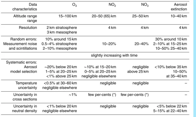
retrievals. The valid altitude range for the O₃measurements is roughly 15–100 km, for

20

NO2 20–50 km with the exception that when there is a high NO2load in the upper

at-mosphere, e.g., due to solar proton event, the valid altitude range extends up to 65 km. NO₃can be measured at 25–45 km and aerosols 10–40 km. In the GOMOS products also data at the other altitudes, outside the range considered to be valid, are given. If this data are used, it is recommended that, special attention to the data quality is taken.

25

(23)

ACPD

10, 6755–6796, 2010

J. Tamminen et.al

Title Page

Tables Figures

◭ ◮

Back Close

Full Screen / Esc

Interactive Discussion The GOMOS Level 1b and Level 2 data are freely available via ESA website

(http://http://eopi.esa.int/esa/esa?cmd=submission\&aoname=cat1) but registration is required. Instructions how to register and get GOMOS off-line data and GOMOS near real time data can be found at http://envisat.esa.int/handbooks/gomos/CNTR3. htm A comprehensive documentation for the GOMOS instrument including the data

5

disclaimer can be found at http://envisat.esa.int/handbooks/gomos/. The GOMOS Algorithm theorem basis document (ATBD) can be found at http://envisat.esa.int/ instruments/gomos/atbd/.

Acknowledgements. We thank European Space Agency for building the GOMOS instrument,

launching the ENVISAT satellite and for processing, archiving and distributing the GOMOS

10

data.

References

Bertaux, J. L., Hauchecorne, A., Dalaudier, F., Cot, C., Kyr öl ä, E., Fussen, D., Tamminen, J., Leppelmeier, G. W., Sofieva, V., Hassinen, S., d’Andon, O. F., Barrot, G., Mangin, A., Th éodore, B., Guirlet, M., Korablev, O., Snoeij, P., Koopman, R., and Fraisse, R.: First results

15

on GOMOS/Envisat, Adv. Space Res., 33, 1029–1035, 2004. 6757

Bertaux, J.-L., E., K., Fussen, D., Hauchecorne, A., Dalaudier, F., Sofieva, V., Tamminen, J., Vanhellemont, F., Fanton d’Andon, O., Barrot, G., Mangin, A., Blanot, L., Lebrun, J., Fehr, T., Saavedra, L., and Fraisse, R.: Global Ozone Monitoring by Occultation OF stars: an overview of GOMOS measurements on ENVISAT, Atmos Chem. Phys. Discuss., in review,

20

2010. 6757, 6758, 6771, 6772

Burrows, J. P., Richter, A., Dehn, A., Deters, B., s. Himmelmann, Voigt, S., and Orphal, J.: At-mospheric remote-sensing reference data from GOME – 2. temperature-dependent

absorp-tion cross secabsorp-tions of O₃ in the 231–794 nm range, J. Quant. Spectrosc. Radiat. Transfer,

61, 509–517, 1999. 6770

25

(24)

ACPD

10, 6755–6796, 2010

J. Tamminen et.al

Title Page

Tables Figures

◭ ◮

Back Close

Full Screen / Esc

Fussen, D., Vanhellemont, F., Bingen, C., Kyr öl ä, E., Tamminen, J., Sofieva, V., Hassinen, S., Sepp äl ä, A., Verronen, P., Bertaux, J.-L., Hauchecorne, A., Dalaudier, F., Renard, J.-B., Fraisse, R., Fanton d’Andon, O., Barrot, G., Mangin, A., Th éodore, B., Guirlet, M., Koopman, R., Snoeij, P., and Saavedra, L.: Global measurement of the mesospheric sodium layer by the star occultation instrument GOMOS, Geophys. Res. Lett., 31, L24110, doi:10.1029/

5

2004GL021618, 2004. 6771

Hauchecorne, A., Bertaux, J.-L., Dalaudier, F., Russell, J. M., Mlynczak, M. G., Kyr ¨ol ¨a, E., and

Fussen, D.: Large increase of NO₂in the north polar mesosphere in January-February 2004:

Evidence of a dynamical origin from GOMOS/ENVISAT and SABER/TIMED data, Geophys. Res. Lett., 34, 3810, doi:10.1029/2006GL027628, 2007. 6761

10

Hays, R. G. and Roble, P. B.: Stellar spectra and atmospheric composition, J. Atmos. Sci., 25, 1141–1153, 1968. 6757

Kyr ¨ol ¨a, E. and Tamminen, J.: GOMOS mission planning, in: ESAMS99, European Symposium on Atmospheric Measurements from Space, WPP-161, 101–110, ESA, Noordwijk, 1999. 6760

15

Kyr ¨ol ¨a, E., Tamminen, J., Leppelmeier, G. W., Sofieva, V., Hassinen, S., Bertaux, J.-L., Hauchecorne, A., Dalaudier, F., Cot, C., Korablev, O., d’Andon, O. F., Barrot, G., Mangin, A., Theodore, B., Guirlet, M., Etanchaud, F., Snoeij, P., Koopman, R., Saavedra, L., Fraisse, R., Fussen, D., and Vanhellemont, F.: GOMOS on Envisat: An overview, Adv. Space Res., 33, 1020–1028, 2004. 6757

20

Kyr ¨ol ¨a, E., Tamminen, J., Sofieva, V., Bertaux, J.-L., Hauchecorne, A., Dalaudier, F., Blanot, L., Fussen, D., Vanhellemont, F., d’Andon, O. F., Barrot, G., Mangin, A., Guirlet, M., Fehr, T., de Miguel, L. S., and Fraisse, R.: Retrieval of atmospheric parameters from GOMOS data, Atmos. Chem. Phys. Discuss. in review, 2010. 6758, 6763, 6764, 6765, 6766, 6767, 6768, 6769, 6772

25

Laine, M. and Tamminen, J.: Aerosol model selection and uncertainty modelling by adaptive MCMC technique, Atmos. Chem. Phys., 8, 7697–7707, 2008,

http://www.atmos-chem-phys.net/8/7697/2008/. 6769

Meijer, Y. J., Swart, D. P. J., Allaart, M., Andersen, S. B., Bodeker, G., Boyd, Braathena, G., Calisesia, Y., Claude, H., Dorokhov, V., von der Gathen, P., Gil, M., Godin-Beekmann, S.,

30

(25)

ACPD

10, 6755–6796, 2010

J. Tamminen et.al

Title Page

Tables Figures

◭ ◮

Back Close

Full Screen / Esc

ozone profiles using data from ground-based and balloon-sonde measurements, J. Geophys. Res., 109, D23305, doi:10.1029/2004JD004834, 2004. 6772

Press, W. H., Teukolsky, S. A., Vetterling, W. T., and Flannery, B. P.: Numerical Recipes in FORTRAN, The Art of Scientific Computing, Clarendon Press, Oxford, 1992. 6764

Rodgers, C. D.: Inverse Methods for Atmospheric sounding: Theory and Practice, World

Sci-5

entific, Singapore, 2000. 6758, 6772

Sepp ¨al ¨a, A., Verronen, P. T., Clilverd, M. A., Randall, C. E., Tamminen, J., Sofieva, V. F.,

Back-man, L., and Kyr ¨ol ¨a, E.: Arctic and Antarctic polar winter NO_xand energetic particle

precip-itation in 2002–2006, Geophys. Res. Lett., 34, L12810, doi:10.1029/2007GL029733, 2007. 6761

10

Sofieva, V., Tamminen, J., and Kyr ¨ol ¨a, E.: Modeling errors of GOMOS measurements: A sensitivity study, in: Atmosphere and Climate, Studies by Occultation Methods, edited by: Foelsche, U., Kirchengast, G., and Steiner, A., 67–78, Springer, 2006. 6767, 6771

Sofieva, V. F., Tamminen, J., Haario, H., Kyrl, E., and Lehtinen, M.: Ozone profile smoothness as a priori information in the inversion of limb measurements, Ann. Geophys., 22, 3411–

15

3420, 2004,

http://www.ann-geophys.net/22/3411/2004/. 6772, 6773

Sofieva, V. F., Kan, V., Dalaudier, F., Kyr ¨ol ¨a, E., Tamminen, J., Bertaux, J.-L., Hauchecorne, A., Fussen, D., and Vanhellemont, F.: Influence of scintillation on quality of ozone monitoring by GOMOS, Atmos. Chem. Phys., 9, 9197–9207, 2009,

20

http://www.atmos-chem-phys.net/9/9197/2009/. 6767, 6768

Tamminen, J.: Validation of nonlinear inverse algorithms with Markov chain Monte Carlo method, J. Geophys. Res., 109, D19303, doi:10.1029/2004JD004927, 2004. 6764, 6770 Tamminen, J. and Kyr ¨ol ¨a, E.: Bayesian solution for nonlinear and non-Gaussian inverse

prob-lems by Markov chain Monte Carlo method, J. Geophys. Res., 106, 14 377–14 390, 2001.

25

6764

Tamminen, J., Kyr ¨ol ¨a, E., and Sofieva, V.: Does prior information improve measurements?, in: Occultations for Probing Atmosphere and Climate - Science from the OPAC-1 Workshop, edited by: Kirchengast, G., Foelsche, U., and Steiner, A., 87–98, Springer Verlag, 2004. 6772

30

(26)

ACPD

10, 6755–6796, 2010

J. Tamminen et.al

Title Page

Tables Figures

◭ ◮

Back Close

Full Screen / Esc

Vervack, R. J., Yee, J., DeMajistre, R., and Swartz, W. H.: Intercomparison of MSX/UVISI-derived ozone and temperature profiles with ground-based, SAGE II, HALOE, and POAM III data, J. Geophys. Res., 108, 2–1, 2003. 6757

Yee, J.-H., Jr., R. J. V., Demajistre, R., Morgan, F., Carbary, J. F., Romick, G. J., Morrison, D., Lloyd, S. A., DeCola, P. L., Paxton, L. J., Anderson, D. E., Kumar, C. K., and Meng, C.-I.:

5

(27)

ACPD

10, 6755–6796, 2010

J. Tamminen et.al

Title Page

Tables Figures

◭ ◮

Back Close

Full Screen / Esc

Interactive Discussion Table 1.Occultation statistics during time period 2002–2008 divided by different stellar classes

depending on brightness and approximated surface temperature.

Bright Medium Dim Tot

Mv<0.8 Mv:0.8–2 Mv>2

Cool,T≤6000 K 3% 7% 22% 32%

T:6000–10 000 K 5% 4% 11% 19%

Hot,T≥10 000 K 11% 20% 18% 49%

(28)

ACPD

10, 6755–6796, 2010

J. Tamminen et.al

Title Page

Tables Figures

◭ ◮

Back Close

Full Screen / Esc

Interactive Discussion Table 2.Resolution of the GOMOS profile products.

Gas ≤30 km 30–40 km ≥40 km

O₃ 2 km 2–3 km 3 km

NO₂, NO₃ 4 km 4 km 4 km

(29)

ACPD

10, 6755–6796, 2010

J. Tamminen et.al

Title Page

Tables Figures

◭ ◮

Back Close

Full Screen / Esc

Interactive Discussion Table 3. GOMOS data characteristics and error contributions due to systematic and random

errors. The values correspond to the night time measurements. For NO₂ the higher altitude

limit corresponds to case with high NO₂concentration. (*) The impact of the systematic errors

due to the uncertainty in cross sections for NO₂and NO₃is only rough estimate.

Data O3 NO2 NO3 Aerosol

characteristics extinction

Altitude range 15–100 km 20–50 (65) km 25–50 km 10–40 km

range

Resolution 2 km stratosphere 4 km 4 km 4 km

3 km mesosphere

Random errors: 10% around 15 km 30% around 10 km

Measurement noise 0.5–4% stratosphere 10–20% 20–40% 2–10% at 15–25 km

and scintillations 2–10% mesosphere 10–50% 25–40 km

slightly increasing with time

Systematic errors:

Aerosol ∼20% below 20 km ∼10% at 15–20 km negligible <10% below 35 km

model selection 1–5% at 20–25 km 0–5% at 20–25 km above 25 km 10–50%

<1% above 25 km negligible elsewhere at 35–40 km

Temperature <0.5% at 30–60 km negligible negligible –

uncertainty negligible elsewhere

Uncertainty in ∼1% few per-cents (*) few per-cents (*) –

cross sections

Uncertainty in <1% below 20 km negligible negligible <5% below 22 km

(30)

ACPD

10, 6755–6796, 2010

J. Tamminen et.al

Title Page

Tables Figures

◭ ◮

Back Close

Full Screen / Esc

Interactive Discussion z

z

Earth radius

300 400 500 600 0

1 2 3 4x 104

300 400 500 600 0

1 2 3 4x 10

4

=> Transmission:

300 400 500 600 0

1

Signals: satellite orbit

(31)

ACPD

10, 6755–6796, 2010

J. Tamminen et.al

Title Page

Tables Figures

◭ ◮

Back Close

Full Screen / Esc

300 400 500 600

0 0.5 1

Transmission

Wavelength (nm)

STAR 3

300 400 500 600

0 0.5 1

Transmission

Wavelength (nm)

STAR 1

300 400 500 600

0 0.5 1

Transmission

Wavelength (nm)

STAR 117

300 400 500 600

0 0.5 1

Transmission

Wavelength (nm)

STAR 147

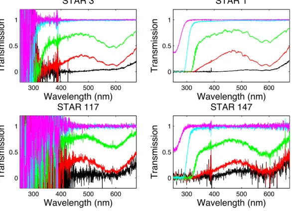
Fig. 2. Examples of GOMOS transmissions corrected for refractive effects measured using different stars, top row on left bright and cool star (M_v=−0.05,T=43 00 K) , on right bright and

hot star (M_v=−1.44,T=11 000 K) , bottom row on left dim and cool star (M_v=2.7, T=3800 K)

and on right dim and hot star (M_v=2.88, T=26 000 K). Five lines correspond to altitudes 10

(32)

ACPD

10, 6755–6796, 2010

J. Tamminen et.al

Title Page

Tables Figures

◭ ◮

Back Close

Full Screen / Esc

0 100 200 300 400

10 20 30 40 50 60 70 80 90 100

Signal−to−Noise ratio

Altitude (km)

S001: 250−350nm

S001: 420−550nm

S001: 550−675nm

S004: 250−350nm

S004: 420₋550nm

S004: 550₋675nm

S117: 250−350nm

S117: 420−550nm

S117: 550−675nm

Fig. 3.The average signal-to-noise ratio for three stars as a function of altitude in 2003. Star 1,

bright (M_v=−1.44) and hot star (T=11 000 K, solid line with circles) Star 4, bright and cool star

(M_v=−0.01,T=5800 K, solid line) and star 117, dim and cool star (M_v=2.7,T=3800 K, dashed

(33)

ACPD

10, 6755–6796, 2010

J. Tamminen et.al

Title Page

Tables Figures

◭ ◮

Back Close

Full Screen / Esc

Jan Feb Mar Apr May Jun Jul Aug Sep Oct Nov Dec

−80

−60

−40

−20 0 20 40 60 80

Latitude (deg)

(34)

ACPD

10, 6755–6796, 2010

J. Tamminen et.al

Title Page

Tables Figures

◭ ◮

Back Close

Full Screen / Esc

Interactive Discussion 9 12

−80

−60

−40

−20

0 20 40 60 80

2002

Latitude

100 200 300 400 500 600 700 800

3 6 9 12

2003

3 6 9 12

2004

3 6 9 12

2005

Month

3 6 9 12

2006

3 6 9 12

2007

3 6 9 12

2008

3 6 9 2009

Number of occultations

(35)

ACPD

10, 6755–6796, 2010

J. Tamminen et.al

Title Page

Tables Figures

◭ ◮

Back Close

Full Screen / Esc

Longitude (deg)

Latitude (deg)

GOMOS lowest altitude, 30 brightest stars 2003−06

−150 −100 −50 0 50 100 150

−80

−60

−40

−20

0 20 40 60 80

5 6 7 8 9 10 11 12 13 14 15 16 17 18 19

Stopping altitude (km)

(36)

ACPD

10, 6755–6796, 2010

J. Tamminen et.al

Title Page

Tables Figures

◭ ◮

Back Close

Full Screen / Esc

−1 −0.8 −0.6 −0.4 −0.2 0 0.2 0.4 0.6 0.8 1

25 30 35 40 45 50 55 60 65 70

Correlation coefficient

Altitude (km)

Correlation with ozone error estimate

no2 no3 a1 a2 a3

Fig. 7. Examples of correlation coefficients between the error estimates of horizontally

inte-grated O₃and NO₂(solid blue line), NO₃(green circles) and three aerosol parameters (dashed

(37)

ACPD

10, 6755–6796, 2010

J. Tamminen et.al

Title Page

Tables Figures

◭ ◮

Back Close

Full Screen / Esc

−0.5 0 0.5 1

20 25 30 35 40 45 50 55 60

Correlation coefficient

Altitude (km)

Corrlation between layers

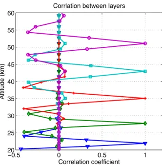
Fig. 8. Correlation of the retrieval error with neighbouring layers. Five selected altitudes (23,

(38)

ACPD

10, 6755–6796, 2010

J. Tamminen et.al

Title Page Abstract Introduction Conclusions References Tables Figures ◭ ◮ ◭ ◮ Back Close

Full Screen / Esc

0 5

x 1012

10 15 20 25 30 35 40 Altitude (km)

O3 median values

0 1 2 3

x 109

10 15 20 25 30 35 40

Number density (1/cm3) NO2 median values

0.5 1 1.5 2

x 107

10 15 20 25 30 35 40

NO3 median values

0 2 4 6

x 10−4

10 15 20 25 30 35 40

Aerosol median values

A−1

A−2

A−3

A−4

A−5 A−6 A−7

−40 −20 0 20 10 15 20 25 30 35 40 Altitude (km)

O3 relative difference

A−1

A−2

A−4

A−5

A−6

A−7

−40−20 0 20 40

10 15 20 25 30 35 40

Relative difference (%)

Altitude (km)

NO2 relative difference

−10100 0 100 15 20 25 30 35 40 Altitude (km)

NO3 relative difference

−50−25 0 25 50

10 15 20 25 30 35 40 Altitude (km)

Aerosol relative difference

33

(39)

ACPD

10, 6755–6796, 2010

J. Tamminen et.al

Title Page

Tables Figures

◭ ◮

Back Close

Full Screen / Esc

1 2 3

20 30 40 50 60 70 80 90 100 110

B.!G.spread (km)

Altitude (km)

Vertical R03057/S018) Typical (R03057/S002) Oblique (R03057/S001)

1 2 3

20 30 40 50 60 70 80 90 100 110

B.!G.spread (km)

Altitude (km)

Vertical R03057/S018) Typical (R03057/S002) Oblique (R03057/S001)