Technical Note: Feasibility of CO<sub>2</sub> profile retrieval from limb viewing solar occultation made by the ACE-FTS instrument

(1)

ACPD

9, 411–462, 2009

Feasibility of CO₂ profile retrieval from

ACE-FTS

P. Y. Foucher et al.

Title Page

Abstract Introduction

Conclusions References

Tables Figures

◭ ◮

Back Close

Full Screen / Esc

Printer-friendly Version

Interactive Discussion

Atmos. Chem. Phys. Discuss., 9, 411–462, 2009 www.atmos-chem-phys-discuss.net/9/411/2009/ © Author(s) 2009. This work is distributed under the Creative Commons Attribution 3.0 License.

Atmospheric Chemistry and Physics Discussions

This discussion paper is/has been under review for the journalAtmospheric Chemistry

and Physics (ACP). Please refer to the corresponding final paper inACPif available.

Technical Note: Feasibility of CO

₂

profile

retrieval from limb viewing solar

occultation made by the ACE-FTS

instrument

P. Y. Foucher1, A. Ch ´edin1, G. Dufour2, V. Capelle1, C. D. Boone3, and P. Bernath3,4

1

Laboratoire de M ´et ´eorologie Dynamique/Institut Pierre Simon Laplace, Ecole Polytechnique, 91128 Palaiseau, France

2

Laboratoire Inter-universitaire des Syst èmes Atmosph ériques, Facult é des Sciences et Technologies, 61 avenue du G én éral de Gaulle, 94010 Cr éteil, France

3

Department of Chemistry, University of Waterloo, Ontario, N2L3G1, Canada 4

Department of Chemistry, University of York, Heslington, York, UK.YO105DD, UK

Received: 29 September 2008 – Accepted: 15 October 2008 – Published: 7 January 2009

Correspondence to: P. Y. Foucher (pierre-yves.foucher@lmd.polytechnique.fr)

(2)

ACPD

9, 411–462, 2009

ACE-FTS

Title Page

Tables Figures

◭ ◮

Back Close

Full Screen / Esc

Abstract

Major limitations of our present knowledge of the global distribution of CO2 in the

at-mosphere are the uncertainty in atmospheric transport mixing and the sparseness of in situ concentration measurements. Limb viewing space-borne sounders, observing the atmosphere along tangential optical paths, offer a vertical resolution of a few kilo-5

metres for profiles, which is much better than currently flying or planned nadir sounding instruments can achieve. In this paper, we analyse the feasibility of obtaining CO₂ ver-tical profiles in the 5–25 km altitude range from the Atmospheric Chemistry Experiment Fourier Transform Spectrometer (ACE-FTS, launched in August 2003), high spectral

resolution solar occultation measurements. Two main difficulties must be overcome: (i)

10

the accurate determination of the instrument pointing parameters (tangent heights) and

pressure/temperature profiles independently from an a priori CO2 profile, and (ii) the

potential impact of uncertainties in the temperature knowledge on the retrieved CO2

profile. The first di_fficulty has been solved using the N₂ collision-induced continuum

absorption near 4µm to determine tangent heights, pressure and temperature from

15

the ACE-FTS spectra. The second difficulty has been solved by a careful selection of

CO₂ spectral micro-windows. Retrievals using synthetic spectra made under realistic

simulation conditions show a vertical resolution close to 2.5 km and accuracy of the or-der of 2 ppm after averaging over 25 profiles. These results open the way to promising studies of transport mechanisms and carbon fluxes from the ACE-FTS measurements. 20

1 Introduction

Determining the spatial and temporal structure of surface carbon fluxes has become a major scientific issue during the last decade. In the so-called “inverse” approach, observed atmospheric concentration gradients are used to disentangle surface fluxes, given some description of atmospheric transport. This approach has been widely used 25

(3)

esti-ACPD

9, 411–462, 2009

ACE-FTS

Title Page

Tables Figures

◭ ◮

Back Close

Full Screen / Esc

mate the spatial distribution of annual mean surface fluxes (Gurney, 2002) and their interannual variability (Baker, 2006). Major limitations of the inverse approach are the

uncertainties in atmospheric transport and the sparseness of atmospheric CO2

con-centration measurements based on a network of about 100 surface stations unevenly

distributed over the world. As a consequence, the number of CO2 in situ

observa-5

tions, particularly from aircraft (research campaigns or regular aircraft measurements: see, e.g., Andrew (2001); Brenninkmeijer (1999); Matsueda (2002); Engel (2006) and references herein), has increased in recent years.

Although sporadic in time and space, in situ aircraft measurements are useful to test the modeling of the transport of air from the surface to the upper troposphere 10

and lower stratosphere as well as the incursion of stratospheric air back into the

up-per troposphere. Since CO2 is inert in the lower atmosphere, its long-term trend and

pronounced seasonal cycle (due to the uptake and release by vegetation) propagate

from the surface, and the di_fference between atmospheric and surface mixing ratios

is determined by the processes that transport surface air throughout the atmosphere, 15

including advection, convection and eddy mixing (Shia, 2006). Tropospheric air enters the stratosphere predominantly in the tropics where air is lifted upwards and pole-wards on timescales of several years as part of the Brewer-Dobson circulation (Holton,

1995). In the extra-tropics of the upper troposphere during winter, the CO2

concentra-tion is particularly influenced by the air descending from the lower stratosphere in the 20

downward branch of the Brewer-Dobson circulation. Because it takes several months to transport surface air to the lower stratosphere, the CO2mixing ratio is lower and the

seasonal cycle is di_fferent there as compared to the troposphere (Plumb, 1992, 1996;

Shia, 2006).

Engel (2006) show that there is very little CO2 variability throughout the lower most

25

stratosphere (LMS) in autumn. During winter and spring, the CO₂ values in the LMS

are mostly below the tropospheric values. On the contrary, during summer, CO2 is

higher in the stratosphere than in the troposphere. This particular behaviour of CO2

(4)

lower-ACPD

9, 411–462, 2009

ACE-FTS

Title Page

Tables Figures

◭ ◮

Back Close

Full Screen / Esc

most stratosphere with elevated CO₂was caused by relatively fast transport from the

upper tropical troposphere, where tropospheric summertime CO2 values are higher

than in mid latitudes during the same period. However, the transport processes, and in particular small-scale dynamical processes, such as convection and turbulence as-sociated with frontal activity, which cannot be explicitly resolved by chemistry-transport 5

models in this region, are complex and our understanding is still poor. B ¨onisch (2008) evaluated transport in three-dimensional chemical transport models in the upper

tropo-sphere and lower stratotropo-sphere by using observed distributions of CO2and SF6. They

show that although all models are able to capture the general features in tracer

dis-tributions including the vertical and horizontal propagation of the CO₂seasonal cycle,

10

important problems remain such as: (i) a too strong Brewer-Dobson circulation caus-ing an overestimate of the tracer concentration in the LMS durcaus-ing winter and sprcaus-ing, (ii) a too strong tropical isolation leading to an underestimate of the tracers in the LMS during winter. Moreover, all models tested su_ffer to some extent from di_ffusion and/or too strong mixing across the tropopause. In addition, the models show too weak verti-15

cal upward transport into the upper troposphere during the boreal summer.

In recent years it has become possible to measure atmospheric CO₂ from space.

Satellite-based observations by the nadir-viewing vertical sounders TIROS-N Opera-tional Vertical Sounder (TOVS), Atmospheric Infrared Sounder (AIRS) (Ch ´edin, 2002, 2003a,b; Crevoisier, 2004; Engelen, 2005), or SCIAMACHY (Buchwitz, 2005), and now 20

the Infrared Atmospheric Sounder Interferometer (IASI) have the potential to

dramati-cally increase the spatial and temporal coverage of CO2measurements. In the near

fu-ture (early 2009), the Orbiting Carbon Observatory (OCO) and the Greenhouse gases

Observing Satellite (GOSAT) missions will be launched to measure CO2(and methane,

for GOSAT) column densities from orbit. The satellite data products are all vertically 25

integrated concentrations rather than the profile measurements that are essential to

a comprehensive understanding of distribution mechanisms of CO2. The difference

between the column-averaged CO2mixing ratio and the surface value varies from 2 to

(5)

ACPD

9, 411–462, 2009

ACE-FTS

Title Page

Tables Figures

◭ ◮

Back Close

Full Screen / Esc

can contribute significantly to this difference because this portion of the column

consti-tutes approximately 20% of the column air mass and the CO₂mixing ratios in this

re-gion can differ by 5 ppmv or more from the CO2mixing ratios at the surface (Anderson, 1996; Matsueda, 2002; Shia, 2006). With limb sounders that observe the atmosphere along tangential optical paths, the vertical resolution of the measured vertical profiles is 5

of the order of a few kilometers, much better than can be achieved with nadir sounding instruments. The Atmospheric Chemistry Experiment Fourier Transform Spectrometer (ACE-FTS), launched in August 2003, is a limb sounder that records solar occultation measurements (up to 30 occultations each day) with coverage between approximately 85◦

N and 85◦

S (Bernath, 2005), with more observations at high latitudes than over the 10

tropics (Bernath, 2006). The ACE-FTS has high spectral resolution (0.02 cm−1

) and the signal-to-noise ratio of ACE-FTS spectra is higher than 300:1 over a large portion

(1000–3000 cm−1

) of the spectral range covered (750–4400 cm−1

). Our analysis is

or-ganised as follows. We first present the method used to retrieve CO₂profiles from limb

viewing observations, the problems encountered in estimating the tangent heights of 15

the measurements and the strategy adopted using the N2continuum absorption. We

then discuss in detail the crucial step of selecting appropriate spectral regions to use in the retrievals (the so-called “micro-windows”). The micro-windows are optimized to pro-vide the maximum amount of information on the target variables: instrument pointing

parameters and CO₂profiles. The selection procedure takes into account errors due to

20

instrumental and spectroscopic parameters noise, to interfering species (species other

than CO2) and to temperature uncertainties. Constraints on the estimator are then

discussed in detail and results are presented on the degrees of freedom, the vertical resolution, the error and standard deviation of the retrieved profiles. Finally, synthetic results are presented and discussed.

(6)

ACPD

9, 411–462, 2009

ACE-FTS

Title Page

Tables Figures

◭ ◮

Back Close

Full Screen / Esc

2 Retrieving CO₂profiles from limb viewing observations: problems and

strategy

2.1 Instrument pointing

Interpreting limb viewing observations in terms of atmospheric variables requires accurate knowledge of instrument pointing parameters (tangent heights) and pres-5

sure/temperature (hereafter referred to as “pT”) vertical profiles. Temperature and tangent heights can be viewed as independent parameters whereas pressure can be calculated from temperature and altitude by using the hydrostatic equilibrium equa-tion. Reactive trace gases are the usual target species of limb-viewing instruments, so pointing parameters are simultaneously retrieved with pT by the analysis of properly 10

selected CO₂ lines under the assumption (questionable, in certain cases) of a weak

variation of its atmospheric concentration around a given a priori value. In the

strato-sphere, pT and tangent height errors caused by a variation of the CO2 mixing ratio

is not the major source of error, and, for example, is about 10% of the total error

as estimated for the MIPAS sounder for a CO₂ uncertainty of 3 ppm (von Clarmann,

15

2003). This approach becomes more problematic in the troposphere because: (i) the

weak CO2 lines used are more sensitive to an error in the assumed CO2

concentra-tion (Park, 1997), and (ii) the variability in this concentraconcentra-tion is much larger than in the

stratosphere. Moreover, when the target gas is CO2 itself, determining the pointing

parameters from CO2 lines is clearly impossible and would obviously introduce

arti-20

ficial correlations between the pointing and the CO₂ concentration. A critical step in

this research has therefore been to develop a method of obtaining pT profiles and

tan-gent heights independent of any a priori CO2knowledge. Only absorbing gases whose

abundance is well known and constant can be used to achieve this goal.

In the case of ACE v2.2 retrieval (Boone, 2005), pT and tangent heights are fitted 25

simultaneously using suitable CO2 lines above 12 km; below 12 km, pT profiles are

from the Canadian Meteorological Centre (CMC) analyses data, and tangent heights

are fitted using CO2 lines around 2600 cm

−₁

(7)

ACPD

9, 411–462, 2009

ACE-FTS

Title Page

Tables Figures

◭ ◮

Back Close

Full Screen / Esc

ACE v2.2 retrieval are more sensitive to pointing parameters than to the CO₂ volume

mixing ratio; however below 12 km the CO₂lines around 2600 cm−₁

are very sensitive

to the CO2concentration and the bias on the tangent heights due to the assumed CO2

concentration increases dramatically. To determine tangent heights and pT profiles

from ACE-FTS spectra that are independent of CO₂, we make use of the N₂absorption

5

continuum (Lafferty, 1996). The possibility of employing the N2continuum in retrievals was mentioned in Boone (2005), but this paper represents the first time such a retrieval strategy has been implemented.

2.2 Retrieval strategy

The retrieval process has two main steps: pointing parameter estimation and then CO2

10

vertical profile estimation. These retrievals both use a similar least-squares retrieval method. The target variable is a vector containing tangent heights and a temperature profile in the first step or a CO2profile in the second step. The method described below uses a CO2profile as the target variable but there is no significant change in the case of a pointing parameter retrieval. ACE-FTS measurements can be interpreted in terms of 15

CO2profiles using a least-squares retrieval method based on optimal estimation theory

(Gelb, 1974; Rodgers, 2000) and a non linear iterative estimator which minimizes the cost function:

χ_i2₌ y_obs−y(xi)TS−1

e yobs−y(xi)

+ xi −x_aTR xi −x_a (1)

wherey_obs is the measurement vector and y(xi) the related computed forward model

20

vector for the iterative stepi,xi is the target CO2profile andxaits a priori value. Seis

the random noise error covariance matrix. In order to take non linearity into account, the following iterative process, from one state of the target profile to the next, is used (Levenberg, 1944; Marquardt, 1963):

xi+1−xi = KTS−1

e K+R+λD

−₁

KTS−1

e yobs−y(xi)

−R xi −x_a (2)

(8)

ACPD

9, 411–462, 2009

ACE-FTS

Title Page

Tables Figures

◭ ◮

Back Close

Full Screen / Esc

whereKis then×mJacobian matrix containing the partial derivatives of allnsimulated measurements y(x) with respect to allm unknown variables x : K(u, l)₌∂y_∂(_xx₍)(_l₎u) with (u, l) ∈ [1, n][1, m], and R is a regularization matrix. The term D controls the “rate of descent” of the cost function in the least-square process. The scalar increases when the cost function is not reduced in a given iteration and decreases when the cost 5

function decreases. Here the matrix D is assumed diagonal and takes into account

the possibility that the expected variance of each element of the state vector may be di_fferent:

D=diag KTS−1

e K+R

(3)

The regularization matrixRcan take various forms, the simplest being a diagonal

ma-10

trix containing the a priori inverse variance (if known) of the target variable. When the target variable covariance is known, one of the best choices (Rodgers, 2000) is the inverse a priori covariance matrix S−1

a . However, when little information is

avail-able, a common choice is the use of a Tikhonov regularization (Tikhonov, 1963) with

a squared and scaled finite difference smoothing operator (Twomey, 1963; Phillips,

15

1962; Steck, 2002). (see Sects. 3.2 and 4 for more details).

2.3 4A/OP-limb radiative transfer model

The forward solution of the radiative transfer equation is provided by the 4A/OP-limb Radiative Transfer Model (RTM). 4A (for Automatized Atmospheric Absorption Atlas) is a fast and accurate line-by-line radiative transfer model (Scott, 1981) de-20

veloped and maintained at Laboratoire de M ´et ´eorologie Dynamique (LMD; see http: //ara.lmd.polytechnique.fr) and was made operational (OP) in cooperation with the French company Noveltis (see http://www.noveltis.net/4AOP for a description of the 4A/OP version). 4A allows fast computation of the transmittance of discrete atmo-spheric layers (the nominal spectral resolution is 5×10−4cm−1but can be changed by 25

(9)

ACPD

9, 411–462, 2009

ACE-FTS

Title Page

Tables Figures

◭ ◮

Back Close

Full Screen / Esc

atmospheric molecular species. The atlases were created by using the line-by-line and layer-by-layer model, STRANSAC (Scott, 1974), in its latest 2000 version with up-to-date spectroscopy from the GEISA spectral line data catalog (Jacquinet-Husson,

2008). The 4A/OP-limb RTM also includes continua of N2, O2and H2O. For the present

application, 4A/OP-limb uses new atlases suitable for a 1 km atmospheric grid spacing 5

for the altitude range surface-100 km (100 levels). This 1 km discretization is used here for pressure, temperature and gas concentration profiles, as well as for the Jacobian calculations.

3 Spectral micro-window selection

3.1 Spectral micro-windows pre selection: a sensitivity analysis

10

To be selected and finally included in the measurement vector, a spectral micro-window must satisfy the obvious criteria of high sensitivity to the target variables (here the pointing parameters or CO₂) and low sensitivity to non target variables. Investigations have to be carried out to analyze the quality of the spectral fit in order to minimize systematic contributions to the final error budget.

15

3.1.1 Pointing parameters and the N2continuum absorption

As explained in Sect. 2, micro-windows are selected in the N₂ collision-induced

ab-sorption continuum near 4.0 µm to fit tangent heights and pT profiles in the 5–25 km altitude range. N2continuum absorption is significant for large optical paths obtained in

the limb viewing geometry. 4A/OP-limb RTM uses an empirical model (Lafferty, 1996)

20

determined from experimental data, which includes N2–N2 and N2–O2 collisions and

covers the 190–300 K temperature range. Measurements cover the range 2125 cm−1

(4.7 µm) to 2600 cm−1

(3.8 µm) with a spectral resolution of 0.25 cm−1

. N₂ continuum

(10)

ACPD

9, 411–462, 2009

ACE-FTS

Title Page

Tables Figures

◭ ◮

Back Close

Full Screen / Esc

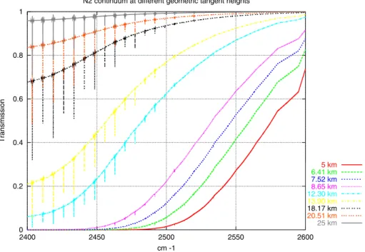
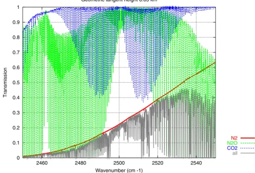
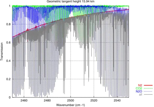
saturated below 5 km; the atmospheric transmittance dynamic range is large in the 5– 25 km altitude range as seen in Fig. 1. This spectral region also contains absorption

from N2O and CO2lines. The far wing contributions from these molecules, which are

difficult to model, may affect the baseline level in the vicinity of the N2continuum (see

Figs. 2 and 3), thereby complicating the analysis. For wavenumbers below 2385 cm−1

5

the spectrum is saturated up to 25 km due to CO₂ far wing absorption and the e_ffect

of this contribution on the N2baseline remains significant up to 2500 cm

−₁

for the

low-est altitudes and up to 2450 cm−1

at 20 km. The contribution from N2O line wings is

important for the lowest altitudes from 2400 cm−1

to 2495 cm−1

and from 2515 cm−1

to 2600 cm−1

but the N₂O and CO₂ impact on the baseline rapidly decreases with

in-10

creasing tangent height (see Fig. 3 for a geometric tangent height of 15.9 km). Figure 2 shows that at 8.65 km geometric tangent height (corresponding to a true tangent height around 7.7 km), CO₂and N₂O contributions to the N₂absorption are only negligible in

a small spectral region around 2500 cm−1, whereas at 15.90 km, Fig. 3 shows that

a larger spectral region, from 2480 to 2520 cm−1

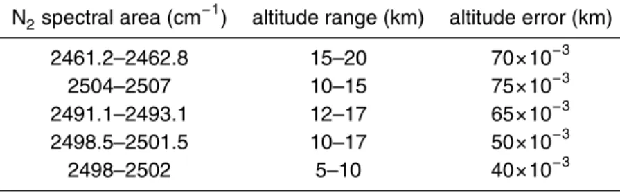
, is available. In summary, the spec-15

tral ranges employed for pointing parameter retrieval using the N₂ continuum are as

follows: 2495–2505 cm−1

in the 5–10 km altitude range, 2490–2520 cm−1

in the 10–

15 km altitude range, 2480–2505 cm−1and around 2461 cm−1in the 15–25 km altitude

range.

The pure N₂ collision-induced absorption temperature dependence varies with

20

wavenumber (Lafferty, 1996). Below 2450 cm−1, the absorption coefficient decreases

with temperature, while the reverse is true for wavenumbers above 2450 cm−1

; however the sensitivity to variations in tangent height is relatively constant throughout the con-tinuum. To retrieve temperature and tangent height simultaneously above 12 km (see

Part 2.1), it is necessary to choose at least two different N2 spectral micro-windows

25

having different sensitivities to temperature, i.e., micro-windows around 2450 cm−1 (or

below) and micro-windows around 2500 cm−1

. However, in the 2450 cm−1

spectral

(11)

ACPD

9, 411–462, 2009

ACE-FTS

Title Page

Tables Figures

◭ ◮

Back Close

Full Screen / Esc

far wings. In this paper we therefore focus mainly on tangent height retrievals although the results of a simultaneous fit are presented in Part 5.

3.1.2 CO₂concentrations: an analysis of CO₂lines sensitivity

The selection of CO2spectral micro-windows for both concentration and temperature

retrievals is based on the analysis of 4A/OP-limb RTM simulated transmittances and 5

Jacobians. In a first step, CO2 lines with concentration Jacobians peaking within the

tangent altitude range considered are selected. In a second step, CO2lines overlapped

by other species are rejected on the basis of the relative importance of the CO2

Jaco-bian and the JacoJaco-bians of the other species. In a third step, only the CO₂ lines with

a small lower state energyE” are selected to minimize the line intensity dependence

10

on temperature. In fact, it may be shown that for a micro-window corresponding to a CO₂line with a low value of the lower state energyE”, there exists a tangent height at which the temperature Jacobian is almost equal to zero (Park, 1997) and the sign of the temperature Jacobian is positive above this critical altitude and negative below. Finally, spectral regions for which radiative transfer model is not relevant are rejected. 15

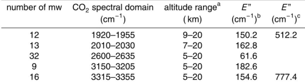
Altogether, about 80 CO2micro-windows were pre-selected from five different

spec-tral domains as shown in Table 1 (column 1: number of micro-windows; column 2: spectral domain). In this table they are classified according to the altitude range in

which they are suitable for determining the CO2 profile (column 3). Column 4 gives

the average value ofE” for the lines selected in each spectral domain. These values

20

are much smaller than those corresponding to micro-windows traditionally selected for

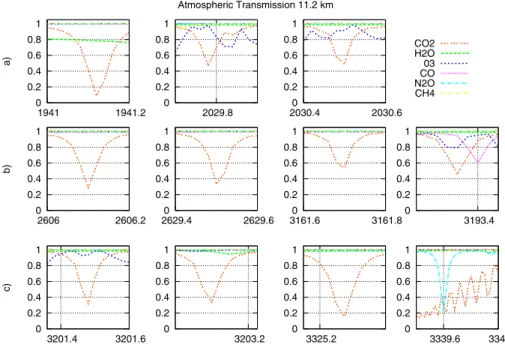
temperature retrieval when the target variable is not CO2 (see column 5). Figures 4

and 5 show examples of pre-selected CO2micro-windows transmittances (Fig. 4) and

sensitivities (Fig. 5), for each contributing species, versus wavenumber at a tangent height of 11.2 km. In Fig. 4, different situations are seen: (i) relatively clean CO2 win-25

dows (b1, b2, b3, c2 and c3); (ii) windows with modest contributions from other species

(O₃in a3 and c1); windows with more pronounced signatures from other species (H₂O

(12)

ACPD

9, 411–462, 2009

ACE-FTS

Title Page

Tables Figures

◭ ◮

Back Close

Full Screen / Esc

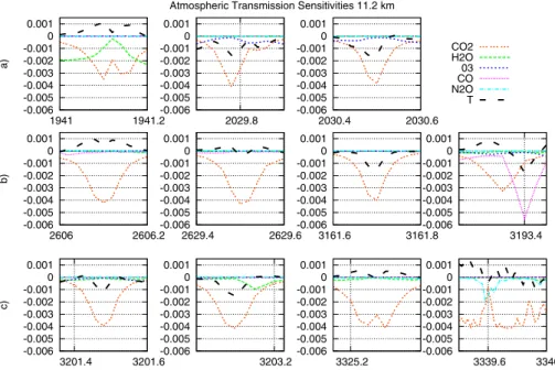
has also been tested (although no results are presented here). The impact of species is confirmed by Fig. 5 which shows transmittance Jacobians for the same species and

for the same CO2 micro-windows. In this figure the temperature Jacobians are also

plotted (black dashed line) which display different behaviours: positive sensitivity for a1, b1, and c3; negative sensitivity for a2, a3, b3, c1 and c2; sensitivity changing sign 5

within the spectral interval for b4 and c4. Almost zero sensitivity is observed for b2.

The expected presence of opposite temperature Jacobian signs, between 2030 cm−1

and 2606 cm−1

for example, is a very interesting point. Indeed, if two CO₂ lines with

opposite temperature Jacobians for the same altitude range are used for CO2retrieval,

the impact of temperature uncertainties on the retrieval in this altitude range is reduced 10

(see part 3.2 on micro-windows optimization). When a micro-window is nearly free of absorption by other species, an easy method to select (or reject) the micro-window is to look at the ratio between its sensitivity to temperature to its sensitivity to CO2. The presence of an interfering species may be seen as a problem in terms of the error bud-get. However, this interference can lead to the temperature sensitivity changing sign 15

within the micro-window (as in b4, for example) which may result in a less significant temperature sensitivity than for a cleaner micro-window with a more uniform (positive or negative) temperature sensitivity.

The instrumental noise, as well as the ability of the RTM to properly model the trans-mittance, also plays an important role in the micro-window selection process: a “good” 20

micro-window in term of sensitivity can be useless if the measurement or model errors are too large. Selecting an optimal set of micro-windows well distributed in the 5–25 km altitude range requires a detailed analysis of the retrieval error budget.

3.2 Optimization of the micro-windows selection: error budget analysis

The total error budget on the target variablex,errX(l), at altitude levell, essentially 25

results from the instrumental noise propagation error, error from parameter uncertain-ties (the effect of pT profiles and tangent height errors on CO2retrievals, for example),

(13)

de-ACPD

9, 411–462, 2009

ACE-FTS

Title Page

Tables Figures

◭ ◮

Back Close

Full Screen / Esc

pends on the quality of the micro-window selection. Following von Clarmann (1998) and Dudhia (2002), the pre-selected micro-windows have been optimized by adjusting their boundaries and numbers so that the total retrieval error is minimized.

errX(l)=

v u u u t

 σ(l)+

p

X

j

ej₍_l₎2



 (4)

ej ₌(KTSe−1

K+R)−₁

×KTSe−1K_j∆_j (5)

5

S_n =(KTSe−1

K+R)−₁

×KTSe−1K×(KTSe−1K+R)−1 (6)

σ₌diag(S_n) (7)

The total error budget errX(l) on the target variable is defined for altitude level l

by Eq. (4) whereσ(l) (Eq. 7) is the diagonal element of the random error propagation

covariance matrixS_n(Eq. 6),pis the number of non target parameters,ej(l) (Eq. 5) is 10

the error due to parameterjat levell, withK_j the partial derivative of the corresponding

transmittance matrix and∆j the standard deviation vector of parameterj uncertainties.

Micro-window optimization requires the use of a regularization matrix, especially for CO₂. Discussion of this constraint in terms of accuracy and vertical resolution is

pre-sented in Part 4. In short, to optimize micro-windows, a first order finite difference

15

Tikhonov regularization (see Sect. 2) is used to optimize temperature and tangent height micro-windows and a covariance matrix from the MOZART 3-D chemical

trans-port model (Horowitz, 2003) is used to optimize CO2 micro-windows. Note that the

regularization does not modify the micro-window selection but is necessary to evaluate the total error budget.

20

3.2.1 Optimized N2continuum micro-windows

(14)

ACPD

9, 411–462, 2009

ACE-FTS

Title Page

Tables Figures

◭ ◮

Back Close

Full Screen / Esc

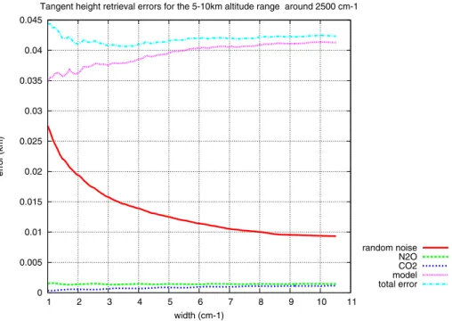
absorption and the retrieval error in general. Starting from a minimal width of 1 cm−1

for an optimized micro-window, the total retrieval error is estimated as a function of the increasing width of the window. The random noise error, errors due to 5%

per-cent changes in CO2and N2O concentrations, and model errors due to CO2and N2O

far wing contributions and N2continuum, estimated on the basis of comparisons with

5

ACE-FTS measurements and experimental measurements (La_fferty, 1996), are taken

into account in this analysis. The random noise variance used here is taken as twice the instrument noise variance to account for random errors from computation. Fig-ure 6 shows the variation of the total error and of error components (random noise, CO2, N2O, model) as a function of the width of the micro-window for the spectral range 10

around 2500 cm−1

. These errors have been averaged for tangent heights between 5 and 10 km. The initial micro-window width is 1 cm−1

(50 spectral points) and its central

wavenumber is 2500.7 cm−1, which corresponds to the centre of the CO2 band (see

Figs. 2 and 3). Then, step by step, 2 symmetric spectral points are added and the

tangent height retrieval error is again estimated. From 1 cm−1

to 9 cm−1

width, the 15

noise propagation error decreases from 25 m to 9 m, the model error increases from

35 m to 42 m, the error due to uncertainties in CO2 and N2O remains less than 5 m.

The total error reaches its minimum value (about 40 m) at 3.5 cm−1

width and remains approximately constant for larger widths. Similar results are obtained for the same spectral range for the 10–15 km altitude range (not shown). The total error comes to 20

about 50 m; model error significantly increases with the width (due to N2O and CO2

far wing error model as the N₂continuum model error is quite constant in this spectral

region); retrieval errors due to N2O and CO2 concentration uncertainties remain low

(less than 5 m). For this altitude range, in the spectral interval 2495–2505 cm−1

, the

optimal micro-window width is 3 cm−1

. Results for the same altitude range in other 25

spectral intervals, 2490–2495 cm−₁

and 2505–2520 cm−₁

(15)

ACPD

9, 411–462, 2009

ACE-FTS

Title Page

Tables Figures

◭ ◮

Back Close

Full Screen / Esc

3.2.2 Optimized set of CO₂lines micro windows

In the case of CO2, many micro-windows may be considered for retrieving its

con-centration at a given altitude. Optimization of the set of pre-selected micro-windows is based on the evaluation of component and total errors due to noise propagation, temperature uncertainties, and, eventually, interfering species. The random noise in-5

troduced accounts for instrumental noise and CO₂ random spectroscopic parameters

error. Resulting from comparisons between observations and model simulations, the

transmittance model random error for CO2 has been taken equal to 0.5×10

−2 (i.e.: twice larger than instrumental random noise in the center of the band). Micro-windows selection follows two main steps: (i) optimization of the width of each micro-window, 10

(ii) creation of an optimum set of micro-windows.

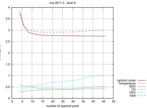
For each pre-selected micro-window we first evaluate the impact of its spectral width

on the retrieval error. Figure 7a shows, for a micro-window around 2611.3 cm−1and for

a geometric altitude of 6 km, the retrieval errors as a function of width. Noise propaga-tion error decreases from 3.7 to 2.7 ppm when the size of the micro-window increases 15

but errors due to interfering species and to temperature increase and become non

neg-ligible. N2O and temperature errors are around 0.5 ppm whereas H2O error increases

from 0.4 to 1 ppm. The optimum size (minimum of total error) corresponds to 14 spec-tral points (0.28 cm−₁

). In fact, the optimal size depends on the tangent altitude: for

the same micro-window, but at 16 km, the character of the error budget is different:

20

H2O and N2O errors are negligible and temperature error increases (see Fig. 7b). In

this case, the minimum of the total error is reached for a width of about 10 spectral points (0.2 cm−1). The micro-window at 2604.6 cm−1 at 6 km altitude (Fig. 7c) illus-trates the example of a poor micro-window: the total error increases with the width of the micro-window. Temperature error increases from 2 to 4.5 ppm, random noise error 25

decreases from 3.5 to 2.5 ppm, and N2O and H2O errors increase up to 1 ppm; the

(16)

ACPD

9, 411–462, 2009

ACE-FTS

Title Page

Tables Figures

◭ ◮

Back Close

Full Screen / Esc

at 1934.8 cm−1

with an optimal size corresponding to 30 spectral points (0.6 cm−1

); however, one can see that the temperature error first increases and then decreases:

this is mostly due to the presence of H₂O absorption which modifies the sensitivity to

temperature and may even change the sign of the temperature Jacobian. Figure 7e shows, for the same altitude, a poor micro-window due to a significant contribution of 5

H₂O to the error. Finally, for each altitude, pre-selected width-optimized micro-windows are ranked according to their total error.

The second step of the optimization procedure consists of starting from a first “best set” of 5 micro-windows chosen among the micro-windows with lowest total error and well distributed within the 5–25 km altitude range. From this first set, the number of 10

micro-windows is progressively increased by adding windows of good quality (total error) while observing their impact on the total error.

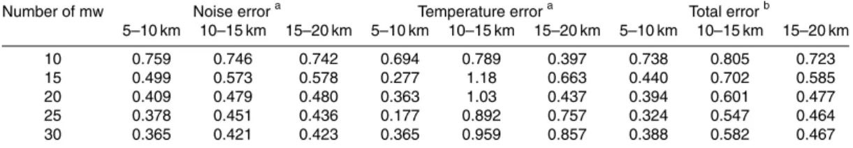
Table 3 gives, for five augmented sets of micro-windows (column 1), the ratio be-tween the corresponding total error and that obtained with the original 5-micro-window set. Regarding the random noise error (columns 2–4), the retrieval error decreases 15

when the number of micro-windows increases at each altitude range. A limit is reached for the set with 30 micro-windows. Temperature error (columns 5–7) behaviour varies with the altitude range: (i) in the 5–10 km altitude range the error decreases up to the 15 micro-windows set and then fluctuates with a minimum for the 25 micro-windows set, this being due to the fact that, for this altitude range, the temperature sensitivity sign 20

frequently changes from one micro-window to another, leading to error compensation; (ii) in the 10–15 km altitude range the temperature sensitivity sign is more stable with slightly larger values for the augmented sets than for the initial 5-micro-window set: this set has been optimized to reduce temperature error in this altitude range; (iii) the 15– 20 km altitude range error values are lower than for the initial 5-micro-window set with 25

(17)

ACPD

9, 411–462, 2009

ACE-FTS

Title Page

Tables Figures

◭ ◮

Back Close

Full Screen / Esc

optimization process. However, from the 25 to the 30 micro-window set, the total er-ror slightly increases at each altitude range: adding more pre selected micro-windows no longer improves the retrieval performance. Indeed, the noise error reaches its limit and the temperature error begins to increase significantly at each altitude range. The optimal 25-micro-window set is used in the following analysis.

5

4 Retrieval error analysis: accuracy and vertical resolution

The choice of an appropriate regularization matrixR(see Sect. 2.2), which may either

smooth the retrieval or constrain its final state towards an a priori known state, has a direct impact on the retrieval error as it governs the balance between the information brought by the signal and that brought by the constraint.

10

4.1 Choice of the regularization matrixR

As stated in Sect. 2, one of the best choices forRis the inverse a priori CO2covariance

matrixS_a, provided it is known accurately enough. Here, S_a and associated a priori

profiles xa have been calculated by the MOZART-CTM version 2 (Horowitz, 2003).

These a priori matrices and profiles have been estimated for each season, and for five 15

latitude bands (from−90◦ to+90◦ by 30◦) covering all longitudes. Diagonal elements

of S_a represent the expected variance of the CO2 mixing ratio at each altitude and

non diagonal elements represent the vertical correlation between CO₂ mixing ratios

at different altitudes. However, this constraint is quite strong due to the presence of

significant noise and the regularisation matrixR is often assumed to be equal to the

20

productαS−₁

a , where α is a scalar less than unity. The optimized value of α for the

(18)

ACPD

9, 411–462, 2009

ACE-FTS

Title Page

Tables Figures

◭ ◮

Back Close

Full Screen / Esc

4.2 Averaging kernel

The vertical resolution of the ACE-FTS is limited primarily by its field-of-view. The instrument has an input aperture of 1.25 mrad, which subtends an altitude range of 3–4 km at the tangent point. However, the altitude spacing between two sequential measurements in the 5–25 km range varies from about 3 km to less than 1 km and 5

suggests that the effective vertical resolution of the ACE-FTS might exceed the

field-of-view limit (Hegglin, 2008) if, for example, some deconvolution technique is used. For the purposes of this study, we will define the vertical resolution using the averaging kernel matrix,A, and our analysis does not explicitly include the effect of the finite field-of-view of the instrument. To estimate the vertical resolution of the retrieval we use the 10

averaging kernel matrixAwritten as:

A₌(KTSe−1

K₊R)−1

×KTSe−1K= ∂bx

∂x (8)

d f ₌tr(A) (9)

Ais the averaging kernel matrix, bxis the retrieved profile and xis the input profile:

the kth element of row j of the averaging kernel matrix represents the sensitivity of

15

levelj of the retrieved profile x_b to a 1 ppm change in the CO₂ mixing ratio of levelk

of the input profilex. The trace of the averaging kernel matrix,d f (Eq. 9), is equal to the degrees of freedom of the retrieval. When no constraint is applied, the averaging kernel is the identity matrix and the degrees of freedom of the retrieval is equal to the number of grid levels: the vertical resolution would here be equal to 1 km. Assuming 20

(19)

ACPD

9, 411–462, 2009

ACE-FTS

Title Page

Tables Figures

◭ ◮

Back Close

Full Screen / Esc

4.3 Vertical resolution

Figure 8 illustrates the averaging kernel for a degree of freedom of 9. Each row of

Acorresponds to a retrieval level and to a coloured curve as indicated by the colour

legend on the right. For example, the red curve labelled “lev 15” in this legend

rep-resents the sensitivity, given in abscissa in ppm of CO2, of the retrieval at level 15

5

(15 km altitude) to a 1 ppm change made at altitude given in ordinate. For this exam-ple, level 15 averaging kernel values at altitude 15 km are slightly larger than 0.6 ppm.

The maximum of level l averaging kernel generally occurs at altitudel and the

verti-cal resolution corresponds to the half-width of the sensitivity distribution. For example, the vertical resolution of level 15 retrieval is close to 2 km. Figure 8 also shows that 10

the peaks of the sensitivity distributions do not always correspond to the altitude at which the 1 ppm change has been made. For example, “lev 8”, “lev 10” and “lev 12” curves peak, respectively, at altitudes 7 km, 9 km and 11 km and their peak values are smaller than those of “lev 7”, “lev 9” and “lev 11” peaks and their associated vertical resolution is higher (around 3 km instead 2 km). This means that retrievals are (re-15

spectively) more sensitive to changes at altitudes 7 km, 9 km and 11 km than at 8 km,

10 km and 12 km. This difference simply comes from the fact that, for this case,

ob-servation tangent heights are closer to 7 km, 9 km and 11 km altitudes than to 8 km, 10 km and 12 km altitudes. However, as expected, the retrievals are more sensitive near the observed tangent heights. Peak values are always larger than 0.5 (except in 20

the 20–25 km altitude range), which confirms that the retrieval has been made using in-formation primarily from the measurements rather than from the regularization (Koner, 2008). The decrease in the vertical resolution seen in the 20–25 km altitude range is due to a lack of CO2 lines sufficiently sensitive to CO2 concentration and sufficiently insensitive to temperature. As a consequence, averaging kernel peak values decrease. 25

(20)

ACPD

9, 411–462, 2009

ACE-FTS

Title Page

Tables Figures

◭ ◮

Back Close

Full Screen / Esc

4.4 Impact of the constraint on the retrieval error

To quantify the impact of the constraint on the retrieval error and to determine the bestα

value, we carried out retrievals on synthetic spectra taking into account instrumental noise and an uncertainty in atmospheric temperature with no bias and a standard de-viation of 1 K (random noise). A set of 25 synthetic occultations were generated using 5

a common “true” CO2profile and different patterns for the random noise. CO2 profiles are retrieved from each of these synthetic occultations. We performed the retrievals us-ing different values ofαaround the initial pre selected value corresponding to 9 degrees

of freedom. The choice of an optimizedα is based on the calculation of the standard

deviation between the mean retrieved profile and the true profile averaged over the al-10

titude range 5–25 km (“error”) and the standard deviation of the sample of 25 retrieved

profiles (again 5–25 km average; “dispersion”). First, an important difference is seen

between the “error” and the “dispersion” results. This is due to spurious oscillations of the retrieved profiles around the true profile: they mostly compensate each other in the “error” result whereas they clearly appear in the “dispersion” result for the lowest value 15

ofα. The “error” becomes greater than the “dispersion” as the retrieved profile tends

to the a priori with no spurious oscillations. Results of this analysis lead to degrees of freedom between 8 and 9, corresponding to a value of alpha of 0.001 (we have verified

that, applied to real occultations, this value ofα actually minimizes the measurement

part of the residual (first term of the right hand side of Eq. 1). 20

5 Results and discussion

5.1 Tangent height

(21)

ACPD

9, 411–462, 2009

ACE-FTS

Title Page

Tables Figures

◭ ◮

Back Close

Full Screen / Esc

ure 9a (left) shows initial guess statistics (mean: dotted line; standard deviation: solid bars) over the 25 cases used in Sect. 4.4). Figure 9b (right), which assumes knowl-edge of the temperature, here from ACE v2.2 data, shows the mean tangent height retrieval error statistics: the standard deviation error (solid bars) is less than 20 m with almost no bias. For these synthetic tests, no model errors were introduced; conse-5

quently, an error of about 50 m (see Table 2) due to model uncertainties must be added to this result. Figure 9b show similar results when knowledge of the temperature profile is not assumed: an uncertainty with a 1 K random error and a 1 K bias is introduced.

On Fig. 9b (right), we see resulting tangent height biases varying with altitude: −10 m

below 8 km,+20 m between 8 and 14 km and+70 m above. Standard deviations are

10

larger, up to 80 m at 14 or 16 km. As mentioned in Sect. 3.1.1, simultaneous tangent height and temperature retrieval in principle requires the use of two different N2 micro-windows to ensure stability. However, using the set of micro-micro-windows of Table 2, Fig. 9c shows results corresponding to the same case as Fig. 9b (uncertainty of 1 K and bias of 1 K on temperature): the simultaneous fit reduces tangent height biases by a factor 15

of about 2 above 14 km. Assuming ACE v2.2 errors on temperature profiles and on tangent heights (as they are correlated in the case of real data), a simultaneous fit can markedly reduce these errors in comparison with single tangent heights retrieval. This is especially significant for our purpose when these errors are due to correlation with

CO₂ a priori profile data. Improvement of the spectroscopy around 2450 cm−1

should 20

significantly increase the simultaneous fit performance (see Sect. 3.1.1).

5.2 CO₂retrieval

CO2 profiles are retrieved using the set of 25 CO2 micro-windows selected in Sect. 3

and degrees of freedom between 8 and 9 corresponding to α₌10−3

. For the same

assumed situation (same true profile and same a priori profile), CO2 profiles are

esti-25

mated for a total of 25 noise cases (1 K in temperature and a realistic random noise es-timated from comparisons between true observations and synthetic calculations) and

(22)

ACPD

9, 411–462, 2009

ACE-FTS

Title Page

Tables Figures

◭ ◮

Back Close

Full Screen / Esc

Fig. 10a, the a priori profile has the same gradient as the true profile with concentra-tion values too low by about 3 ppm; in Fig. 10b, the a priori profile gradient has a sign opposite to that of the true profile with concentration values too large by about 2 ppm at 5 km and too low by about 3.5 ppm at 25 km. In these two cases, the error bars in pink correspond to “dispersion” (see Sect. 4.4) among the 25 retrievals. In Fig. 10a, 5

from 5 to 15 km, the error bar value decreases from about 2.5 ppm to 1.5 ppm and then increases to 2.5 ppm to 25 km. In the case of the wrong a priori gradient of Fig. 10b, er-ror bar values are larger by about 0.5 ppm with the same evolution with altitude (higher values at top and bottom of the altitude range). For the two cases (Fig. 10a and b) the maximum absolute difference with the true profile is less than 1 ppm (due to spuri-10

ous oscillations), and no significant bias due to the a priori profile appears. In Fig. 11, the same a priori and true profiles as Fig. 10a are used and a 2 K temperature

ran-dom noise has been added to the temperature profile. The mean retrieved CO2profile

using this noisy profile is represented in blue in the figure. The bias is still less than 1 ppm and error bar values increase by 1 ppm in comparison with Fig. 10a. Figure 12 15

considers the same case as Fig. 10a (only random noise on temperature profile) but the true profile (red) is shifted by 5 ppm in the 9–13 km altitude range from the previous true profile. The mean retrieved CO2 profile (blue) follows quite well the true profile; the mean error is about 1 ppm and the mean dispersion is about 2 ppm. The two sharp steps from 13 to 14 km and from 8 to 9 km of the true profile “hump” are less accu-20

rately retrieved (maximum error of about 2 ppm). However, the retrieval can reproduce a 4 km thick CO2profile structure with a good vertical resolution. With the accuracy ob-tained on pointing parameters, assuming errors on the temperature profile of the order 1 K standard deviation, assuming instrumental and model noise according to ACE-FTS measurements, and assuming a regularization matrix based on the MOZART model 25

CO₂covariance matrix with degrees of freedom around 9, the retrieved CO₂error

av-eraged over 25 occultations comes to less than 1 ppm bias with a standard deviation around 2 ppm. This accuracy is consistent with the objectives described in Sect. 1

(23)

ACPD

9, 411–462, 2009

ACE-FTS

Title Page

Tables Figures

◭ ◮

Back Close

Full Screen / Esc

MOZART CO₂a priori profile is weak enough (less than 0.5 ppm) to allow averaging of

spatially and temporally consistent retrieved CO2profiles.

6 Conclusions and future work

Accurate temporal and spatial determination of CO₂ concentration profiles is of great

importance for the improvement of air transport models. Coupled with column mea-5

surements from a nadir instrument, occultation measurements will also bring useful constraints to the surface carbon flux determination (Pak, 2001; Patra, 2003), for ex-ample, by indicating what portion of the column measurement comes from the region below 5 km.

In this paper we have shown that, in contrast to present and near future satellite ob-10

servations of the distribution of CO2, which provide vertically integrated concentrations, the high spectral resolution and signal to noise ratio of the solar occultation

measure-ments of the ACE-FTS instrument on board SCISAT are able to provide CO₂ vertical

profiles in the 5–25 km altitude range. The major difficulty is the correlation which exists between the pointing parameters (tangent heights of measurements and temperature 15

profiles) and a CO₂a priori profile in this altitude range. This problem has been solved using, for the first time, the N₂collision-induced absorption continuum near 2500 cm−1

. Its high sensitivity to altitude leads to an estimated accuracy less than 100 m for the

tangent height retrieval. Moreover, in the 5–25 km altitude range, the selection of CO2

lines with low values of the lower state energy value E” makes CO₂ retrieval quite

20

insensitive to temperature uncertainties. A comprehensive analysis of the errors (esti-mated from real data) introduced by the instrument, spectroscopy, interfering species,

and temperature has resulted in the selection of a set of 25 CO₂ micro-windows. The

use of an optimized regularization matrix based on a CO2 covariance matrix

calcu-lated from the MOZART model ensures good convergence of the non linear iterative 25

retrieval method with an acceptable number of degrees of freedom and a vertical

(24)

ACPD

9, 411–462, 2009

ACE-FTS

Title Page

Tables Figures

◭ ◮

Back Close

Full Screen / Esc

a standard deviation of about 2 ppm after averaging over 25 spatially and temporally consistent profiles. These synthetic results, simulating realistic conditions of observa-tion, are very encouraging and the method will soon be applied to real data providing, for the first time, CO2vertical profiles in the 5–25 km altitude range on a global scale.

One remaining issue that will need to be solved for real data is the use of C18O₂

5

lines near 2610 cm−1 for the lowest altitudes and 13CO2 lines near 2020 cm

−₁ in the retrieval. The ratio of isotopologues concentrations in the atmosphere can vary from the standard abundance value assumed for the line intensities in the spectroscopic databases, especially the ratio of C18O₂to12CO₂concentration. One possible solution is to retrieve the isotopic abundance ratio for each occultation from CO2lines of the two 10

isotopologues near 12 km and assume a constant ratio for the entire altitude range.

Acknowledgements. We gratefully acknowledge R. Armante, C. Crevoisier, B. Legras and N. A. Scott for fruitful discussions, help and constructive criticisms.

The ACE mission is supported primarily by the Canadian Space Agency (CSA) and some support was provided by the Natural Environment Research Council (NERC) of the UK.

15

The publication of this article is financed by CNRS-INSU.

References

Anderson, B., Gregory, G., Collins, J. J., Sachse, G., Conway, T., and Whiting, G.: Airborne

20

observations of spatial and temporal variability of tropospheric carbon dioxide, J. Geophys. Res., 101, 1985–1997, 1996. 415

Andrew, A. E., Boering, K. A., Daube, B. C.,Wofsy, S. C., Loewenstein, M., Jost, H., Podolske, J. R., Webster, C. R., Herman, R. L., Scott, D. C., Flesch, G. J., Moyer, E. J., Elkins, J. W., Dutton, G. S., Hurst, D. F., Moore, F. L., Ray, E. A., Romashkin, P. A., and

Stra-25

(25)

ACPD

9, 411–462, 2009

ACE-FTS

Title Page

Tables Figures

◭ ◮

Back Close

Full Screen / Esc

Baker, D. F., Law, R. M., Gurney, K. R., Rayner, P., Peylin, P., Denning, A. S., Bousquet, P., Bruhwiler, L., Chen, Y. H., Ciais, P., Fung, I. Y., Heimann, M., John, J., Maki, T., Maksyu-tov, S., Masarie, K., Prather, M., Pak, B., Taguchi, S., and Zhu, Z.: TransCom3 inversion intercomparison: Interannual variability of regional CO₂fluxes, Global Biogeochem. Cy., 20, 1988–2003, doi:10.1029/2004GB002439, 2006. 413

5

Bernath, P. F.: Atmospheric chemistry experiment (ACE): analytical chemistry from orbit, Trends Anal. Chem., 25, 647–654, 2006. 415

Bernath, P. F., McElroy, C. T., Abrams, M. C., Boone, C. D., Butler, M., Camy-Peyret, C., Car-leer, M., Clerbaux, C., Coheur, P.-F., Colin, R., DeCola, P., DeMaziere, M., Drummond, J. R., Dufour, D., Evans, W. F. J., Fast, H., Fussen, D., Gilbert, K., Jennings, D. E., Llewellyn, E. J.,

10

Lowe, R. P., Mahieu, E., Mc-Connel, J. C., McHugh, M., Mcleod, S. D., Michaud, R., Midwin-ter, C., Nassar, R., Nichitiu, F., Nowland, C., Rinsland, C. P., Rochon, Y. J., Rowlands, N., Semeniuxk, K., Simon, P., Skelton, R., Sloan, J. J., Soucy, M. A., Strong, K., Tremblay, P., Turnbull, D., Walker, K. A., Walkty, I., Wardle, D. A., Wehrle, V., Zander, R., and Zou, T.: At-mospheric chemistry experiment (ACE): misson overview, Geophys. Res. Lett., 32, L15S01,

15

doi:10.1029/2005GLO22386, 2005. 415

B ¨onisch, H., Hoor, P., Gurk, C., Feng, W., Chipperfield, M., Engel, A., and Bregman, B.: Model evaluation of CO₂and SF₆in the extratropical UT/LS region, J. Geophys. Res., 113, D06101, doi:10.1029/2007JD008829, 2008. 414

Boone, C. D., Nassar, R.,Walker, K. A., Rochon, Y., Mcleod, S. D., Rinsland, C. P., and

20

Bernath, P. F.: Retrievals for the atmospheric chemistry experiment Fourier-transform spec-trometrer, Appl. Optics, 44, 7218–7231, 2005. 416, 417

Brenninkmeijer, C. A. M., Crutzen, P. J., Fischer, H., Gsten, H., Hans, W., Heinrich, G., Heintzenberg, J., Hermann, M., Immelmann, T., Kersting, D., Maiss, M., Nolle, M., Pitschei-der, A., Pohlkamp, H., Scharffe, D., Specht, K., and Wiedensohler, A.: CARIBIC: civil aircraft

25

for global measurement of trace gases and aerosols in the tropopause region, J. Atmos. Ocean. Tech., 16, 1373–1383, 1999. 413

Buchwitz, M., de Beek, R., No ¨el, S., Burrows, J. P., Bovensmann, H., Bremer, H., Bergamaschi, P., K ¨orner, S., and Heimann, M.: Carbon monoxide, methane and carbon dioxide columns retrieved from SCIAMACHY by WFM-DOAS: year 2003 initial data set, Atmos. Chem. Phys.,

30

5, 3313–3329, 2005,

http://www.atmos-chem-phys.net/5/3313/2005/. 414

(26)

ACPD

9, 411–462, 2009

ACE-FTS

Title Page

Tables Figures

◭ ◮

Back Close

Full Screen / Esc

and seasonal variations of CO₂ and other greenhouse gases from comparisons between NOAA/TOVS observations and model simulations, J. Climate, 15, 95–116, 2002. 414 Ch ´edin, A., Scott, N. A., Crevoisier, C., and Armante, R.: First global measurement of

mid-tropospheric CO₂ from NOAA polar satellites: the tropical zone, J. Geophys. Res., 108, 4581, doi:10.1029/2003JD003439, 2003a. 414

5

Ch ´edin, A., Saunders, R., Hollingsworth, A., Scott, N. A., Matricardi, M., Etcheto, J., Cler-baux, C., Armante, R., and Crevoisier, C.: The feasibility of monitoring CO₂ from high-resolution infrared sounders, J. Geophys. Res., 108, 4064, doi:10.1029/2001JD00144, 2003b. 414

Crevoisier, C., Heilliette, S., Ch ´edin, A., Serrar, S., Armante, R., and Scott, N. A.:

Midtropo-10

spheric CO₂ concentration retrieval from AIRS observations in the tropics, Geophys. Res. Lett., 31, L17106, doi:10.1029/2004GL020141, 2004. 414

Dudhia, A., Jay, V. L., and Rodgers, C. D.: Microwindow selection for high-spectral-resolution sounders, Appl. Optics, 41, 3665–3673, 2002. 423

Engel, A., B ¨onisch, H., Brunner, D., Fischer, H., Franke, H., G ¨unther, G., Gurk, C., Hegglin,

15

M., Hoor, P., K ¨onigstedt, R., Krebsbach, M., Maser, R., Parchatka, U., Peter, T., Schell, D., Schiller, C., Schmidt, U., Spelten, N., Szabo, T., Weers, U., Wernli, H., Wetter, T., and Wirth, V.: Highly resolved observations of trace gases in the lowermost stratosphere and upper troposphere from the Spurt project: an overview, Atmos. Chem. Phys., 6, 283–301, 2006, http://www.atmos-chem-phys.net/6/283/2006/. 413

20

Engelen, R. J. and McNally, A. P.: Estimating atmospheric CO₂from advanced infrared satellite radiances within an operational four-dimensional variational (4D-Var) data assimilation sys-tem: Results and validation, J. Geophys. Res., 110, D18305, doi:10.1029/2005JD005982, 2005. 414

Gelb, A.: Applied Optimal Estimation, M.I.T. Press, p. 382, ISBN13: 978-0-262-57048-0, 1974.

25

417

Gurney, K. R., Law, R. M., Denning, A. S., Rayner, P. J., Baker, D., Bousquet, P., Bruhwiler, L., Chen, Y. H., Ciais, P., Fan, S., Fung, I. Y., Gloor, M., Heimann, M., Higuchi, K., John, J., Maki, T., Maksyutov, S., Masarie, K., Peylin, P., Prather, M., Pak, B. C., Randerson, J., Sarmiento, J., Taguchi, S., Takahashi, T., and Yuen, C. W.: Towards robust regional estimates

30

of CO₂sources and sinks using atmospheric transport models, Nature, 415, 626–630, 2002. 413

(27)

ACPD

9, 411–462, 2009

ACE-FTS

Title Page

Tables Figures

◭ ◮

Back Close

Full Screen / Esc

Daffer, W. H., Hoor, P., and Schiller, C.: Validation of ACE-FTS satellite data in the upper troposphere/lower stratosphere (UTLS) using non-coincident measurements, Atmos. Chem. Phys., 8, 1483–1499, 2008,

Holton, J., Haynes, P., McIntyre, M., Douglass, A., Rood, R., and Pfister, L.:

Stratosphere-5

troposphere exchange, Rev. Geophys, 33, 403–439, 1995. 413

Hoor, P., Gurk, C., Brunner, D., Hegglin, M. I., Wernli, H., and Fischer, H.: Seasonality and extent of extratropical TST derived from in-situ CO measurements during SPURT, Atmos. Chem. Phys., 4, 1427–1442, 2004,

10

Horowitz, L. W., Walters, S., Mauzerall, D. L., Emmons, L. K., Rasch, P. J., Granier, C., Tie, X., Lamarque, J. F., Schultz, M. G., Tyndall, G. S., Orlando, J. J., and Brasseu, G. P.: A global simulation of tropospheric ozone and related tracers: Description and evaluation of MOZART, version 2, J. Geophys. Res., 108, 4784, doi:10.1029/2002JD002853, 2003. 423, 427 Jacquinet-Husson, N., Scott, N. A., Ch ´edin, A., Cr ´epeau, L., Armante, R., Capelle, V.,

Or-15

phal, J., Coustenis, A., Boonne, C., Poulet-Crovisier, N., Barbe, A., Birk, M., Brown, L. R., Camy- Peyret, C., Claveau, C., Chance, K., Christidis, N., Clerbaux, C., Coheur, P. F., Dana, V., Daumont, L., Backer-Barilly, M. R. D., Lonardo, G. D., Flaud, J. M., Gold-man, A., Hamdouni, A., Hess, M., Hurley, M. D., Jacquemart, D., Kleiner, I., Kpke, P., Mandin, J. Y., Massie, S., Mikhailenko, S., Nemtchinov, V., Nikitin, A., Newnham, D.,

Per-20

rin, A., Perevalov, V., Pinnock, S., Rgalia-Jarlot, L., Rinsland, C., Rublev, A., Schreier, F., Schult, L., Smithu, K. M., Tashkun, S. A., Teffo, J. L., Toth, R. A., Tyuterev, V. G., Auw-era, J. V., Varanasi, P., and Wagner, G.: The GEISA spectroscopic database: Current and future archive for Earth and planetary atmosphere studies, J. Quant. Spectrosc. Ra., 100, 1043–1059, 2008. 419

25

Koner, P. K. and Drummond, J. R.: Atmospheric trace gases profile retrievals using the non-linear regularized total least square method, J. Quant. Spectrosc. Ra., 109, 2045–2059, doi:10.1016/j.jqsrt.2008.02. 014, 2008. 429

La_fferty, W. J., Solodov, A. M., Weber, A., Olson, W. B., and Hartmann, J.-M.: Infrared collision-induced absorption by N₂ near 4.3 µm for atmospheric applications: measurements and

30

empirical modeling, Appl. Opt., 35, 5911–5917, 1996. 417, 419, 420, 424