Single and multi-objective optimization of path placement
for redundant robotic manipulators
Optimización mono-objetivo y multi-objetivo del
emplazamiento de trayectorias de robots manipuladores
redundantes
J.A. Pamanes-García1, E. Cuan-Durón1 and S. Zeghloul2 1Instituto Tecnológico de la Laguna,
Dept. of Electric and Electronic Engineering, Torreón, Coahuila, México and
2Université de Poitiers-Faculté des Sciences,
Laboratoire de Mécanique des Solides, CEDEX - France
E-mails : [email protected], [email protected], [email protected]
(Recibido: febrero de 2007: aceptado: octubre de 2007)
Abstract
Gen eral for mu la tions are pre sented in this pa per to de ter mine the best po si tion and ori -en ta tion of a de sired path to be fol lowed by a re dun dant ma nip u la tor. Two classes of prob lem are con sid ered. In the first, a sin gle ma nip u la tor’s in dex of ki ne matic per for mance as so ci ated to one path point must be im proved as much as pos si ble. In the sec -ond case dis tinct in di ces of ki ne matic per for mance, cor re sp-ond ing to dif fer ent points of the path, are to be op ti mized. Con straints are taken into ac count in or der to guar an tee the ac ces si bil ity to the whole de sired task. Sev eral case stud ies are pre sented to il lus -trate the ef fec tive ness of the method for pla nar and spa tial ma nip u la tors.
Key words: Op ti mi za tion, re dun dant ma nip u la tors, path place ment, mo tion plan ning, ki ne matic per for mances.
Resumen
En este artículo se presentan formulaciones gener ales para determinar la mejor posición y orientación de una ruta que se desea que recorra el órgano terminal de un ma-nipulador redundante. Se consideran dos clases de problemas. En el primer caso un índice de desempeño cinemático, asociado a un solo punto de la trayectoria, debe mejorarse tanto como sea posible. En el segundo caso se optimizan distintos índices de desempeño cinemático, correspondientes a diferentes puntos de la ruta deseada. Se consideran restricciones para garantizar la accesibilidad a toda la ruta deseada. Para ilustrar la efectividad del método se presentan varios casos de estudio de mani-puladores planares y espaciales.
Descriptores: Optimización, manipuladores redundantes, colocación de trayectorias, planificación de movimientos, desempeño cinemático.
I. Intro duc tion The re dun dancy in creases the abil ity of the ro bot to avoid col li sions as well as sin gu lar or de gen er ated
re dun dant ma nip u la tors. In deed, a re dun dant ma -nip u la tor should move in such a way that the end-effector achieves a de sired main task and the rest of the arm si mul ta neously ac com plishes a sec -ond ary task. The sec -ond ary task may be de fined as in ter nal mo tions to op ti mize ma nip u la tor’s per for mances, or to avoid col li sions. The ki ne matic per -for mances can be mea sured in terms of cri te ria cho sen by the user, like the manipulability (Yoshi-kawa , 1985) or the con di tion num ber (An geles et al., 1992) of the Jacobian ma trix, which are in ter -est ing in cer tain ap pli ca tions.
The redundancy of manipulators has been solved in the literature by optimizing locally (Yoshikawa et al., 1989), (Chiu, 1988) or globally (Nenchev, 1996), (Nakamura et al., 1987), (Pamanes et al., 1999) the kinematic or dynamic performances. In such works it is assumed that the path placement is specified with respect to the robot’s frame. Therefore, the performances of the manipulator obtained by applying these methods are relative to the assumed path location. Never-theless, in some applications, the user could find a suitable path location to improve as much as possible the robot’s performances. An automatic turning table or a collaborative manipulator can be used as positioner devices in the robotic work-station to judiciously place the task to the main robot.
The subject of the optimal relative robot/path placement has been studied in the literature mainly for non-redundant manipulators (Zhou et al., 1997), (Nelson et al., 1987), (Fardanesh et al., 1988), (Pamanes, 1989), (Pamanes et al., 1991), (Reynier et al., 1992), (Abdel-Malek, 2000). To the author’s knowledge, only J.S. Hemmerle and F.B. Prinz (Hemerle et al., 1991) considered the problem of the optimal path placement for redun-dant manipulators; in this study, it is assumed that the task is held by a collaborative manipulator (left hand) moving simultaneously with the main mani-pulator (right hand) which drives the tool. Two criteria of optimization were simultaneously consi-dered: the joint variables were moved away from
their limit values as much as possible and the joint displacements were minimized. In that method, however, constraints were not taken into account to assure continuous joint trajectories. On the other hand, the case was not studied in which the task doesn’t move simultaneously with the main manipulator; besides, the optimization of kinematic performances on specific zones of the path was neither investigated. The resolution of both pro-blems becomes interesting in industrial applica-tions.
Two cases of optimal path placement are stu-died in this paper for redundant manipulators. In the former (single-objective problem) we formulate a process to compute the path placement which allows to optimize one index of kinematic per-formance of the manipulator on only one point of the desired path. In the second case (multi-objective problem) we compute the path place-ment such that distinct indices of kinematic perfor- mance are optimized on different zones of the path. Constraints are taken into account in order to avoid both exceed the joint limits and discon-tinuous joint trajectories.
In the next section some concepts of robot kinematics are evoked which are later applied in our formulations. A solution is presented in the third section for the single-objective problem and then, in the fourth part of the paper, the multi-objective problem is studied. The generalization of our formulations to solve the case of global op-timization is observed in the fifth section. Some case studies are discussed to illustrate the effec-tiveness of the methods for both planar and spatial manipulators. The concluding remarks are finally presented.
II. Prelim i naries
The kinematic function of a robot manipulator is defined as:
x=f(q) (1)
where x is the m-dimensional vector of opera-tional coordinates describing the situation of the end-effector in the Cartesian space; q is the n-di-mensional vector of joint variables defining the ins-tantaneous configuration of the manipulator; f is an m-dimensional function (n ³ m).
The inverse kinematic function of a manipulator, if it exists, is given by
q=f (x)-1 (2) The direct velocity function of a robot mani-pulator is obtained by differentiation of equation 1:
& &
x=J(q)q (3) where the dot denotes differentiation with respect to time and J (q) ÎRm n´ is the Jacobian matrix of the manipulator. When the number n of joint va-riables qi of a manipulator is equal to the number
m of operational coordinates xj of the end effector,
then the manipulator is called non redundant. On the other hand, when n > m the manipulator is termed redundant. In this case the inverse kine-matic function of equation (2) has an infinite num-ber of solutions.
The inverse velocity function of a manipulator is obtained from equation 3 as
& ( )&
q= J-1 q x (4) If J(q) is singular or n > m then the inverse
J-1(q) does not exists and the linear system of equation (3) cannot be solved by using equation (4). In such a case the inverse velocity function may be expressed as
& & ( )
q= J x+ + -I J J+ z (5)
where
J+ is the pseudo-inverse of J (in order to simplify the terms in this paper J(q) will be equiv a lent to
J).
z is an arbi trary vector ÎRn
.
I is the iden tity matrix of dimen sion n´n.
In equation (5), J+x is the least-norm solution&
of equation (3), i.e., it provides a vector with mini-mum Euclidean norm satisfying this Equation. On the other hand, (I–J+J) z represents the projection of z on the null-space of J; this part is called the homogeneous solution of equation (3); it is referred to as the self-motion of the manipulator and does not cause any end-effector motion. In order to use the self-motion to improve configurations, the vec-tor z is chosen as
z = Ñk h( ) (6)q
where
Ñh( )q is the gradient of an index of perfor mance h(q) to be opti mized.
k is a scaling factor of Ñh( )q. It is taken to be posi -tive if h(q) must be maxi mized and nega tive if h(q) is to be mini mized.
Several criteria of kinematic performances for manipulators have been proposed in the literature, which can be considered for the index h(q) in equation (6). Each of such indices evaluates diffe-rent kinematic features of a manipulator, which may be interesting depending on the nature of the task to be carried out. A succinct survey of two indices of performance is presented below. Such indices, the manipulability and the condition num-ber of the jacobian matrix, will be applied as criteria of optimization to solve the path placement pro-blems in section VI.
The manipulability index, introduced by Yoshikawa (1985), is defined as
234 INGENIERIA Investigación y Tecnología FI-UNAM
The manipulability is a measure of the ability to arbitrarily change the position or orientation of the end effector.
Thus, its maximization would be appreciated in task zones where relatively large deviations in the prescribed motion of the end-effector are likely.
The condition number of the Jacobian matrix is
another interesting index applied to evaluate the
performances of robotic manipulators (Angeles et
al., 1992). Such index can be computed as:
C( ) max min
J =m
m (8) where m max is the largest singular value of J and
mmin is the smallest singular value of J.
The minimum condition number of a manipu-lator minimizes the error propagation from input joint velocities to output end-effector velocities. Thus, it can be used as a local measure of accu-racy of the manipulator’s motions.
III. Optimal path placement for single-objective optimization
A. State ment of the problem
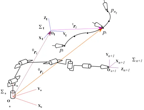
The task of a n-dof manipulator is specified by a set of ntm-dimensional vectors of operational
coor-dinates of the end-effector in an orthonormal fra-me åt. The manipulator considered is assumed as being redundant (n>m). The nt vectors correspond
to a sample of points pi (i = 1, 2, …, nt ) of the
desired path in the task space. The operational coor-dinates are the desired positions and orientations of the frame ån+1 attached to the end-effector, as showed in figure 1.
A suitable index of performance is then assigned by the user to one arbitrary path point, say pk , k Î {1,..., nt}, which must be maximized
by the corresponding manipulator’s configuration when the task will be accomplished. A law of motion is also given which refers to the time the position of the end effector on the path.
S
0Xo O
o Z o
Yo Xt
S
tYt O t Zt
p
1p
ip
n t
• •
•
•
• ••
•
S
n+1 Xn+1 Yn+1 Zn+1•
•
• • • ••
•
•
•
•
•
O n+1
t
r
i 0r
t 0r
iOn the other hand, the path placement is specified by variables regarding the position and orientation of the frame åt with respect to the frame å0 fixed to the base of the robot. They are the components of the placement vector defined as
[
]
0
e r rtx ty rtz
T
= , , , , ,a b g (9)
where rtx, rty, rtz, are the orthogonal components of
the vector of position ort (Figure 1), and a, b, g are the Euler angles Z-Y-X defining the orientation of åt with respect to the frame å0 .
It is desired to obtain the components of the placement vector 0e of the path, so that the index of manipulator’s kinematic performance associa-ted to the sample point pk is optimized when the
task is accomplished.
B. Process of solu tion
The single-objective problem is equivalent to a cons-trained non-linear programming problem. The ob-jective function is defined as the index of per-formance hk(qk) assigned to the path point pk. The
number of independent variables will be generally 6+n: the 6 components of the placement vector 0e of the path and, because of the manipulator’s redundancy, the n joint variables of the configu-ration qk which allow to satisfy the desired
situa-tion of the end-effector at the path point pk.
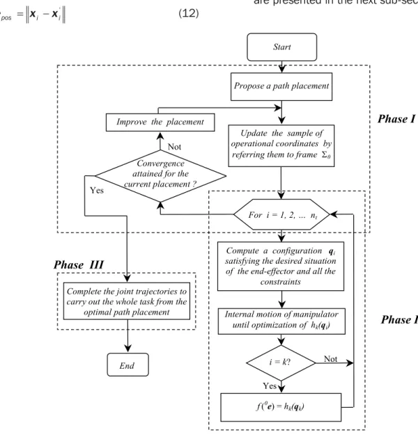
To solve the problem, we propose an optimi-zation process in three phases: phase I in which the optimal placement vector must be found; phase II addressed to compute the optimal confi-guration on the path point pk for each proposed
placement to be evaluated; and phase III commi-tted to complete the manipulator’s joint trajectories for the whole desired path by using the optimal path placement obtained in phase I. Notice that phase II allows to evaluate the objective function of phase I. Such a function in phase I can be defined as
f =hk(qk) (10)
The general procedure to solve the single-objective problem is schematized in the flow chart of figure 2. Details on the three phases concerned are given below.
Phase I
Before obtain the configurations at each path point, the operational coordinates must be referred to frame Ó0. Therefore, when a new placement is
proposed in the optimization process, the opera-tional coordinates have to be first updated in phase I by applying the following transformation:
0 i 0 t t i
T = T T (11)
In this equation: t
i
Tis the homo ge neous matrix estab lishing the desired posi tion and orien ta tion of the end effector on the path point pi referred to frame
t
å
.0T
t is the homo ge neous matrix for the posi tion and orien ta tion of frame
å
t referred to frameå
0. 0Ti is the homo ge neous matrix defining the posi -tion and orien ta -tion of the end effector on the path point pi with respect to frame
å
0.When the given operational coordinates have been updated, then the objective function must be evaluated in phase II for the current placement; after the process returns to phase I in order to check for the convergence of the method. If the convergence is attained then the procedure goes to phase III; otherwise, the placement must be improved by applying a suitable strategy.
Phase II
After updating of the operational coordinates for a path placement proposed in phase I, the redun- dancy must be solved to find the configurations qi
(i=1, 2, …. nt) for all the path points. To do that,
optimization of the same index of performance considered on pk; i.e., for one path point the
manipulator has to achieve the corresponding ope- rational coordinates and also optimize hk(qi). To
find such configurations the following process is carried out:
1. Find a configuration qi at each path point
in such a way that Equation (1) is satisfied. This configuration is obtained by minimization of the following function:
epos = xi -xi
' (12)
where xi is the vector defining the desired situation of the end-effector at point pi , and xi’is a vector of
operational coordinates corresponding to a confi-guration qi’ proposed when minimizing of equation (12). The symbol × denotes the Euclidean norm. If the task is feasible then equation x i = x i’ will be satisfied when the norm of equation (12) is mini-mized. The numeric minimization is carried out by applying a method of constrained non-linear opti-mization. The independent variables are the joint variables of qi’. The constraints to be considered are presented in the next sub-section.
236 INGENIERIA Investigación y Tecnología FI-UNAM
Phase II Phase I
Yes i = k?
Internal motion of manipulator until optimization of hk(qi)
f (0e) = hk(qk) Not Propose a path placement
Compute a configuration qi satisfying the desired situation of the end-effector and all the
constraints Update the sample of operational coordinates by referring them to frame S0
For i = 1, 2, … nt Improve the placement
Start
Not
Convergence attained for the current placement ?
End Yes
Complete the joint trajectories to carry out the whole task from the
optimal path placement
Phase III
2. When a configuration qi at one path point
has been found, satisfying both equation (1) and all the constraints, then compute J, J+and, Ñh( )q
and optimize for such a configuration the index h(q) by successively obtaining of the homogeneous solution of equation (3). At each iteration of this process, when a vector q&i of the homogeneous so-lution is obtained corresponding to a certain confi-guration qi, an improved configuration qi* may be
computed by
qi* =qi + Dq&i t (13) where D is a sufficiently small time interval. Note that, because q&i is a homogeneous solution, the improved configuration qi* will also preserve equa-tion (1). The initial configuraequa-tion of the optimizaequa-tion process has been determined in step i.
3. For one path-point the optimization of a confi-guration is stopped when Ñh( )q becomes zero.
Phase III
When computing the optimal path placement only a significant sample of path points is considered in order to reduce the time of computation engaged in the optimization process. Nevertheless, the de-sired trajectory is a continuous curve which must be approximated by a sufficiently large number of supplementary points of the path. So, to syn-thesize continuous joint trajectories for the whole task, when the optimal placement has been found the redundancy must be solved for supplementary path points. This process is the same used to solve the redundancy in phase II by optimizing the de-sired index of performance hk(q). The number of
sup-plementary points is proposed by the user in such a way that a conventional precision be satisfied. Con- tinuous joint trajectories will be obtained as a result of this process because the index to be optimized is the same for all the considered points.
C. Constraints of the problem
The optimization processes to obtain the path pla-cement and to solve the redundancy must be
constrained in order to obtain realistic solutions. The following constraints are taken into account:
1. Explicit constraints in phase I
Explicit constraints are imposed in phase I on the placement vector so that solutions are obtained only into the available physical space for the task placement. Such space may be imposed by a positioner device. The following constraints on the components of the placement vector are considered:
rt x l( ) rt x rt x u( )
0 £ 0 £ 0 (14a)
rt y l( ) rt y rt y u( )
0 £ 0 £ 0 (14b)
rt z l( ) rt z rt z u( )
0 £ 0 £ 0 (14c) a( )l £a £a( )u (14d)
b( )l £ £b b( )u (14e)
g( )l £ £g g( )u (14f)
In expressions (14), the indexes l and u denote, respectively, lower and upper bounds of the inde-pendent variables.
2. Implicit constraints in phase I for access to the task
Implicit constraints are also considered in order to guarantee the efficacy of placements proposed in the optimization process. To assure the accessi-bility to all the sample points on the path the following constraint is introduced:
ti £tu i=1 2, ,...,nt (15) where t i is the reach vector demanded to the manipulator at point pi; the symbol × denotes
Euclidean norm. tu is the norm of the maximum
3. Explicit constraints in phase II for joint limits avoidance
An elemental condition for any feasible configu-ration consists in preserving the joint variables into the admissible domain of configurations. So, any configuration used for the task should verify the following conditions:
qil q q i n j n
ij i
u
t
( ) £ £ ( ) =1,..., ; =1,..., (16)
where:
qij is the i-th joint vari able of the q j manipulator’s
config u ra tion corre sponding to the j-th task point. q qil
i u
( ) ( ) are the lower and upper limits, respecti-vely, of the i-th joint vari able.
4. Implicit constraints in phase II to guarantee continuous joint trajectories
Implicit constraints are imposed in phase II which allow to assure the feasibility of the whole joint tra-jectories.
To introduce the considered constraints we re-call here de notion of the aspect of a manipulator. One aspect is defined (Borrel et al., 1986) as a continuous subset of the manipulator’s joint space composed by configurations which render non-zero all the m-order minors of the jacobian matrix, except those minors being zero everywhere in the joint space.
Thus, the aspects of a manipulator are subsets of the joint space separated by hypersurfaces whose equations are determined by the m-order minors of the jacobian matrix equalized to zero.
On the other hand, it is known that for non-cus-pidal manipulators (Burdick et al., 1995), (Wenger, 1997), the continuity of joint trajectories corres-ponding to a given task can be guaranteed if the manipulator is constrained to use configurations remaining in only one aspect of its joint space.
Consequently, to guarantee continuous joint tra-jectories the following conditions must be imposed to manipulator’s configurations which will be used to accomplish a desired path:
e dkj kj( )q >0 (17)
where
dkj( )q is the left hand func tion of the equa tion defining the j-th hypersurface ( j = 1, 2,..., nhk )
whichborders the aspect Ak in the joint space;
kÎ {1, 2, ... , n A}. nhk is the number of such
hypersurfaces. nA is the number of the robot’s
aspects. Only one aspect will be chosen con-taining all the config u ra tions which allow to achieve the desired task.
ekj is a constant (+1 or –1) depending on the hypersurface and the consid ered as pect Ak.
In section VI we will identify the implicit cons-traints (17) for two manipulators.
VI. Optimal path placement for multi-objec tive optimization
A. State ment of the problem
The task of a n-dof manipulator is specified by a set of nt m-dimensional vectors of operational
coordi-nates of the end-effector (n>m) in an orthonormal frame
å
t. Such operational coordinates give thedesired positions and orientations to be followed by a frame
å
n+1 attached to the end-effector, as showed in figure 1. In that figure a sample of points pi (i = 1, 2, …, nt ) is illustratedcorres-ponding to the desired path in the task space. Suitable indexes of performance are then assig-ned by the user to several path points pi. Thus, we
want to compute the path placement vector 0e, so that all the indexes associated to the sample points be optimized while the task is being accom- plished. A law of motion is also specified which refers to the time and position of the end-effector on the path.
B. Process of solu tion
The multi-objective problem is also a constrained non-linear programming problem. The objective function should consistently characterize a set of dissimilar indexes of performance to be optimized. Thus, it is required that the indexes be first nor-malized to eliminate scaling and unity differences; then they can be included in a coherent objective function.
As in the single-objective problem, the inde-pendent variables will be the 6 components of the path placement vector 0e and, because of the manipulator’s redundancy, the joint variables of configurations qi which allow to satisfy the desired
situation of the end-effector on the path points pi.
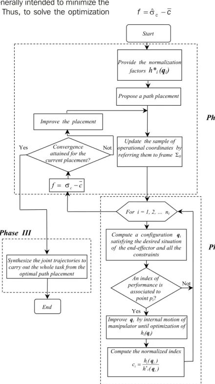
To solve the multi-objective problem we propose an optimization process having also three phases. In phase I the optimal placement will be searched; phase II is addressed to compute the optimal configurations at the nt path points for each
pla-cement to be evaluated; phase III is finally com-mitted to synthesize the manipulator’s joint trajectories for the whole desired path by using the optimal path placement obtained in phase I. Note that phase II allows to evaluate the objective function of phase I. Such a function is defined below. The procedure presented here to solve the multiobjective problem is illustrated in the flow chart of Figure 3. Details of the procedure are discussed in the next paragraphs.
Phase I
The path placement must be searched in this phase. For each placement proposed here we have to update the operational coordinates; then an evaluation of the placement can be accomplished in the process of optimization.
The transformation of such coordinates is carried out by applying equation (11); then the redundancy will be solved in phase II, and the objective function will be computed based on normalized indexes of performance. After that the
process returns to Phase I in order to check for the convergence of the method. If the convergence is attained then the procedure goes to Phase III; otherwise, the placement must be improved by applying a suitable strategy. The objective function for the multi-objective problem as well as the normalized indexes, are defined below.
A normalized index of performance associated to the sample point pi is obtained as:
c h
h
i
i i
i
= ( ) *
q
iÎ{ , ,..., }1 2 nt (18)
The normalization factor hi
* in equation (18) is the maximum value of the index of performance at the point pi that can be obtained by the
ma-nipulator when only such index is optimized, and the accessibility to all the path points is satisfied. In fact, the normalization factor hi* is the optimal value obtained for the index hi(qi) in the
sin-gle-objective problem. Thus, to obtain the normali-zation factors we have to solve as much single-objective problems as sample-configurations are to be optimized. It must be observed that a sample-point could hold or not an index of performance associated to be optimized; thus, the number of indexes to be optimized can be lower or equal than nt.
The main idea to define the objective function is that the value of such function, corresponding to a path location, must be equivalent to a typical value of the set of normalized indices to be optimized. Such typical value can be defined as:
c= -c s$c (19) where c and s$c are, respectively, the mean and the
standard deviation of the set of normalized indexes associated to the sample points. Hence, the value of c obtained by equation (19) corresponds to a typically small value of the set of normalized in-dexes of the sample.
maximized, then the global maximization of the set of nt indexes would be obtained by maximization of
c. Nevertheless, algorithms in usual software for optimization are generally intended to minimize the objective function. Thus, to solve the optimization
problem by minimization, the objective function could be defined as – c; therefore, such a function can be finally written as:
f =s$c -c (20)
240 INGENIERIA Investigación y Tecnología FI-UNAM
Phase II Phase I
Propose a path placement
Update the sample of operational coordinates by referring them to frame S0
Improve the placement
Start
Not Convergence
attained for the current placement? Yes
End
Synthesize the joint trajectories to carry out the whole task from the
optimal path placement
Phase III
Provide the normalization factors h*i (qi)
Improve qi by internal motion of
manipulator until optimization of hi(qi)
Compute a configuration qi
satisfyingthe desired situation of the end-effector andall the
constraints For i = 1, 2, … nt
Compute the normalized index
) ( h
) ( h c
i i
i i i
q q
*
= c
f = s)c
-Yes An index of performance is
associated to point pi?
Not
Phase II
The nt optimal configurations satisfying the desired
task and constraints, which are used to compute the normalized indexes, must be found in phase II. The algorithm to compute such configurations is the same used in single-objective problem; this one has been described in section III.
Phase III
The continuous joint trajectories for the whole task must be finally synthesized in Phase III for the op-timal path placement. To do that, the redundancy has to be solved for supplementary path points in such a way that the optimal configurations of points pi obtained in phase II are preserved.
In the multi-objective problem however, because of generally different indexes of performance are associated to adjacent sample path points, say pi
and pi+1, we cannot use a single index to solve the
redundancy by using the homogeneous solution for intermediate path points. In fact, if the homo-geneous solution is applied on intermediate points to optimize the index associated to pi, then the
joint trajectories becomes discontinuous on pi+1
and vice versa.
To solve the redundancy and synthesize the continuous joint trajectories connecting adjacent sample path points, a judicious strategy must be used. We propose a suitable secondary task to be accomplished, which is specified in the joint space as a continuous trajectory between configurations asso- ciated to adjacent sample path points. This secondary trajectory is such that the determinant of
J JT smoothly evolves from its value on point pi to
the value on point pi+1. Consequently, because all
the configurations so obtained belong to only one aspect, the continuity of joint trajectories will be assured. Thus, to accomplish both the main and the secondary tasks, we propose to solve the re-dundancy by minimizing the following objective function at each intermediate point pj between two
successive sample points pi and pi+1 :
f j epos j e j n
J
*
det * , , ,..., int
= + J =1 2 (21)
where nint is the number of intermediate points to
be considered between two sample points. This number is chosen by the user so that a con-ventional precision be satisfied. The error of posi-tion of the end-effector, epos j, in equation (21), is
defined like in equation (12) for intermediate points.
On the other hand, we define J*j =J Jj jT, where Jj
is the Jacobian matrix of the manipulator on the intermediate point pj. Then the error of the
determinant of J*
j in equation (21) is defined as
{
}
e abs j J J det * * ' * ( )J = detJ -det J (22) where:
det J*J is the desired value of the deter mi nant of J*
for the config u ra tion at point pj. Its value is
assigned by a cycloidal law [Equa tion (23)] which is defined for the current segment of the path between two succes sive sample points. Such cycloidal law must smoothly change the
deter mi nant of J* from its value corre sponding
to the config u ra tion at point pi, to that one at
pi+1 .
det( ' )J*
J is the value of the deter mi nant of J* for
the current config u ra tion in minimization of
equa tion 21.
The desired behavior of the determinant of J* in
the segment between sample points pi and pi+1 is
described by the following cycloidal law:
detJ*J =det Ji* +
(23) D
D D
(detJ' i* 'pj '
i pj i t T sen t T - æ è ç ç ö ø ÷ ÷ é ë ê ê ù û ú ú 1 2 2 p p
The variables concerned in equation (23) are defined as follows:
D(detJ*' detJ* det J*
t'pj =tpj -tpi DTi =tpi+1 -tpi
where tpi, tpj are the values of the time elapsed
when the end-effector arrives at points pi(sample)
and pj (intermediate), respectively.
C. Constraints of the problem
As considered for the single-objective problem, to obtain realistic solutions in solving the multi-ob-jective problem, explicit and implicit constraints should also be taken into account. Such cons-traints are identical to those considered in Section III C. They were examined in that section.
V. Path placement for global optimization The path placement problem was studied in sec-tion III for the optimizasec-tion of manipulator’s per-formance on a certain point of the path by taking into account a single kinematic criterion. Never-theless, in some tasks the optimization of such criterion can be preferred not only on a particular point but on every one of points in the path; i.e. a global optimization of manipulator’s performances is desired when the task is carried out. Note that such problem can be considered as a particular case of the multi-objective problem examined in the previous section. In fact, in the formulation for multi-objective optimization we can assign the sa-me criterion of performance to all the sample points in order to attain the global optimization. However, it must be pointed out that the homo-genization of the corresponding indices is not re-quired in the process of solution; then equation (18) takes the form ci =hi(qi).
Furthermore, after optimizing the set of indexes on the sample points, the continuous trajectories of joint variables for the whole path can be syn-thesized by applying only the Phase III of the pro-cess for the single-objective problem. Conse-quently, the minimization of function (21) is not ne-cessary for global optimization.
VI. Case studies
Several case studies are presented in this section in which single and multi-objective problems of optimal path placement are solved; we consider planar and spatial paths for each kind of problem. The planar task must be accomplished by a 3R ma- nipulator, and the spatial task should be achieved by a 4R manipulator. In the following sub-section, the geometric parameters of both manipulators will be specified and the implicit constraints of the problems to hold configurations in an aspect will be identified. Then, in succeeding subsections the pro-blems will be solved.
A. Manip u la tors for the case studies
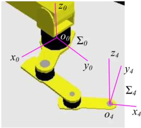
1. The 3R manipulator
The considered planar manipulator is shown in Figure 4, and its geometric parameters are pre-sented in table 1. These parameters are defined by using the modified Denavit-Hartenberg method (Khalil et al., 1986). A frame
å
4 is attached at the tip of the third link in order to use its origin to specify the linear velocity of the end-effector. The manipulator’s joint variables are è1, è2 and è3, andits limit values are q( )il = -150 and ° q i
u
( ) =150 , ° for i = 1, 2, 3 .
242 INGENIERIA Investigación y Tecnología FI-UNAM
x
4y
4z
4o
4Ó
4x
0z
0y
0Ó0
o
0By considering the velocity vector of O4 referred to the frame
å
0 as x& =[x y&,&]T, the jacobian matrix of the manipulator is:
J= - + + - +
-+ +
( ) | ( ) |
( )
s s s d s s d s d
c c c
1 12 123 12 123 123
1 12 123 d c|( 12 +c123) |d c123 d
é ë
ê ù
û ú
(24) In this matrix and hereafter we use the following compact notation:
cijk ºcos(qi +qj +qk) sijk ºsin(qi +qj +qk)
cij ºcos(qi +qj) sij ºsin(qi +qj) ci ºcos( )qi si ºsin( )qi
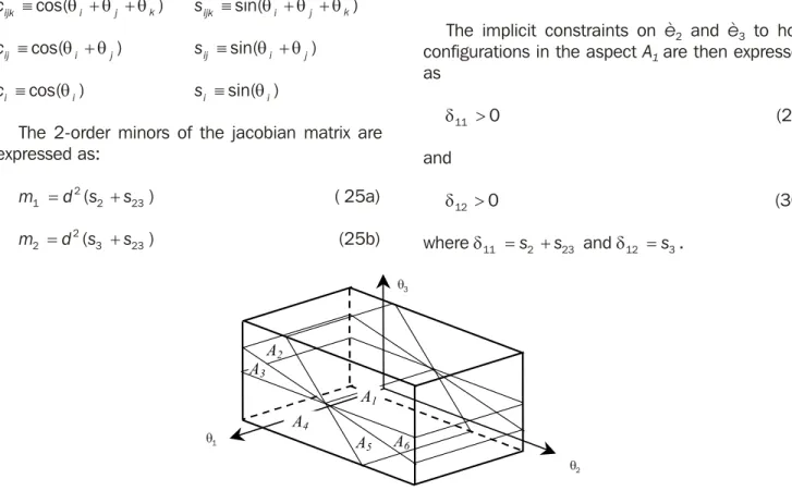
The 2-order minors of the jacobian matrix are expressed as:
m1 d s2 s 2 23
= ( + ) ( 25a)
m2 d s2 s 3 23
= ( + ) (25b)
m3 d s2 3
= (25c)
The conditions of configurations which render zero the above minors provide the following equa-tions of the surfaces dividing the joint space in aspects:
s2 +s23 =0 (26) s3 +s23 =0 (27) s3 =0 (28) Thus, six aspects can be identified (nA=6) for
the 3R manipulator, as showed in figure 5. We chose the aspect A1 for the achievement of the
task; consequently for (17) we have k=1. Then we observe that the aspect A1 is surrounded by the
surfaces specified by equations (26) and (28); therefore we have nhk =2 and å11=1, å12=1 for
ine- quality (17).
The implicit constraints on è2 and è3 to hold
configurations in the aspect A1 are then expressed
as
d11 >0 (29)
and
d12 >0 (30)
where d11 =s2 +s23 and d12 =s3.
Table 1. Geometric param e ters of the 3R manip u lator
a d q r
1 0 0 q1 0
2 0 d q2 r2
3 0 d q3 r3
4 0 d 0 0
A6
1) q
2
A2
A5
A3
A1
A4
q3
q1
q2
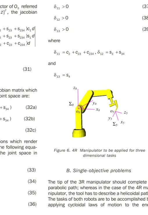
2. The 4R manip u lator
The manipulator is shown in figure 6 and its geo-metric parameters are presented in table 2. The joint variables are è1, è2, è3 and è4, and its limits
values are q( )il = -150 and ° q i
u
( ) =150 , for i = 1,° 2, 3, 4. To specify the linear velocity of the end effector we use the point O5 of the frame
å
5 which is attached at the tip of the fourth link.By considering the velocity vector of O5 referred to the frame
å
0 as x& =[x y z& &, ,&]T, the jacobian matrix of the 4R manipulator is:
J= - + + + + é ë ê ê ê - + + ( ) ( ) (
c c c s d
c c c c d
s s 2 23 234 1
2 23 234 1
2 23
0
s c d
s s s s d
c c c d
234 1
2 23 234 1
2 23 234 ) ( ) ( ) - + + + + - + - + + -( ) ) ( )
s s c d
s s s d
c c d
s c d s 23 234 1
23 234 1
23 234 234 1 234 1 234 s d c d ù û ú ú ú (31)
The 3-order minors of the jacobian matrix which are non zero everywhere in the joint space are: m1 d3 c c c s s 2 23 234 3 34 = - ( + + )( + ) (32a) m2 d3 c c c s s 2 23 234 4 34 = - ( + + )( + ) (32b) m3 d s c3 c c 4 2 23 234 = - ( + + ) (32c) The conditions of configurations which render zero the above minors provide the following equa-tions of the surfaces dividing the joint space in aspects: c2 +c23 +c234 =0 (33)
s3 +s34 =0 (34)
s4 +s34 =0 (35)
s4 =0 (36)
Thus, twelve aspects can be identified (nA=12) for the 4R manipulator. We chose the aspect A1 for the achievement of the task; consequently, for inequality (17) we have k=1. Then we observe that the aspect A1 is bounded by the surfaces of equations (33), (34) and (36); therefore for inequality (17) we have nhk =3 and å11=1, å12=1, å13=1. Thus, the implicit constraints on configu-rations to hold configuconfigu-rations in the aspect A1 are: d11 >0 (37)
d12 >0 (38)
d13 >0 (39)
where
d11 =c2 +c23 +c234,d12 =s3 +s34
and d13 =s4
B. Single-objective prob lems
The tip of the 3R manipulator should complete a parabolic path; whereas in the case of the 4R ma-nipulator, the tool has to describe a helicoidal path. The tasks of both robots are to be accomplished by applying cycloidal laws of motion to the
end-244 INGENIERIA Investigación y Tecnología FI-UNAM x0 z0 y0 Ó0 o0 x5 y5 Ó5 z5 o5
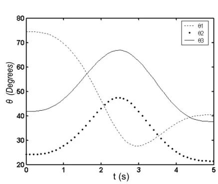
effector during 5 seconds. The Cartesian coordi-nates of the sample-points are referred to the frame åt; they are given in tables 3 and 5. In the two cases the path placements must be deter-mined in such a way that the manipulability index is maximized on the point p3 (when t=2.5 s). The
independent variables of the planar problem are rtox, rtoy , and a (rotation about the axis z0 ); in the
case of the 3D path, the additional variable rtoz
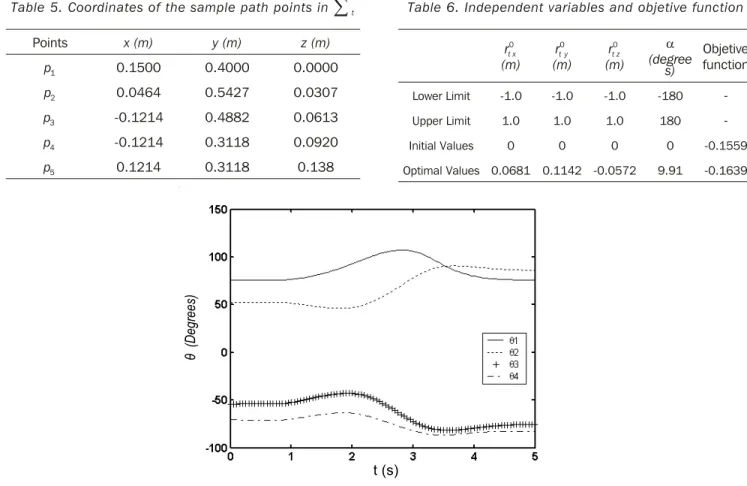
must be included. The initial values for such va-riables, as well as the obtained optimal values are given in tables 4 and 6. In the same tables the initial and a the optimal values of the objective functions are presented. The joint trajectories corresponding to the optimal placement are observed in figures 7 and 10. The behaviors of the normalized manipulability are compared in figures 8 and 11. Sequences of configurations of the robots during the accomplishment of the tasks are presented in figures 9 and 12 for the initial and the optimal placements.
Table 3. Coor di nates of the sample path points in
å
tPoints x (m) y (m)
p1 -0.2785 0.5028
p2 -0.1392 0.3856
p3 0.0000 0.3504
p4 0.1392 0.3970
p5 0.2547 0.4979
Table 4. Inde pendent vari ables and objetive func tion
rt x
0
(m)
rt y
0
(m)
a
(degrees)
Objetive function
Lower Limit -1.0 -1.0 -90
-Upper Limit 1.0 1.0 90
-Initial Values 0 0 0 -0.1233
Optimal Values 0.0492 0.2405 -1.93 -0.1723
t (s)
è
(D
eg
re
es
)
B1. Para bolic path
246 INGENIERIA Investigación y Tecnología FI-UNAM
t (s)
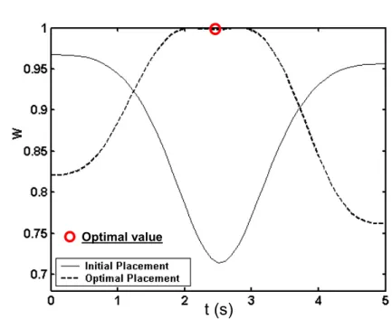
Optimal value
Figure 8. Normal ized manipulability of the 3R manip u lator for the planar task
t=0 s t=2 s t=2.5 s t=5 s
a) Initial placement:
t=0 s t=2 s t=2.5 s t=5 s
b) Optimal placement:
è
(D
eg
re
es
)
t (s)
Figure 10. History of joint vari ables for the optimal place ment. 4R manip u lator. Single crite rion.
t (s)
Optimal value
Figure 11. Normal ized manipulability of the 4R manip u lator during the task Table 5. Coor di nates of the sample path points in
å
tPoints x (m) y (m) z (m)
p1 0.1500 0.4000 0.0000
p2 0.0464 0.5427 0.0307
p3 -0.1214 0.4882 0.0613
p4 -0.1214 0.3118 0.0920
p5 0.1214 0.3118 0.138
Table 6. Inde pendent vari ables and objetive func tion
rt x
0
(m) rt y
0
(m) rt z
0
(m)
a
(degree s)
Objetive function
Lower Limit -1.0 -1.0 -1.0 -180
-Upper Limit 1.0 1.0 1.0 180
-Initial Values 0 0 0 0 -0.1559
C. Multi-objective prob lems
In the case of the planar task the extremity of the 3R manipulator should complete a parabolic path; for the 3D task the 4R manipulator’s tool has to describe a helicoidal path. In both cases the mo-tion of the end-effector follows a cycloidal law. The periods of the tasks are 6 and 5 seconds for the 3R and 4R manipulators, respectively. The Cartesian coordinates of the sample-points are referred to frame åt, and different indexes of performance are associated to some points, as indicated in tables 7 and 10. In the problems we want to determine the path placement which allows to optimize the value of the specified indexes by the related manipu-lator’s configuration when the task is carried out.
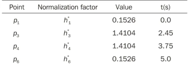
The normalization factors used in equation (18) are previously computed by solving the single-objective problem for points having a related index of performance. The obtained values of such fac-tors are listed in tables 8 and 11. The independent
variables of the planar problem are rtox , rtoy , and a
(rotation about the axis z0 ); in the case of the 3D path, the additional variable rtoy must be included.
The initial values for such variables, as well as the obtained optimal values are given in tables 9 and 12. In the same tables the initial and optimal va-lues of the objective functions are presented. The joint trajectories corresponding to the optimal placement are observed in figures 13 and 18. The progress attained of the normalized indices asso-ciated to the sample points can be appreasso-ciated in figures 14 and 19. The behaviors of the manipu-lability and the condition number (both normalized) during the task are shown in figures 15, 16, 20 and 21. Sequences of configurations of the robots describing the desired paths are presented in figures 17 and 22 for the initial and the optimal placements.
248 INGENIERIA Investigación y Tecnología FI-UNAM a) Initial placement:
b) Optimal placement:
t=5 s t=3 s
t=0 s t=2.5 s
t=5 s t=3 s
t=0 s t=2.5 s
Table 8. Normal iza tion factors and time asso ci ated to the sample points
Point Normalization
factor Value t (s)
p1 h1*
0.1727 0.0
p3 h3
*
1.0841 3.5
p5 h5
* 1.0841 5.0
p6 h6
* 0.1727 6.0
Table 10. Coor di nates of the sample path points in
å
tPoint x (m) y (m) z (m) Index of
performance
p1 0.3722 0.1466 0.1126 Manipulability
p2 0.3587 0.1770 0.1375
-p3 0.0935 0.3889 0.4005 Condition number
p4 -0.2330 0.3251 0.6578 Condition
number
p5 -0.2554 0.3079 0.6790
-p6 -0.2876 0.2780 0.7120 Manipulability
Table 11. Normal iza tion factors and time asso ci ated to the sample points
Point Normalization factor Value t(s)
p1 h*1
0.1526 0.0
p3 h3
*
1.4104 2.45
p4 h4
* 1.4104 3.75
p6 h6
* 0.1526 5.0
Table 12. Inde pendent vari ables and objective
rt x o
(m) rt y
o
(m) rt z
o
(m) a (degrees) Objective function
Lower Limit -1.0000 -1.0000 -1.0000 -180.0
-Upper Limit 1.0000 1.0000 1.0000 180.0
-Initial Values 0.0000 0.0000 0.0000 0.0 -0.3537
Optimal Values 0.0865 0.1233 -0.2438 16.8 -0.6635
Table 9. Inde pendent vari ables and objec tive function
rt x
0 r
t y
0 a (degrees)
Objective function
Lower Limit -1.0000 -1.0000 -90.0
-Upper Limit 1.0000 1.0000 90.0
-Initial Values 0.4000 0.1000 30.0 -0.5967
Optimal Values -0.0206 -0.0378 -11.0 -0.8922
Table 7. Coor di nates of the sample path points in
å
tPoint x (m) y (m) Index of
performance
p1 -0.2785 0.5029 Manipulability
p2 -0.2390 0.4614
-p3 0.0872 0.3701 Condition number
p4 0.1614 0.4143
-p5 0.2424 0.4845 Condition number
p6 0.2548 0.4979 Manipulability 1. Para bolic path
250 INGENIERIA Investigación y Tecnología FI-UNAM
p
1c
p
6p
5p
3Point
Figure 14. Values of the normal ized indices
è
(D
eg
re
es
)
t (s)
t (s)
Optimal values
Figure 16. Behavior of the normal ized condi tion number during the task
t (s)
Optimal values
Figure 15. Behavior of the normal ized manipulability during the task
252 INGENIERIA Investigación y Tecnología FI-UNAM
è
(
D
eg
re
es
)
t (s)
Figure 18. History of joint vari ables for the optimal place ment. 4R manip u lator. Multi-criteria Figure 17. Simulation of the task
b) Optimal placement: a) Initial placement:
t=0 s t=3.5 s t=5 s t=6 s
t=0 s t=3.5 s t=5 s t=6 s
Optimal values
t (s)
Figure 20. Behavior of the normal ized manipulability during the task
p
1p
6Point
p
3p
4254 INGENIERIA Investigación y Tecnología FI-UNAM
t=5 s t=0 s
t=3.75 s t=2.45 s
b) Optimal placement: a) Initial placement:
t=5 s
t=0 s t=2.45 s t=3.75 s
Figure 22. Simu la tion of the task
t (s)
Optimal values
Conclu sion
General formulations were presented in this paper to determine the best position and orientation of a path to be followed by a redundant robotic mani-pulator. Depending on the requirements of the user, the quality of a placement can be measured by using either a single criterion or multiple criteria of manipulator’s performance. Consequently, the proposed formulations are addressed to solve both single and multi-objective optimization problems. In the single-objective problem, one index of per-formance associated to a specific path-point is defined as the function to be optimized. On the other hand, in the multi-objective problem such a function is equivalent to a characteristic index which represents the set of normalized indexes to be optimized. The proposed formulations take into account constraints regarding the accessibility to the manipulator’s task. Indeed, we introduce cons- traints in order to: a) demarcate an available phy-sical space to locate the task; b) avoid trans-gression of joint limits during the accomplishment of the task; c) generate continuous joint trajec-tories on the whole task.
The case studies examined here showed that significant improvements of the manipulator’s per-formance can be obtained by applying our approach. In such cases all the constraints were satisfied and consequently the accessibility to the complete tasks was assured. However, in the hypothetical case in which a satisfactory solution could not be found by trying with a first mani- pulator’s aspect, then further attempts could be accomplished by using other manipulator’s aspects to satisfy the accessibility conditions and improve the mani-pulator’s performance. On the other hand, the sample points considered in the problems were chosen by using a criterion of symmetry; never-theless, both the number of points and the position of such points on the path could have an influence on the level of the improvement obtained for the indices of performance. Thus, supplementary stu-dies should be carried out to characterize a sui-table criterion to solve both questions. Furthermore,
in future works additional constraints will be taken into account to avoid collisions of the manipulator when it works in cluttered environments.
Acknowl edg ments
The sub ven tion for co op er a tion be tween re search -ers of the Instituto Tecnológico de la Laguna of Mex ico and the Laboratoire de Mécanique des Solides of France for this work was made pos si ble under the grant M00 M02 ECOS-CONACyT-ANUIES. On the other hand, a part of the pres ent work was sup ported by the Na tional Coun cil of Sci ence and Technology –CONACyT– of Mex ico, (grant 31948-A).
Refer ences
Abdel-Malek S. and Nenchev D.N. Local torque minimization for redun dant manip u la tors: a correct formu la tion. Robotica, 14:235-239, 2000.
Angeles J. and López-Cajún C. Kine matic isotropy and condi tioning index of serial robotic manip u -la tors. Int. J. Robotics Research, 11(6):560-571, 1992.
Aspragathos N.A. and Foussias S.Optimal loca tion of a robot path when consid ering velocity perfor -mance. Robotica, 20:139-147, 2002.
Borrel B. and Liegois A. A study of multiple manip u -lator inverse kine matic solu tion with appli ca -tions to trajec tory plan ning and workspace de-termi na tion. IEEE Proc. of the 1986 International Confer ence on Robotics and Auto ma -tion, pp. 1180-1185.
Burdick J.W. A clas si fi ca tion of 3R regional manip u
-lator singu lar i ties and geom e tries. Mech a nisms
and Machine Theory, 30(1):71-89, 1995.
Chiu S.L. Task compat i bility of manip u la tors postu-res. Int J. Robotics Research, 7(5):13-21, 1988. El Omri J. and Wenger P. How to recog nize simply a
nonsingular posture changing 3DOF manip u -lator. Proceed ings of the 7th Inter na tional Con-ference on Advanced Robotics, 1995, pp. 215-222.
IEEE Proc. of the 21st Confer ence on Deci sion and Control, 1988, pp. 2280-2283.
Hemerle J.S. and Prinz F.B. Optimal path place -ment for kine mat i cally redun dant manip u la tors. Proceed ings of the 1991 IEEE Inter na tional Confer ence on Robotics and Auto ma tion, 1991, pp. 1234-1243.
Hsu D., Latombe J.C. and Sorkin S. Placing a robot manip u lator amid obsta cles for opti mized Exe-cution. IEEE Int. Symp. on Assembly and Task Planning, 1999.
Khalil W. and Kleinfinger J.F. A new geometric
nota tion for open and closed-loop robots. In:
Proceed ings of the IEEE Inter na tional
Confe-rence on Robotics and Auto ma tion, 1986, pp. 1174-1180.
Klein C.A. and Blaho, B.E. Dexterity measures for the design and control of kine mat i cally redun -dant manip u la tors. Int. J. Robotics Research, 6 (2):72-83, 1987.
Nakamura Y. and Hanafusa H. Optimal redun dancy control of robot manip u la tors. Int. J. Robotics Research, 6(1):32-42, 1987.
Ma S. and Nenchev D.N. Local torque minimi-zation for redun dant manip u la tors: a correct formu la tion. Robotica, (14):235-239, 1996. Nelson B., Pedersen K. and Donath M. Locating
assembly tasks in a manip u la tor’s workspace. IEEE Proc. of the Inter na tional Confer ence on Ro-botics and Auto ma tion, 1987, pp. 1367-1372. Pamanes G. J. A. A crite rion for optimal place ment of robotic manip u la tors. IFAC Proc. of the 6th Symp. on Infor ma tion Control Prob lems in Manu fac turing Tech nology, 1989, pp.183-187.
Pamanes G.J.A and Zeghloul S. Optimal place ment of robotic manip u la tors using multiple kine matic criteria. Proceed ings of the 1991 IEEE Inter na -tional Confer ence on Robotics and Auto ma tion, 1991, pp. 933-938.
Pamanes G.J.A., Barrón L.A. and Pinedo C. Cons-trained opti mi za tion in redun dancy reso lu tion of robotic manip u la tors. Proceed ings of the 10th World Congress on Theory of Machines and Me- chanisms, Oulu, Finland, 1999, pp. 1057-1066. Reynier F., Chedmail P. and Wenger P. Optimal posi tioning of robots: feasi bility of contin uous trajec to ries among obsta cles. IEEE Int. Conf .on Systems Man. and Cyber netics Proc., 1992. Wenger P. Design of cuspidal and noncuspidal ma-
nipulators. Proceed ings of the IEEE Inter na tional Confer ence on Robotics and Auto ma tion, 1997, pp 2172-2177.
Yoshikawa T. Manipulability of robotics mecha-nisms. Int. J. Robotics Research, 4(2):3-9, 1985. Yoshikawa T. and Kiriyama S. Fourjoint redun
-dant wrist mech a nism and its control. Jour-nal of Dynamic System, Measure ment, and Con-trol, 111:200-204, 1989.
Zeghloul S. and Pamanes G.J.A. Multi-criteria pla-cement of robots in constrained envi ron ments. Robotica, 11:105-110, 1993.
Zhou Z.L., Charles C. and Nguyen. Globally optimal trajec tory plan ning for redun dant manip u la -tors using state space augmen ta tion method. Journal of Intel li gent and Robotic Systems, Vol. 19(1):105-117, 1997.
Semblanza de los autores
J. Alfonso Pamanes-García. Was born in Torreon, Mexico, in 1953. He received the B.S. degree from the La Laguna Insti tute of Tech nology in 1978, the M.S. degree in mechanics in 1984 from the National Poly technic Insti tute of Mexico, and the Ph.D. degree in mechanics from the Poitiers Univer sity, France, in 1992. He is a professor in mechanics of robots at the La Laguna Insti tute of Tech nology, Torreon, Mexico. His research inter ests are in modeling and motion plan ning of robots. Author of more than 50 scien tific papers published in national or inter na tional congress and jour nals. He has been reviewer of the National Council of Science and Tech nology of Mexico for eval u a tion of national research projects.
Saïd Zeghloul. Received the M.S. degree in mechanics and the Ph.D. degree in robotics from the Univer sity of Poitiers, France, in 1980 and 1983, respec tively, and the Doctorat d’Etat es sciences physiques degree in 1991. He is a pro-fessor at the Faculte des Sciences of the Poitiers Univer sity where he teaches robotics. He is leader of the research group in robotics of the Laboratoire de Mecanique des Solides of Poitiers, where his research inter ests include mobile robot and manip u lator path planing, mechan ical hand grasp planing.