www.nonlin-processes-geophys.net/18/161/2011/ doi:10.5194/npg-18-161-2011
© Author(s) 2011. CC Attribution 3.0 License.
in Geophysics
Multi-scale interactions of geological processes during
mineralization: cascade dynamics model and multifractal
simulation
L. Yao1and Q. Cheng1,2
1State Key Laboratory of Geological Processes and Mineral Resources, China University of Geosciences,
Wuhan 430074, China
2Department of Earth and Space Science and Engineering, York University, Toronto, ON M3J1P3, Canada
Received: 3 January 2010 – Revised: 10 October 2010 – Accepted: 9 February 2011 – Published: 8 March 2011
Abstract. Relations between mineralization and certain geological processes are established mostly by geologist’s knowledge of field observations. However, these relations are descriptive and a quantitative model of how certain ge-ological processes strengthen or hinder mineralization is not clear, that is to say, the mechanism of the interactions be-tween mineralization and the geological framework has not been thoroughly studied. The dynamics behind these inter-actions are key in the understanding of fractal or multifractal formations caused by mineralization, among which singular-ities arise due to anomalous concentration of metals in nar-row space. From a statistical point of view, we think that cascade dynamics play an important role in mineralization and studying them can reveal the nature of the various inter-actions throughout the process. We have constructed a mul-tiplicative cascade model to simulate these dynamics. The probabilities of mineral deposit occurrences are used to rep-resent direct results of mineralization. Multifractal simula-tion of probabilities of mineral potential based on our model is exemplified by a case study dealing with hydrothermal gold deposits in southern Nova Scotia, Canada. The extent of the impacts of certain geological processes on gold mi-neralization is related to the scale of the cascade process, especially to the maximum cascade division numbernmax.
Our research helps to understand how the singularity occurs during mineralization, which remains unanswered up to now, and the simulation may provide a more accurate distribution of mineral deposit occurrences that can be used to improve the results of the weights of evidence model in mapping min-eral potential.
Correspondence to:Q. Cheng ([email protected])
1 Introduction
Mineralization has complex connections with various geo-logical processes and geologists can deduce part of these connections from outcrop exploration. For example, if cer-tain deposits are always coexisting with a special type of intrusion, we may consider that this intrusion is related to mineralization during geological periods. The summariza-tion of such relasummariza-tions between mineralizasummariza-tion and certain ge-ological processes and their gege-ological characteristics leads to metallogenic models for distinct genetic types of mineral deposits (Cox and Singer, 1986). Metallogenic models give a comprehensive knowledge of favourable conditions for mi-neralization, but they are far too insufficient to capture the mechanism of the interactions between mineralization and the geological framework, because they are inherently de-scriptive. Such a mechanism is indispensable as we wonder why common fractal or multifractal features has been formed throughout mineralization.
based on observations. Mineralization has been thought of as a self-organization process with dissipative structures and, thus, nonlinear features and complexities emerged (Yu et al., 1988), but the dynamical model of the process is too sen-sitive for the parameters that it is hard to characterise. A novel understanding of the mineralization is its interpretation as a singular event (Cheng, 2007b,a), which always results in multifractal products. Besides mineralization, typical singu-lar events include hazard events, such as earthquakes, land-slides, volcanoes, floods and hurricanes, because they result in anomalous amounts of energy release or mass accumula-tion confined to narrow intervals in space or time (Cheng, 2007b,a). However, the mechanism of mineralization as a singular event remains a puzzle.
Generally speaking, the dynamics of the interactions be-tween mineralization and the geological framework is still lacking in systematic research. The answer to the above question would aid in understanding why singularity occurs and the multi-scale nature of mineralization. In this paper, we construct a cascade model to simulate interactions between mineralization and the relevant geological processes. Then, a case study of hydrothermal gold mineral deposits in south-ern Nova Scotia, Canada is described for multifractal simu-lation, in which we use some statistics from Cheng (2008). Through our research, we think that mineralization may be accompanied by diverse geological processes, which exerted their impacts in a cascade-like manner and their impacts are associated with mineralization in different scales.
2 Multifractal and singularity
Since the fractal concept was proposed (Mandelbrot, 1977, 1983), fractal or multifractal methods became powerful tools for identifying geological features associated with minerali-zation. Fractal or multifractal modelling play important roles in the quantifying of mineral deposits (Turcotte, 1996), char-acterising the spatial distribution of mineral deposits (Carl-son, 1991; Agterberg et al., 1996; Raines, 2008) and map-ping mineral-potential (Cheng et al., 1996; Ford and Blenk-insop, 2008). New methods based on the multifractal the-ory, such as concentration-area (C-A) method (Cheng et al., 1994), spectrum-area (S-A) method (Cheng et al., 2000) and the singularity mapping technique (Cheng, 2007a), were de-veloped to identify geochemical anomalies and to map min-eral potential (Cheng, 2007b; Cheng and Agterberg, 2009; Zuo et al., 2009a).
While many mathematical geologists are familiar with multifractal spectrumf (α)in the model of Evertsz and Man-delbrot (1992); Schertzer and Lovejoy (1991), they devel-oped another multifractal model in geophysics based on codi-mension functionC(γ ), whereαandγ represent H¨older ex-ponent and field order, respectively. Cheng (1996) compared these two models. Here, we introduce the elementary nota-tions and formulas based on thef (α)model.
Suppose a geometrical support with linear sizeǫwas de-fined asA(ǫ), andµ[A(ǫ)]represents a kind of measure on A(ǫ), i.e., the most common measures of this kind related to mineralization may be the average geochemical concentra-tions on areas at different scales, then the following power-law relationships exist in conditions of multifractal:
µ[A(ǫ)]∝ǫα (1)
Nα(ǫ)∝ǫ−f (α) (ǫ→0) (2)
where ∝ means “proportional to”, α is singularity index, Nα(ǫ)is the number of cells having singularity indexαwhile ǫ approaches zero and f (α) is the multifractal spectrum. Equation (1) is scale-invariant because the singularity index αremains constant under all rescalings of the linear sizeǫ. If the size is changed fromǫn−1toǫnfor some scaleλ, that is,ǫn=λǫn−1, and the measure is changed fromµA(ǫn−1)
toµ[A(ǫn)], respectively, then the following can be obtained from Eq. (1):
µ[A(ǫn)]/µA(ǫn−1)=λα (3)
Actually fractal or multifractal describes the scale-invariant relationship of a kind of measure on another kind of measure. Thus, the above formulae can be extended to Lebesgue measure space, and the support can even be fractal itself (Falconer, 2003). In this study, posterior probabilities of mineral deposit occurrences on certain geological condi-tions and the probabilities of occurrences of the relevant geo-logical occurrences are Lebesgue measures, so their relation-ships can be multifractal only if the nonlinear interactions exist between them.
IfA(ǫ) is the volume in D-dimensional space, a fractal density (Cheng, 2008) can be deduced from Eq. (1) as:
ρ[A(ǫ)]∝µ[A(ǫ)]/A(ǫ)∝ǫα−D (4)
where fractal densityρis analogous to density in the physical sense, but this density changes with scale and can approach infinity; the index(α−D)also corresponds to the concept of codimension meaning the differences between the dimen-sions of space and fractal (Schertzer and Lovejoy, 1987).
3 Multiplicative cascade models and their multifractal effect
ξ
(1 +d)ξ (1−d)ξ
(1 +d)2ξ (1
−d)(1 +d)ξ (1−d)(1 +d)ξ (1−d)2ξ
. . .
· · ·
· · · ·
(1 +d)n
ξ · · · (1−d)
n
ξ
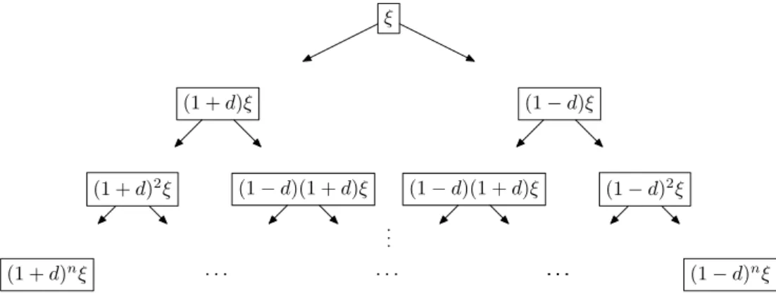
Fig. 1. 1-D multiplicative cascade model of De Wijs (De Wijs, 1951). Theξmeans original concentration value, anddis the dispersion coefficient.
later it was adopted as a binomial cascade model to simu-late multifractal (Mandelbrot, 1989). Various cascade mod-els have been used to simulate rainfalls, clouds and geochem-ical concentrations (Deidda, 1999; Lovejoy and Schertzer, 2006; Agterberg, 2001).
A cascade process redistributes the mass concentrated on an support to small pieces through a series of repeated steps, leading to scale-invariant results. Taking the De Wijs model of geochemical distribution as an example, if the original concentration isξ and the support is 1, then in the next it-eration, the support is divided into two equal blocks of 1/2 with a concentration of(1+d)ξ and(1−d)ξ; hered is the dispersion coefficient and is independent of block size; the procedure is iterated on the divided blocks (Fig. 1).
Generally considering a measure defined on a support, a basic cascade step includes two intertwining procedures: a partition procedure dividing current support into smaller parts while the scale drops down by a constant ratio; and a distribution procedure assigning different weights to the di-vided parts based on a probability distribution. The size of the ultimately divided supports would approach zero, while the cascade step is repeating endlessly. However, sometimes the cascade steps throughout a cascade process are limited and, thus, the ultimate size of the divided parts from the orig-inal support is determined by the divided times, which we denote as the maximum cascade division numbernmaxhere.
The measures allocated on the divided parts in each subdi-vision depend on the weights pattern for redistributing val-ues from previous results. The maximum cascade division numbernmaxis meaningful to geological processes because
it actually corresponds to the scale of a certain geological process. For example, the continental or ocean plate move-ment brings about global-scale change of geological settings, yet migrations of geochemical elements in a metallogenic province can only be on a regional-scale. To represent re-ality, many kinds of modifications on the basic model have been investigated. For example, Agterberg (2001) introduced minor disturbances in the cascade processes to simulate
geo-chemical map patterns and proposed a random-cut variant of the De Wijs model (Agterberg, 2007a), Cheng (2005) applied a cascade model with variable partition processes, Schertzer and Lovejoy (1987) developed a cascade model continuous in scale.
The results of cascade dynamics are multifractal. The multifractal generated by this cascade process have many lo-cal maxima and minima with different singularities (Cheng, 2008). As a 1-D multiplicative cascade process, the mini-mal singularityαminand maximal singularityαmaxand their
difference1αcan be calculated as: αmin=1−log2(1+d)
αmax=1+log2(1+d)
1α=αmax−αmin=log2
1+d
1−d (5)
wheredis the dispersion coefficient.
4 Quantification of nonlinear dynamical interactions throughout mineralization
4.1 Statistical model of mineralization by weights of evidence
geological processes comes from statistical analysis of vari-ous exploration data. The exploration data include observa-tions from mineral deposits, geological structures, geochem-ical concentrations, petrologgeochem-ical or stratigraphic formations and so on. A specific kind of exploration data actually repre-sents products of a certain geological process, and the min-eral deposits can be seen as results of minmin-eralization. There-fore, analysing the relationships between mineralization and other kinds of exploration data provides an approximation to quantify the dynamical interactions between them. There are already models to utilize and integrate these relationships in order to evaluate mineral potential, as we have mentioned in the previous section. We choose the weights of evidence (WofE) method, which is very popular for mapping mineral potential, to statistically quantify the relationships between mineralization and certain geological processes, because it is reasonable and easy to understand.
The WofE model treats each kind of exploration data as a separate evidential layer and then integrates the evidential layers to support the final decision. Each kind of exploration data corresponds to the result of a certain geological event. In particular, the mineral deposit occurrences are products of mineralization. The geological events having a positive correlation with occurrences of mineral deposits are called favourable events in mapping mineral potential. Evidential layers are usually raster grids made of discrete cells to facili-tate processing by GIS software in practice (Bonham-Carter, 1994). Each grid cell in an evidential layer falls into two distinct groups according to positive or negative correlation with occurrences of mineral deposits. Grid cells having pos-itive correlation with occurrences of mineral deposits consti-tute favourable areas, and the remaining grid cells consticonsti-tute unfavourable areas. Then the relationships between mine-ralization and certain geological events can be discussed by the posterior probabilities of mineral deposit occurrences on condition that these events occurred.
For simplicity, we use some specific symbols to represent formations of different geological events. We suppose the mineralization event asD and, as a result, the prior prob-ability of mineral deposit occurrence is known asP (D); a favourable event to mineralization is denoted asAand then the corresponding evidential layer is a binary pattern with Aor A˜ representing favourable events or not and, respec-tively, their probabilities of occurrences can be written as P (A)andP (A). Thus,˜ D would be divided into DA and DA, and the posterior probabilities can be represented by˜ P (D|AandP (D| ˜A), respectively. From Bayesian rule, the posterior probabilities can be calculated as
P (D|A)=P (D)P (A|D)
P (A)
PD| ˜A=P (D)P (A˜|D)
P (A)˜ . (6)
If evidential patterns representing favourable geological
events to mineralization are arranged asA1,A2,...,An, while the contrary complements are denoted asA˜1,A˜2,...,A˜n, then a more comprehensive relation can be derived as
P D|A1A2...An=
P (D)P (A1|D)P (A2|D)...P (An|D) P (A1)P (A2)...P (An)
PD| ˜A1A˜2...A˜n
=
P (D)PA˜1|D
PA˜2|D
...PA˜n|D
PA˜1
PA˜2
...PA˜n
.
(7) Note the Eqs. (7) require conditional independence assump-tion, which can be written as
P A1A2...An|D=P A1|DP A2|D...P An|D
PA˜1A˜2...A˜n|D
=PA˜1|D
PA˜2|D
...PA˜n|D
.(8)
The weights W+ and W− are then defined as follows (Agterberg et al., 1990):
W0=loge n
P (D)/P (D)˜ o
WA+=loge n
P (A|D)/P (A| ˜D)o
WA−=loge n
PA˜|D/PA˜| ˜Do. (9) Under the transformation of posterior probabilities by logit function, the logits of posterior probabilities of mineral de-posit occurrences associated with multiple layers of evidence can be derived from Eqs. (9) assuming that conditional inde-pendence is satisfied:
L(D|A1A2...An)=W0+WA1++WA2++...+WAn+ (10)
where L represents logit function and L(D|A1A2...An) means logit ofP (D|A1A2...An). The similar formulae can be derived under other combinations of evidential layers. The logit function is important to logistic regression and the logit of a numberpbetween 0 and 1 is given by the formula:
L(p)=log
p
1−p
. (11)
P(D|A1A2) P(D|A1A2) P(D|A1A2) P(D|A1A2)
P(D|A1) P(D|A1)
P(D)
. . .
· · ·
· · · ·
P(D|A1A2· · ·An) · · · P(D|A
1A2· · ·An)
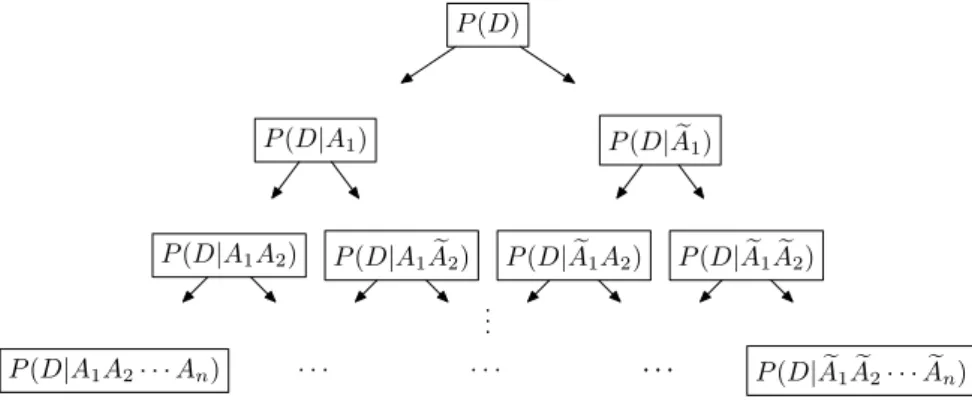
Fig. 2. Updating and integrating of evidential patterns in weights of evidence method. P (D)means the prior probability of mineral deposit occurrence;A1,A2,...,Anare different evidential patterns having positive correlations with mineral deposits andA˜1,A˜2,...,A˜n
are evidential patterns in contrary. The posterior probabilities are updated as the new evidence patterns are integrated; this figure can be compared with Fig. 1.
4.2 Generalized cascade process throughout mineralization and singularities
The similarity between the WofE method and multiplicative cascade models has been discussed in Cheng (2008), and a variant of WofE based on singularity was proposed as a novel approach for information integration. The posterior proba-bilities of mineral deposit occurrences are updated as new evidential patterns are put in (Fig. 2). Each evidential pattern represents the product of a certain geological process and the updated posterior probabilities represents its impact exerted on mineralization. Assuming mineralization as a singular event, the impacts caused by the participation of certain geo-logical processes should be accumulated nonlinearly so that singularities emerge. The updating of each evidential pattern and the relevant posterior probabilities is very similar to one cascade step and, therefore, we take the successive partic-ipating of new evidential patterns as a generalized cascade process. The nonlinear dynamics of interactions throughout mineralization can then be constructed by a generalized cas-cade model.
For an arbitrary evidential layer A, supposeAorA˜means presence or absence ofA, respectively. If we haven eviden-tial layers, then the total area can be divided into 2nsub-areas at last, marked by the different combinations of evidence. On each iteration of adding an evidence layer, the posterior prob-ability on each evidential combination will be distributed into two partitions. So this process can be regarded as a binary cascade process and the comparisons are shown in Fig. 3. As the figure shows, the singularity caused by the evidence layer A can be easily derived from Eq. (3) as:
α(A)=logP (A|D)/logP (A) (12)
The singularity of patternA˜ can be defined from the same procedures as:
αA˜=logPA˜|D/logPA˜. (13)
Equations (12) and (13) are important formulae to charac-terise the singularities of dynamical interactions between mi-neralization and certain geological processes. The formulae are based upon the assumption of mineralization as a singu-lar event and more detailed descriptions can be seen in Cheng (2008).
5 Cascade dynamics model of mineralization through multifractal simulation
Considering the posterior probability of mineralization due to a certain geological process as an indirect measurement of interaction between them, we can study the cascade dy-namics of mineralization from statistical points of view. The dispersion coefficientd, in an ordinary de Wijs model, could be regarded as a random variableD∗with a distribution of P (D∗=d)=P (D∗= −d)=1/2 (Agterberg, 2007a). Here the distribution of d should be identical to the distribution of an evidence which is denoted as Pe later on. The
fre-quency distribution of concentration values generated by a 1-D multiplicative cascade model is logbinomial, that is, the logarithmically transformed values have binomial distribu-tion (Agterberg, 2007a). So the logarithmic varianceσ2can be derived as:
η=(1+d)/(1−d)
σ2=nmaxPe(1−Pe)(lnη)2 (14)
wherenmaxmeans the maximum cascade division number.
WhenPe=1/2, Eq. (14) will follow intoσ2=nmax(lnη)2/4
corresponding to a simple de Wijs model (Agterberg, 2007a). The variance can be estimated from its relationship with the logarithmic variance:
s (lnx) s(x) ≈
d(lnx) dx
x= ¯x =1
¯
P
(
D
)
ρ
(
ǫ
n−1)
P
(
D
)
µ
(
ǫn
−1)
1
ǫ
n−1P
(
DA
)
/P
(
A
) =
P
(
D
|
A
)
µ
(
ǫn
)
/ǫ
=
ρ
(
ǫn
)
P
(
DA
)
µ
(
ǫ
n)
P
(
A
)
ǫ
ndecreasing scale
Fig. 3. Analogy between probabilities updated by an evidential layer and scale-invariant measures generated by multiplicative cascade process. This figure shows two consecutive iterations for demonstration. The prior probabilityP (D)is defined on the whole support 1, and one of its branches goes to posterior probabilityP (D|A)on patternA; this process is similar to the changing of measure fromµ(ǫn−1)to
µ(ǫn)as the scale decreases fromǫn−1toǫn, so does the fractal densityρ.
Equation (15) provides an approximation of variance for any random variablexwith meanx¯(cf. Agterberg et al., 1990). If the original concentration value in the multiplicative cascade model isξ, then the variance of final concentration values should be:
β2=ξ2σ2 (16)
whereβ2andσ2represent, respectively, variance and loga-rithmic variance of the final distribution. Therefore, we can deduce the maximum cascade division numbernmaxas long
as the dispersion coefficientd and logarithmic varianceσ2 or varianceβ2 are known. The parametersd andnmax are
crucial parameters for the multiplicative cascade model and they have been applied to simulate geochemical distribution (Agterberg, 2007a,b).
Consider a certain evidence layerA, the dispersion coeffi-cientdcan be estimated based on singularity calculated from Eqs. (12) and (13) as:
η=1+d
1−d =2
α(A)−α(A)˜.
(17) Equation (10) shows that the logits of posterior probabili-ties are the sum of weights determined by the combinations of all of the evidential patterns. The posterior probabilities stop updating after all the evidential layers are integrated suc-cessively and their results can be calculated from inversion of the logits. We suppose the posterior probabilities and their logits produced by WofE after integration of all available ev-idential layers are denoted asPf andLf, respectively. From the definition of logit function,Pf can be calculated as: Pf=eLf/(eLf+1). (18)
The standard deviation ofPf can be estimated by multi-plying the standard deviation ofLf byPf 1−Pf
(Fisher,
1971; Agterberg and Cheng, 2002). In order to estimate the standard deviation ofLf, firstly, variances of the weights can be estimated based on the asymptotic theory of discrete mul-tivariate analysis (Agterberg et al., 1990); these can be aug-mented by variances for missing data and added to the vari-ance of the prior logit, and then the result is an estimate of the standard deviation ofLf (Agterberg and Cheng, 2002). So the variance ofPf can be expressed as follows:
s2(Pf)≈Pf 1−Pfs(Lf) 2
(19) wherePfandLf are the post probabilities of mineral deposit occurrences and their logits, respectively;s2(Pf)ands2(Lf) are the variances ofPf andLf, respectively.
If the total number of evidential layers ism(m=4 in this example), that is, the number of involved geological pro-cesses ism, then 2m different patterns can be achieved by combination. The posterior probabilities would have 2m pos-sible values, so we can define a new random variablePF here and regardPf as the samples. Note that a binomial cascade model is used to distribute the posterior probabilities, so the expectation ofPF should be equal to the prior probability P0, which is considered as the original concentration. The
probability ofPF=Pf can be roughly estimated as the pro-portion of the pattern occupied by thePf in the total study area, thus, the variance ofPF can be estimated as follow: s2(PF)=
1 nt
2m X
f=1
nfs2(Pf) (20)
wherenf andnt are numbers of cells inside patterns occu-pied byPf and the total study area, respectively; mmeans the number of evidential layers. Suppose the final probabil-ities satisfy logbinomial distribution as the cascading result, the variance ofPF should be:
s2(PF)≈P02σ 2
Table 1.Statistics obtained from each of the four layers of binary maps (cf. Cheng, 2008).
Layer Pe α α(∼) 1α W+ s(W+) W− s(W−)
A 0.394 0.276 2.960 2.684 0.67 0.25 –0.97 0.47 B 0.568 0.084 3.657 3.573 0.57 0.23 –2.23 1.00 C 0.398 0.125 4.370 4.245 0.81 0.24 –1.68 0.67 E 0.194 0.391 3.465 3.074 1.00 0.31 –0.53 0.32
Average 0.388 0.219 3.613 3.394
whereP0means the prior probability of mineral deposit
oc-currences. Finally, we derive the following equation based on Eqs. (14), (20) and (21):
nmax=
s2(PF) P02Pe(1−Pe)(lnη)2
= 1
nt 2m X
f=1
nfPf2 1−Pf2s2 Lf P02Pe(1−Pe)(lnη)2
. (22)
wherent andnD mean numbers of units of the total study area and units of the mineral deposits, respectively. Equa-tion (22) can be used to estimate the maximum cascade divi-sion numbernmax.
6 Case study: validating the cascade dynamics model of mineralization
The nonlinear dynamics throughout mineralization were lacking research because of the difficulties to quantifying the interactions during mineralization. We propose a cascade dy-namics model to characterise mineralization based on statis-tical analysis of exploration data by WofE. Here, we will use a case study to demonstrate the usage and validate this model. The case study simulates mineral potential of gold deposits in the southwestern Nova Scotia, Canada. The simulation is im-plemented on the basis of the cascade dynamics model of mi-neralization. About 20 gold deposit occurrences are found in sedimentary rocks in the study area of about 7780 km2. The study area is gridded into 1×1 km2cells as GIS map layer and four deliberately designed evidence layers were used in Cheng (2008). Layers A and B represent binary patterns de-termined by optimum distance from anticline axes (2.5 km) and optimum distance from the contacts between Goldenville and Halifax formations (4 km), respectively. Layers C and E are two geochemical anomaly maps created by multifractal filter mapping of loadings of elements on two components derived via principle components analysis of geochemical concentrations of elements. In terms of geological back-grounds, layers A and B are, respectively, used to charac-terise the impacts to mineralization caused by the fold tec-tonics and metamorphosed sedimentary rocks which are sub-divided into the Goldenville and Halifax formations; layers C
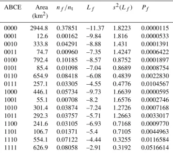
Table 2.Statistics obtained from combinations of the four layers of binary maps (cf. Cheng, 2008). The digits 0 and 1 correspond to the presence and absence of binary patterns, respectively.
ABCE Area nf/nt Lf s2(Lf) Pf
(km2)
0000 2944.8 0.37851 –11.37 1.8223 0.0000115 0001 12.6 0.00162 –9.84 1.816 0.0000533 0010 333.8 0.04291 –8.88 1.431 0.0001391 0011 74.7 0.00960 –7.35 1.4247 0.0006422 0100 792.4 0.10185 –8.57 0.8752 0.0001897 0101 85.4 0.01098 –7.04 0.8689 0.0008754 0110 654.9 0.08418 –6.08 0.4839 0.0022830 0111 257.1 0.03305 –4.55 0.4776 0.0104567 1000 446.1 0.05734 –9.73 1.6639 0.0000595 1001 55.1 0.00708 –8.2 1.6576 0.0002746 1010 301.4 0.03874 –7.24 1.2726 0.0007168 1011 292.3 0.03757 –5.71 1.2663 0.0033017 1100 241.6 0.03105 –6.93 0.7168 0.0009770 1101 106.7 0.01371 –5.4 0.7105 0.0044963 1110 554.1 0.07122 –4.44 0.3255 0.0116584 1111 626.9 0.08058 –2.91 0.3192 0.0516614
and D, respectively, correspond to the regional anomalies and local mineralization-associated anomalies favourable to mi-neralization which may originated from geochemical migra-tions in different scale (Cheng, 2008). More detailed descrip-tions of geological settings and datasets in this area can be found in Xu and Cheng (2001). For convenience, we only use some statistical results (Table 1) for our simulation from Cheng (2008) without discussing how to utilize the original data in the WofE method; more details about data processing and information integration can be found in Cheng (2008).
The value ofPe is set to the average probabilities of four
patterns (Pe=0.388); the dispersion coefficientsd are
0 0.01 0.02 0.03 0.04 0.05 0.06 0.07 0.08 0.09 0.1
0 100 200 300 400 500
Posterior probability of mineral potential
Sequence No.
Fig. 4. Multifractal simulation of posterior probabilities of min-eral deposit occurrences based on multiplicative cascade model; the original concentration was set to the prior probability of mineral de-posit occurrences, and the highest value was truncated below 0.1 in the figure. The sequence numbers only represent an arbitrary rank-ing of the simulated results, and the maximum sequence number is determined by the maximum cascade numbernmaxas 2nmax, that is,
512 in this example.
P0=20/7780=0.00257 was set as the original
concentra-tion and distributed to the final particoncentra-tions. Figure 4 shows the distribution of the posterior probabilities of mineral de-posit occurrences generated by multifractal simulation, and the highest value was truncated below 0.1. Known from Eq. (10), the WofE method can only generate posterior prob-abilities of mineral deposit occurrences whose amount is no more than the number of combinations by the evidential lay-ers. For example, the number of the values of posterior prob-abilities would not exceed 2mif there aremevidential layers involved. This sparse result provides little information for studying the distribution of mineral deposit occurrences. Al-though parts of statistical data are analysed from WofE, the respective mechanism represented by the cascade dynamics model is different from WofE. Thus, the distribution of the mineral potential generated by simulation is different from WofE. The number of possible results is associated to the maximum cascade division numbernmax, which reaches to
2nmax as Fig. 4 shows. However, the highest posterior proba-bilities which represent the most favourable areas to minera-lization should be reflected in the result of multifractal sim-ulation. From the simulation, we can see several peaks of values between 0.05 and 0.06 excluding one highest value; this is in accordance with the result of WofE. The multifrac-tal results can also be used to explain why singularities occur throughout mineralization, of which dynamical mechanism are still not clear.
7 Discussions and conclusions
Mineralization is a long process, so that it is impossible to ob-serve all the stages. However, nonlinear features have been discovered in the products of mineralization, from regional-scale of mineral deposits (Carlson, 1991; Agterberg et al., 1996), to micro-texture of minerals (Zhang et al., 2001; Zuo et al., 2009b), indicating that mineralization is a typical nonlinear process. In this article, we researched the inter-actions between mineralization and certain geological pro-cesses through statistical analysis of explorative data. Based on the proposition of taking mineralization as a singular event, the interactions can be regarded as generalized cas-cade dynamics and a cascas-cade model was constructed to sim-ulate the probabilities of mineral potential. Although the re-sult is from a statistical point of view, cascade dynamics may be the physical nature of interactions between mineralization and certain geological processes. The maximum cascade di-vision numbernmaxactually relies on the scale of the impacts
of certain geological processes. Some factors, like regional tectonics, could have large scale impacts on mineralization, while some factors, like migration of geochemical elements, have finer scale impacts.
The research established a simple theoretic model to learn nonlinear dynamics throughout mineralization, and the ex-ploration data are usually abundant to obtain so that the model is easy to set up. The multifractals generated by the cascade dynamics can be used to explain the singularities caused by mineralization. Unfortunately, the parameters in our model are also affected by conditional dependence of ge-ological data. From Eq. (22), we can find that conditional dependence between evidence layers will increase the vari-ance and lead to the larger nmax. However, if cascade
dy-namics were true in mineralization, then we could have some empirical values ofnmax, and actually this type ofnmaxhas
been discussed in the geochemical distributions (Agterberg, 2007a). The empirical values ofnmaxshould most probably
comes from the stochastic distribution of mineral deposits from some mature exploration area, where good training sets can be ensured. Thus, we can give a rough estimation of probabilities of mineralization from the multifractal simula-tion and improve the condisimula-tional independence limitasimula-tion of the weights of evidence method. It should be pointed out that the random generation of the dispersion coefficientd is also important to the cascade model, which was simplified to an ordinary De Wijs model in this paper. Agterberg (2007a) proposed random generation of the normal distribution in si-mulating geochemical distributions but the applications were still not enough, and it may need further research in the fu-ture.
Frits Agterberg. Thanks are due to two anonymous reviewers for their critical comments, and Ana Maria Tarquis for her careful review. The research was sponsored by a Distinguished Young Researcher Grant (40525009), a Strategic Research Grant (40638041), a General Research Grant (40972205) awarded by National Natural Science Foundation of China, a MOST Special Fund from the State Key Laboratory of Geological Processes and Mineral Resources, China University of Geosciences, a National High-tech R&D Program of China (2009AA06Z110), and an Outstanding Youth Teacher Fund from CUG (CUGQNL0939).
Edited by: J. Davidsen
Reviewed by: E. J. M. Carranza, A. M. Tarquis, and another anonymous referee
References
Agterberg, F.: New applications of the model of de Wijs in regional geochemistry, Math. Geol., 39, 1–25, doi:10.1007/s11004-006-9063-7, 2007a.
Agterberg, F. and Cheng, Q.: Conditional independence test for weights-of-evidence modelling, Natural Resources Research, 11, 249–255, doi:10.1023/A:1021193827501, 2002.
Agterberg, F., Bonham-Carter, G., and Wright, D.: Statistical pat-tern recognition for mineral exploration, in: Computer Applica-tions in Resource Estimation, edited by: Gall, G. and Merriam, D., Pergamon, Oxford, 1–21, 1990.
Agterberg, F., Cheng, Q., and Wright, D.: Fractal modelling of min-eral deposits, in: Proceedings of the International Symposium on the Application of Computers and Operations Research in the Minerals Industries, edited by: Elbrond, J. and Tang, X., Mon-treal, Canada, 43–53, 1996.
Agterberg, F. P.: Multifractal simulation of geochemical map pat-terns, J. China. Univ. Geosci., 12, 31–39, 2001.
Agterberg, F. P.: Mixtures of multiplicative cascade models in geochemistry, Nonlin. Processes Geophys., 14, 201–209, doi:10.5194/npg-14-201-2007, 2007b.
Bonham-Carter, G.: Geographic Information Systems for Geosci-entists: Modeling with GIS, Pergamon, Oxford, 1994.
Bonham-Carter, G., Agterberg, F., and Wright, D.: Integration of geological datasets for gold exploration in Nova Scotia, Pho-togramm. Eng. Rem. S., 54, 1585–1592, 1988.
Carlson, C. A.: Spatial distribution of ore deposits, Geology, 19, 111–114, 1991.
Carranza, E., Woldai, T., and Chikambwe, E.: Application of data-driven evidential belief functions to prospectivity mapping for aquamarine-bearing Pegmatites, Lundazi District, Zambia, Nat-ural Resources Research, 14, 47–63, doi:10.1007/s11053-005-4678-9, 2005.
Carranza, E., Hale, M., and Faassen, C.: Selection of coher-ent deposit-type locations and their application in data-driven mineral prospectivity mapping, Ore Geol. Rev., 33, 536–558, doi:10.1016/j.oregeorev.2007.07.001, 2008.
Cassard, D., Billa, M., Lambert, A., Picot, J.-C., Husson, Y., Lasserre, J.-L., and Delor, C.: Gold predictivity mapping in French Guiana using an expert-guided data-driven approach based on a regional-scale GIS, Ore Geol. Rev., 34, 471–500, doi:10.1016/j.oregeorev.2008.06.001, 2008.
Cheng, Q.: Comparison between two types of multifractal mod-elling, Math. Geol., 28, 1001–1015, doi:10.1007/BF02068586, 1996.
Cheng, Q.: Multifractal distribution of eigenvalues and eigenvectors from 2d multiplicative cascade multifractal fields, Math. Geol., 37, 915–927, doi:10.1007/s11004-005-9223-1, 2005.
Cheng, Q.: Singular mineralization processes and mineral resources quantitative prediction: new theories and methods, Earth Science Frontiers, 14, 42–53, 2007a (in Chinese).
Cheng, Q.: Mapping singularities with stream sediment geochem-ical data for prediction of undiscovered mineral deposits in Gejiu, Yunnan Province, China, Ore Geol. Rev., 32, 314–324, doi:10.1016/j.oregeorev.2006.10.002, 2007b.
Cheng, Q.: Non-linear theory and power-law models for informa-tion integrainforma-tion and mineral resources quantitative assessments, Math. Geosci., 40, 503–532, doi:10.1007/s11004-008-9172-6, 2008.
Cheng, Q. and Agterberg, F.: Fuzzy weights of evidence method and its application in mineral potential mapping, Natural Re-sources Research, 8, 27–35, doi:10.1023/A:1021677510649, 1999.
Cheng, Q. and Agterberg, F. P.: Singularity analysis of ore-mineral and toxic trace elements in stream sediments, Computat. Geosci., 35, 234–244, doi:10.1016/j.cageo.2008.02.034, 2009.
Cheng, Q., Agterberg, F., and Ballantyne, S.: The separation of geochemical anomalies from background by fractal meth-ods, J. Geochem. Explor., 51, 109–130, doi:10.1016/0375-6742(94)90013-2, 1994.
Cheng, Q., Agterberg, F., and Bonham-Carter, G.: Fractal pattern integration for mineral potential estimation, Natural Resources Research, 5, 117–130, doi:10.1007/BF02257585, 1996. Cheng, Q., Xu, Y., and Grunsky, E.: Multifractal power
spectrum-area method for geochemical anomaly separation, Natural Re-sources Research, 9, 43–51, 2000.
Cox, D. and Singer, D.: Mineral deposit models, US Geological Survey Bulletin 1693, 379, 143–161, 1986.
De Wijs, H. J.: Statistics of ore distribution, part I, Geologie en Mijnbouw, 13, 365–375, 1951.
Deidda, R.: Multifractal analysis and simulation of rainfall fields in space, Phys. Chem. Earth. Pt. B., 24, 73–78, doi:10.1016/S1464-1909(98)00014-8, 1999.
Evertsz, C. and Mandelbrot, B.: Multifractal Measures, in: Chaos and Fractals, edited by: Peitgen, H., Jiirgens, H., and Saupe, D., 922–953, Springer-Verlag, New York, 922–953, 1992.
Falconer, K.: Fractal Geometry: Mathematical Foundations and Applications, 2nd edn., Wiley, 2003.
Fisher, R.: The design of experiments, 9th edn., Macmillan, 1971. Ford, A. and Blenkinsop, T.: Combining fractal analysis of mineral
deposit clustering with weights of evidence to evaluate patterns of mineralization: Application to copper deposits of the Mount Isa Inlier, NW Queensland, Australia, Ore. Geol. Rev., 33, 435– 450, doi:10.1016/j.oregeorev.2007.01.004, 2008.
Lovejoy, S. and Schertzer, D.: Multifractals, cloud radiances and rain, J. Hydrol., 322, 59–88, doi:10.1016/j.jhydrol.2005.02.042, 2006.
Lovejoy, S., Schertzer, D., and Stanway, J.: Direct evi-dence of multifractal atmospheric cascades from planetary scales down to 1 km, Phys. Rev. Lett., 86, 5200–5203, doi:10.1103/PhysRevLett.86.5200, 2001.
Mandelbrot, B. B.: Fractals: Form, Chance, and Dimension, Free-man, San Francisco, 1977.
Mandelbrot, B. B.: The Fractal Geometry of Nature (updated and augmented edition), Freeman, New York, 1983.
Mandelbrot, B. B.: Multifractal measures, especially for the geophysicist, Pure Appl. Geophys., 131, 5–42, doi:10.1007/BF00874478, 1989.
Nyk¨anen, V.: Radial basis functional link nets used as a prospec-tivity mapping tool for orogenic gold deposits within the central Lapland greenstone belt, northern Fennoscandian shield, Natural Resources Research, 17, 29–48, doi:10.1007/s11053-008-9062-0, 2008.
Porwal, A., Carranza, E. J. M., and Hale, M.: Artificial neural net-works for mineral-potential mapping: A case study from Aravalli Province, western India, Natural Resources Research, 12, 155– 171, doi:10.1023/A:1025171803637, 2003.
Porwal, A., Carranza, E., and Hale, M.: Bayesian network classi-fiers for mineral potential mapping, Computat. Geosci., 32, 1–16, doi;10.1016/j.cageo.2005.03.018, 2006.
Raines, G.: Are fractal dimensions of the spatial distribution of min-eral deposits meaningful?, Natural Resources Research, 17, 87– 97, doi:10.1007/s11053-008-9067-8, 2008.
Sahoo, N. R. and Pandalai, H. S.: Integration of sparse geo-logic information in gold targeting using logistic regression anal-ysis in the Hutti–Maski Schist belt, Raichur, Karnataka, In-dia – a case study, Natural Resources Research, 8, 233–250, doi:10.1023/A:1021698115192, 1999.
Schertzer, D. and Lovejoy, S.: Physical modelling and anal-ysis of rain and clouds by anisotropic scaling of multi-plicative processes, J. Geophys. Res., 92(D8), 9693–9714, doi:10.1029/JD092iD08p09693, 1987.
Schertzer, D. and Lovejoy, S.: Nonlinear geodynamical variabil-ity: multiple singularities, universality and observables, in: Non-linear Variability in Geophysics, edited by: Schertzer, D. and Lovejoy, S., Kluwer Academic Publishers, Netherlands, 41–82, 1991.
Singer, D. and Kouda, R.: Application of a feedforward neural net-work in the search for kuroko deposits in the Hokuroku District, Japan, Math. Geol., 28, 1017–1023, doi:10.1007/BF02068587, 1996.
Turcotte, D.: Fractals and Chaos in Geology and Geophysics, 2nd edn., Cambridge University Press, Cambridge, 1996.
Xu, Y. and Cheng, Q.: A fractal filtering technique for processing regional geochemical maps for mineral exploration, Geochem.-Explor. Env. A., 1(2), 147–156, 2001.
Yu, C., Tang, Y., Shi, P., and Deng, B. L.: The Dynamic Sys-tem of Endogenic Ore Formation in Gejiu Tin-Polymetallica Ore Region, Yunnan Province, China University of Geosciences, Wuhan, 1988.
Zhang, S., Cheng, Q., and Chen, Z.: Omnibus weights of evidence method implemented in GeoDAS GIS for information extraction and integration, J. China, Univ. Geosci., 19, 404–409, 2008. Zhang, Z., Mao, H., and Cheng, Q.: Fractal geometry of
ele-ment distribution on mineral surfaces, Math. Geol., 33, 217–228, doi:10.1023/A:1007587318807, 2001.
Zuo, R., Cheng, Q., Agterberg, F., and Xia, Q.: Application of singularity mapping technique to identify local anomalies using stream sediment geochemical data, a case study from Gangdese, Tibet, western China, J. Geochem. Explor., 101, 225– 235, doi:10.1016/j.gexplo.2008.08.003, 2009a.