SIMULATION MODEL BASED ON IACS DATA; ALTERNATIVE APPROACH TO ANALYSE SECTORAL INCOME RISK IN AGRICULTURE

(1)

Review of Agricultural and Applied Economics The Successor of the Acta Oeconomica et Informatica ISSN 1336-9261, XIX (Number 1, 2016): 56–64

doi:10.15414/raae/2016.19.01.56-64

RAAE

REGULAR ARTICLE

SIMULATION MODEL BASED ON IACS DATA; ALTERNATIVE APPROACH TO

ANALYSE SECTORAL INCOME RISK IN AGRICULTURE

Jaka ZGAJNAR

Address:

University of Ljubljana, Biotechnical faculty, Department of Animal Science, Groblje 3, SI 1230 Domzale, phone: +386-31-343-507. E-mail: jaka.zgajnar@bf.uni-lj.si

ABSTRACT

We develop a static simulation model to analyse income losses and income risks at aggregated agriculture sector level. Our empirical case study is based on farm level records for direct payments claims (IACS data) and covers the period 2010–2011. Using Monte Carlo simulations, we investigate the impact of different levels of risk on income trends. Results show that 80% of farms are extremely dependent on direct payments. Farm production types highly supported by direct payments consequentially fall into the low-risk group. Results show that a significant share of income loss at sector level is carried by small farms (by economic class). Average probability of larger losses at the sector level ranges between 2% and 64%. Our results also indicate that larger farms often have better risk-return ratios and thus face lower relative income risks.

Keywords: income stabilisation tool, risk analysis, direct payments, MCS, EU

JEL: R52, R58, H41

INTRODUCTION

Understanding the economic implications and risks of income variability does not only represent an important task for risk management, but is also very important in assessing and developing new risk management strategies and tools. Stable farming is a fundamental tenet for each agricultural holding. In the last decade, the issues of risk and possibilities of income risk stabilisation have gained on importance for farmers, policy-makers and other stakeholders. This is not only due to increased production risk caused, for example, by diseases and climate events, but also due to the growing liberalisation and globalisation of agricultural markets, which is reflected in increased volatility of input and output prices (Meuwissen, Van Asseldonk and Huirne, 2008a).

Liesivaara, Myyrä and Jaakkola (2012) find that a major part of income variability comes from price volatility and not from yield variation. Tangermann (2011)stresses that for the first time since the 1970’s, high

volatility in agricultural markets has become highly significant, and this trend may continue (Mary, Santini and Boulanger, 2013b).

Additionally, changes introduced into or planned for the EU Common Agricultural Policy (CAP) show that farmers will have to assume the responsibility for managing the risk that was formerly mitigated by market and price support policy (Janowicz-Lomott and Lyskawa, 2014). Hence, parallel with the global financial crisis, all this has amplified the interest for risk management in agriculture, indicating the need for proper income risk management strategies and tools, supported by appropriate policy measures.

Many studies show that risk management has become an important new agricultural policy concept both in OECD and non-OECD countries (e.g., Meuwissen, Van

Asseldonk and Huirne, 2008; Anton, 2008; OECD, 2011; Meuwissen et al., 2011; Turvey, 2012; Mary, Santini and Boulanger, 2013b; Finger and El Benni, 2014a; Janowicz-Lomott and Lyskawa, 2014).

Janowicz-Lomott and Lyskawa (2014) see option that income stabilisation fund take over the role of direct payments in the EU.

There are several studies dealing with the possibility of implementing the Income Stabilisation Tool (IST) to tackle income volatility issues in the EU (e.g., Meuwissen et al., 2011; Liesivaara, Myyrä and Jaakkola, 2012; Mary, Mishra and Gomez Y Paloma, 2013a; Mary, Santini and Boulanger, 2013b; Finger and El Benni, 2014a; Finger and El Benni, 2014b). Recently agricultural policy and agricultural economists in the European Union have revealed the possibility of budgetary support and initiatives for the development of a carefully tailored set of policy measures. It is a policy that is already being widely implemented in other developed countries, particularly the USA and Canada. Whole-farm income is arguably the best measure of agricultural holdings’ welfare and therefore also appeals to policy makers (Meuwissen et al., 2011).

(2)

Setting new agricultural policies or measures to support farms requires monitoring income stability and variability as indicators of farm production conditions (Zgajnar, 2013). In many countries, the intention to analyse income risks and subsequently search for solutions, stumbles upon the problem of insufficient data. Since long and consistent series of farm-level data are usually not available, analyses often use aggregated data. While there are aggregation biases in risk analysis at farm level (see Finger, 2012b), aggregation is especially applicable for preliminary analyses in a comprehensive income risk approach at the regional or national level. Namely, risk management at the agricultural holding level is very demanding from the information viewpoint (Anton et al., 2011). It requires information about different risk sources at the level of each agricultural holding. The availability of historical farm-level data is a major constraint in the analysis of risk exposure of individual farms (OECD, 2011).

There are many studies where FADN data were applied to analyse income risks and stabilisation tools at the farm and sector level (e.g., dell’ Aquila and Camino,

2012; Liesivaara, Myyrä and Jaakkola, 2012; Mary, Santini and Boulanger, 2013b; Finger and El Benni, 2014b; Meuwissen, Van Asseldonk and Huirne, 2008a; Vrolijk and Poppe, 2008). In most cases the aim is not to analyse income losses at a particular farm (as an insurance scheme), but to analyse the situation on a sample of farms. Different approaches to analysing income risk issues and other datasets than FADN can also be found in the literature. Turvey (2012), for example, applied a mathematical programming model to investigate different income insurance schemes in the USA and Canada. He used different data for yield distributions and price volatilities, obtained from Statistics Canada and the Central market. An approach to cross-sectoral comparison of income risk, in which the concept of ‘Weather Value at Risk’ is extended in order to describe and compare sectoral income risks due to climate change, is presented by Prettenthaler, Köberl and Bird (2015). This concept was primarily developed to measure the economic risks resulting from current weather fluctuations. In their research they compared sectoral income risks in agriculture and tourism.

We develop a static simulation model to analyse income risk at sector level. The main idea is to apply a bottom-up approach, meaning that available farm-level information is utilised to estimate the income risk situation for different production groups of farms and for the sector as a whole. The main assumption is that there are no bookkeeping data available for the farm level, but that information regarding main production activities is available. For this purpose, as opposed to other studies based on FADN or bookkeeping data, the Integrated Administration and Control System (IACS) database was applied. This database allows for the acquisition of information on the physical production structure for each agricultural holding in a given period. To our knowledge, this is the first such attempt to use this database, which is available for all EU countries. We followed a three-step procedure in order to derive different distributions of farms income and to calculate income risk.

The primary objective of the paper is to present and discuss the suggested simulation approach using the IACS database as an adequate approach to describing and comparing income risks at the sector level, and to determine whether it is a useful tool to present preliminary risk information to stakeholders and decision makers. The second purpose is to acquire preliminary numbers regarding income risk. In that context, particular emphasis is put on probability evaluations and the identification of potential beneficiary groups among farmers, comparable to, for example, Zgajnar (2013), where the approach was only applied to the pig sector, or Zgajnar and Kavcic (2013), where the dairy sector income risk issues were elaborated in detail.

Database and estimation of the economic situation at the farm level

The developed model is based on real data for all farms that applied for subsidies in the years 2010 and 2011. Thus, the main information for each agricultural holding represents its physical production in a particular year. These are annual data derived from subsidy claims (IACS) collected by the Slovenian Payment Agency. For the purposes of this study we considered data for CAP 1st pillar payments and Less Favoured Areas payments (LFA). In this way, we acquired information regarding the farms’ main production activities and the extent to which they were practiced on a particular farm. Based on this information we reconstructed production plans for each agricultural holding in the database. The main benefit of the IACS database is that it enables acquiring some information on all farms applying for direct payments, regardless of whether they keep records. Consequently almost all agricultural holdings in the sector could be analysed.

From the IACS database, one can infer the farming type and approximately estimate production volumes, yielding some information about all agricultural holdings in a particular agricultural sector without the accounting data needed for detailed analyses of income risk (Liesivaara, Myyrä and Jaakkola, 2012; Finger and El

Benni, 2014b). This is also the main disadvantage of the approach presented in this paper. Namely, we chose a rather robust method of estimating monetary values. The resulting figures are regarded as proxies for income on each farm. In addition, the main challenge was the estimation of achieved revenues, gross margins and incomes for each agricultural holding, to imitate income risk.

(3)

RAAE / Zgajnar, 2016: 19 (1) 56-64, doi: 10.15414/raae.2016.19.01.56-64

58 from internal data sources prepared by the Agricultural Institute of Slovenia. Further SOs at the agricultural holding level were calculated based on the methodology proposed by the European Commission (Rednak, 2012). The main assumption in our analysis was that the production plan remains fixed and that farmers cannot add additional activities to the production plan in a particular year (state of nature). To overcome this strong assumption, the dynamic stochastic paradigm should be applied in further steps, as is done, for example, by Mary, Santini and Boulanger (2013b).

The IACS database for Slovenia includes 59,629 agricultural holdings (Table 1), mainly small scale-farms with a diversified enterprise composition. They are further divided into 21 farm types. This classification was constructed by Rednak (2012) according to the structure of total SOs for each agricultural holding, taking into account the contribution of the main production activities. To enable analysis of differences within each production type, farms were subdivided into 13 economic classes. According to the estimated standard output (SO) without direct payments, economic classes range up to 3 million euros of annual turnover. The number of farms with specific production types and in different economic classes is shown in Table 1.

The crucial drawback of this approach for risk analysis is that for all farms analysed in the model, the same average productivity and average market prices are assumed. To decrease the influence of this bias, additional indices to adjust SOs for crucial activities were calculated. An example is the SO that was adjusted for crop activities (e.g., wheat, barley and maize). In this case the total arable land of each agricultural holding was considered to influence the efficiency of production – economy of scale. Smaller areas of arable land per farm (smaller than the average national production amount significant for a particular sector) also result in lower SOs, and vice versa. In all examples five different indices were considered, ranging from –20% to +20%. A similar example is adjusting the SOs for milking cows, where the deviation from average milk production during lactation and average milk production per farm (calculated as the farm milk quota divided by the number of dairy cows in the herd) is considered. Indices range between –30% and +30%. A similar approach was also applied to adjusting fixed costs (FC) at the farm level, where the main indicator was the total utilized agricultural area. Coefficients range between –25% and +15% of total estimated fixed costs at the farm level.

To obtain total average revenues of agricultural holdings, SOs were increased by eligible subsidies from the first and second pillar of the CAP. This was done based on information derived from the IACS dataset. Since most subsidies are decoupled, it was not possible to directly estimate revenues at the level of a particular activity in the production plan, but at the farm level. This was also considered when defining costs. Namely, variable and fixed costs are calculated in the model as a relative share of the SO for each activity. Both were based on a historical data-set prepared by analytical model calculations (AIS, 2013) and additional expert estimates.

Simulation model for evaluating risk at farm level

To assess the effect of different normal and catastrophic risks that agricultural holdings might face, a complex static simulation model reflecting possible income losses at farm level was developed. Simulations are performed based on Monte Carlo Simulation (MCS), which is often used for studying different systems involving uncertainty. It relies on random sampling of values for uncertain variables included in simulation models based on Latin Hypercube sampling.

MCS is particularly suitable for simulating the effects of stochastic variables generating production effects (random function) based on input risks like change of variable costs (random variable). The risk of input units is defined by a probability distribution function and simulated with random number generators. Literature review reveals that probability distributions are most commonly defined based on (i) time-series data (if available) and (ii) literature review, seeking parallels with other studies; there is also increasing application of (iii) analytical distributions.

Due to the preliminary nature of the model and to keep its simplicity at this development stage, common triangular uncertain distributions were assumed for all uncertain variables addressing farming activities. These distributions are defined by minimum (x), maximum (z) and most likely (y) values which were defined according to deflated historical data (AIS, 2013). In this manner, the changes over time of SOs and variable costs were determined for each particular activity. In the current version of the tool, over 200 random variables were defined for production units.

The literature shows that in most cases when analyses are based on this type of approach and average values, values of extreme events can be problematic. They are usually underestimated, and this can be especially problematic in the analysis of income risk, which also captures extreme events. For example, Turvey (2012) in his analysis increased the standard deviation by 75% to overcome the issue of lower yield variability, since estimates were based on the provincial averages. So when time series data are used to define probability distributions, it is important to take a slightly lower value than the actual minimum and a slightly higher value than the actual maximum.

Description of the simulation model

The simulation model simulating the achieved income (I) per agricultural holding (f) in different states of nature (j) can be defined as follows in Eq. (1) till Eq. (7).

f f fj

fj GM FC g

I   (1)







 n

i ij

fj GM SUB

GM

1

(2)

j i i j i i i

ij SOeas SOPbss

GM   (3)

) , , (

s s s s i i i

i Triangular x y z

(4)

Table 1 Number of agricultural holdings divided by production type and economic classes (taken from Rednak (2012))

Type Economic classes (SO, 1,000 EUR) _∑

up

to

2

–

4

-

8

–

15

-

25

-

50

-

100

-

250

-

500

-

750

-

1

,000

1,

000

-

1,

500

1,

500

-

3,

000

othe

r

Code 1 2 3 4 5 6 7 8 9 10 11 12 13 14

11 1,471 1,336 960 309 121 93 25 6 2 1 0 1 2 0 4,327 12 0 0 0 2 4 11 14 40 17 0 0 1 1 0 90 13 400 410 175 27 9 1 3 1 0 0 0 0 0 0 1,026 14 3,106 1,918 654 112 64 42 10 3 1 0 0 0 0 0 5,910 P2 12 39 39 64 40 56 17 16 1 0 0 0 0 0 284 31 118 297 445 336 224 122 28 5 2 1 1 1 1 0 1,581 32 48 151 240 233 163 145 107 42 6 1 1 1 2 0 1,140 33 1 32 68 53 11 8 0 0 0 0 0 0 0 0 173 34 19 78 156 155 84 69 18 3 0 0 0 0 1 1 584 41 0 11 105 548 1,210 2,248 1,328 435 18 2 0 0 3 1 5,909 421 146 553 1,013 526 117 31 5 0 0 0 0 0 0 0 2,391 422 306 1,446 2,641 1,983 693 291 60 15 0 1 0 0 0 0 7,436 43 132 797 2,197 1,664 653 269 72 10 1 0 0 0 0 0 5,795 44 333 773 786 322 102 57 12 4 0 0 0 0 0 0 2,389 45 165 586 808 426 122 47 12 3 0 0 0 0 0 0 2,169 51 7 16 31 55 71 154 114 43 4 0 0 0 1 2 498 52 2 8 10 2 8 15 49 114 20 7 0 1 2 2 240 53 16 22 17 10 5 3 4 8 3 0 0 0 0 0 88 P6 1,017 2,031 1,328 384 97 75 37 7 1 0 0 0 0 0 4,977 P7 89 646 1,298 895 318 213 68 30 6 1 0 0 0 0 3,564 P8 621 1,695 3,335 2,121 671 415 147 44 5 0 1 2 0 1 9,058

∑ 8,009 12,845 16,306 10,227 4,787 4,365 2,130 829 87 14 3 7 13 7 59,629

Note:Legend for farming type: 11-Agriculture; 12-Hop; 13-Agriculture mixed; 14-Forage production; P2-Vegetables; 31-Vineyards; 32-Fruits; 33-Olive plantations; 34-Permanent crop mixed; 41-Dairy production; 421-Suckler cows; 422-Beef; 43-Cattle mixed; 44-Small ruminants; 45-Grazing animals mixed; 51-Pigs; 52-Poultry; 53-Granivores mixed; P6-Crop mixed; P7-Livestock mixed; P8-Mixed farming

) , , (

ss ss ss

ss i i i

i Triangularcx cy cz

b  (5)

1 2 3 1 2 3

min ( , , ; _s, _s , _s )

sBino al s s s p p p (6)

) , ; , (

minal ss₁ ss₂ p_ss₁ p_ss₂ Bino

ss (7)

Where represents fixed costs per farm (f), which are presumed to be fixed across different states of nature. However, special calibrating coefficients are added to adjust fixed costs per farm within a particular farming type, reflecting the size of total tillage area. � (Eq. (2)) represents the total gross margin achieved at the agricultural holding level, which is the sum of all activities’ gross margins � , with different values between states of nature . �� includes all subsidies from the first pillar, including historical payments, as well as LFA payments. All subsidies are presumed to remain constant throughout the simulation process. � is an index generated from the triangular distribution to adjust the � , of activity , for each state of nature , in respect to the selected scenario �. is a static coefficient introduced to adjust the average � of activity to particular farm characteristics (e.g., crop/maize production). Variable

costs are calculated as a percentage of � , and �� is an index generated from the triangular distribution to adjust the variable costs for each state of nature, given each selected scenario (��).

Within the simulation process, different scenarios representing different levels and types of risk (e.g., normal/catastrophic, correlated/uncorrelated, systemic) at the level of SOs and variable costs (VC) are presumed. Two uncertain variables (� and ��) are included in the model to randomly select a scenario which is in place in a particular state of nature for the SO and VC per analysed agricultural holding. In both cases, a common binomial distribution with defined probabilities of occurrence was assumed (Eq. 6 and Eq. 7). Consequently, five uncertain coefficients were defined for each parameter of activities’ triangular distribution in the model: three for SO scenarios (s) and two for variable costs scenarios (ss).

(5)

60 widened. The third scenario for SOs and second scenario for variable costs anticipate catastrophic – extreme events, with significantly higher frequencies of very bad, as well as very good outcomes. In most cases this means that the outcome (revenue – in our case expressed as SO) might also be zero or close to zero, while it is less likely that the outcome will be very good. Just the opposite holds for the uncertainty indices for variable costs.

Which scenario is selected in a particular state of nature depends on a discrete uncertain variable, based on the binominal distribution. In the proposed analysis, simulation includes 5,000 states of nature, which means that outputs for each activity and agricultural holding were calculated for 5,000 randomly sampled values.

RESULTS AND DISCUSSION

The paper presents aggregate results for all 21 farm types within Slovenian agriculture (Table 1). Due to space limitations, only aggregate results are presented. To provide insight into the shares and importance of particular farm types, first the entire agricultural sector is briefly presented, based on SOs, incomes and direct payments. In addition to the magnitude of income risk, measured as riskiness of a particular sector, probabilities of greater income losses are also presented. In all cases, estimates are based on aggregate results for all farms within a group (e.g., economic class – EC).

With analysis at the sector level, we tried to obtain information regarding the importance of income risk in Slovenia and the sectors that demand special attention. In the context of managing income risks, it is important to know how many such agricultural holdings there are and what their impact is at the aggregate level. In Slovenia, based on our estimates, the economic size of not more than 4,000 euros SO, is achieved by more than a third of farms. More than 44% of agricultural holdings achieve between 4,000 and 15,000 euros of SO, while close to 80% of agricultural holdings annually achieve less than 15,000 euros in total. Most generate an income that is less than the total value of received direct payments, which are an important factor of income stability (Severini and Tantari, 2013).

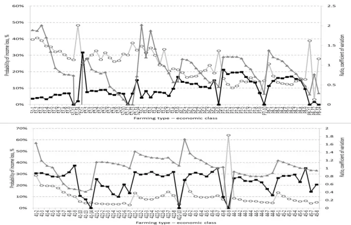
Regarding the estimated SOs, the most important sector is dairy, followed by beef and mixed farming. Grazing livestock accounts for more than 50% of estimated total income. Other mixed production types together represent less than one fifth of aggregate income, while overall crop production exhibits a relatively low share in aggregate income due to the large proportion of final realization through livestock. Since CAP measures are generally an important income source for EU farms and to outline the situation in Slovenian agriculture, part of this analysis was also to compare the level of budgetary support and estimated income realisation (Fig. 1). This gives additional information about possible influences on income stabilisation.

The analysis showed that direct payments have a significant impact on the severity of income risk at the individual holding level. More detailed analysis at the level of agricultural holdings within each economic size

class shows that four-fifths of farms are extremely dependent on budgetary payments (even greater than or equal to the indicator of income at the same holding). Dependency was measured as the ratio between budgetary support and expected income and is especially significant for groups of farms classified as agriculture mixed (13), grazing livestock without large dairy farms (41, 421, 422, 43, 44, 45), as well as for all mixed types of farms (P6, P7 and P8). In other production types, mainly the small-scale farms in lower economic classes are highly dependent on budgetary payments. As Figure 1 shows, the ratio between income and direct payments is relatively wide. This is a surprising result, especially for a sector that is not directly entitled to direct payments. This wide ratio can be explained by low incomes typical of this sector, since revenues rarely cover production costs (particularly pronounced for small ECs), and since budgetary payments are in the form of (decoupled) regional payments. However, farms with such payments are relatively few. A similar effect can also be seen in production type 53-granivores mixed. Though these results are important for understanding the riskiness for the analysed group of farms and probabilities of larger income losses, they are not further presented due to space constraints.

The results for income risk at the aggregate level for each production type and economic size are presented in Figure 1. It is evident that the average probability of income loss greater than 30% changes between groups of farms within different production types and economic sizes. The average probability of greater losses ranges between 2% and 64%, while the 20%, picks on possible indemnification. Namely, only losses above this curve should be considered when estimating eventual indemnities. On average, the probability of greater losses at the sector level is 21%. Compared to the study of

Liesivaara, Myyrä and Jaakkola (2012) in a case of Finnish farms, this is relatively low. However this may be because direct payments in our analysis are considered as fixed and certain, and therefore reflected in reduced income volatility.

(6)

Note: (Farming type – economic class); 11-Agriculture; 12-Hop; 13-Agriculture mixed; 14-Forage production; P2-Vegetables; 31-Vineyards; 32-Fruits; 33-Olive plantations; 34-Permanent crop mixed; 41-Dairy production; 421-Suckler cows; 422-Beef; 43-Cattle mixed; 44-Small ruminants; 45-Grazing animals mixed; 51-Pigs; 52-Poultry; 53-Granivores mixed; P6-Crop mixed; P7-Livestock mixed; P8-Mixed farming

(7)

62 In this respect, differences between farms within each economic class are also important. They are measured with coefficients of variation (CV). With some minor exceptions, larger discrepancies occur in those groups where the probability of larger losses is relatively low. Of course, the number of farms in each EC group must also be considered (Table 1). From Figure 1 it is apparent that for sectors with a relatively low likelihood of large losses there is a significant trend of large differences (CV) between agricultural holdings within the group. Typical examples are agriculture mixed (13), forage production (14), suckler cows (421), beef (422) and small ruminants (44). This indicates that some farms within these groups are also faced with a relatively high income risk. By contrast, for farms within vegetables (P2), vineyards (31), pigs (51) and poultry (52), it is obvious that the difference between farms is much lower, indicating that a relatively large share of holdings in these groups is confronted with high income risk.

We further divided the analysed farm types into three groups according to riskiness of income: high-risk, medium-risk and low-risk (Fig. 2). The average frequency of income loss greater than 30% of the average income is considered as the main indicator of the level of income risk. If the average frequency is greater than 0.3, the farming type is assigned to the high-risk group. Probabilities between 0.1 and 0.3 define the second – medium-risk group, and probabilities lower than 0.1 define the third – low-risk farming group type.

Legend: (Farming type – economic class); 11-Agriculture; 12-Hop; 13-Agriculture mixed; 14-Forage production; P2-Vegetables; 31-Vineyards; 32-Fruits; 33-Olive plantations; 34-Permanent crop mixed; 41-Dairy production; 421-Suckler cows; 422-Beef; 43-Cattle mixed; 44-Small ruminants; 45-Grazing animals mixed; 51-Pigs; 52-Poultry; 53-Granivores mixed; P6-Crop mixed; P7-Livestock mixed; P8-Mixed farming

Figure 2 Riskiness by production type

The average frequency is calculated as a weighted average for each group that takes into consideration the number of agricultural holdings within each group of economic classes. The value therefore represents a farming type. Of course, within each group of farming types, there are differences between economic classes (EC) (Fig. 1). In the preliminary results, there is no notable trend between groups of farming type. However, it has to be noted that the coefficients of variation in some ECs

exceed 0.6. Further analysis showed that the higher the probability of income loss (greater than 30% of average income), the lower the coefficient of variation within the economic class.

Model results in Figure 2 show that the high-risk group contains hop production, permanent crops production without olives and breeding granivores including pigs. The medium-risk group contains dairy, specialised and mixed agriculture and olive plantations. Low-risk farm production types turned out to be farms with grazing animals specialised in meat and forage production. In these farming activities, direct payments are a key income-stabilising factor, as also revealed by Figure 1. This is especially significant for small-scale agricultural holdings (regarding SO), as well as in some other farming types, classified in the other two groups.

CONCLUSION

Analysing income risks that groups of agricultural holdings face significantly differs from the approach for estimating actual losses of income on a particular holding. Using the IACS database as presented in this paper seems to be pragmatic and applicable for systematic comprehensive analyses of income risks at sector level. Such information is needed to obtain rough estimates of the income situation at sector level in agriculture, especially for policy makers deciding on the introduction, design and development of an income-stabilising scheme or tool.

Based on the presented results, we can conclude that the developed simulation model enables the study of income risk issues and probabilities of income losses at the level of different groups of farms, as well as at the level of entire sector. In further research, estimations and analyses of potential indemnities at the level of beneficiary groups of farms could also be done with the model.

The applied bottom-up approach, where the main information for each agricultural holding is gathered from direct payment claims (IACS database), enables the robust reconstruction of the production plan on each analysed agricultural holding. Except for the amount of direct payments, there are no other microeconomic data available at farm level. Due to this strong assumption, the presented approach has some limitations for income risk analyses. In this regard the most critical component is the estimation of standard outputs, variable costs and gross margins for each activity and agricultural holding. In most cases it is based on national averages and consequentially a large part of the variability is lost. For example, Finger (2012b) found that with increased aggregation, variability in crop yield could change up to 2.38 times. Similarly,

Turvey (2012) stresses that, on average, individual farm yields ranged from about 66% to 125% higher than an average yield metric.

(8)

In further model development it is therefore necessary to include additional information from other available data sources at the micro level (e.g., FADN) and in this way create a meta-data-base. Such information could be included as an additional calibration index, for example per region, technology, farm size. So, for different groups of agricultural holdings as well as for activities, more precise random distributions could also be defined. Since correlations (price-yield or yield-yield) are not considered (assumed to be zero), it is expected that the income risk is overestimated in some farm cases, because the natural hedge is not taken into consideration. However, considering the findings by Finger (2012a) that at the farm level much smaller price-yield correlations could be observed than at the aggregate level, the bias is probably similar in our case; namely, due to the presented approach, only correlations at the national level could be considered. This could also be a subsequent step of this research when analysing FADN data.

Results of the case study allow for the conclusion that the high income risks that could be managed with appropriate policy measures in Slovenia are a problem for a relatively small number of agricultural holdings. These holdings derive a large share of their income from market production or are rather narrowly specialized. In such cases, holdings can be faced with even higher income risks than reflected by model results at the particular sector level. However, it is also important to consider the natural hedge at the farm level due to the negative correlation between prices and yield levels (Finger, 2012a). Additionally, Finger (2012b) found that increasing crop acreage (larger farms) leads to decreasing crop yield variability. So in crop production this might also be a risk-reducing strategy.

According to Anton (2008), agricultural support policies have a significant role in risk management, even if not directly oriented towards reducing risk; our research confirmed this finding. Model results show that direct payments have a significant influence on income risk, and especially on probabilities of larger losses. For sectors that are relatively well supported with CAP measures, the probability of larger income risk is reduced and these farms therefore enter the low-risk group. Results show that there are significant differences between production types, as well as economic classes within these groups. For sectors with a relatively low likelihood of larger losses, there is a significant trend of big differences occurring between agricultural holdings within the group. Our results are in line with the findings of Finger and El Benni (2014a), who stress that larger farms (higher EC) face lower (relative) income risks than smaller farms with low levels of expected incomes and are also less likely to get indemnification from such a scheme (IST).

REFERENCES

AIS, 2013. Model calculations. Agricultural Institute of Slovenia. Ljubljana, Slovenia. Available at:

http://www.kis.si/pls/kis/!kis.web?m=177&j=SI>

ANTON, J. 2008. Agricultural policies and risk management: a holistic approach. In: Berg E., Huirne R., Majewski E., Meuwissen M. (eds.). Income stabilisation

issues in a changing agricultural world: policy and tools.

Warsaw, Poland: Wies Jutra. p. 15–28. ISBN 83-89503-65-4

dell’ AQUILA, C. and CAMINO, O. 2012. Stabilization

of farm income in the new risk management policy of the EU: a preliminary assessment for Italy through FADN data. In: 126th EAAE Seminar New challenges for EU agricultural sector and rural areas. Which role for public policy?, in June in Capri, Italy. p. 16.

FINGER, R. and El BENNI, N. 2014a. A Note on the Effects of the Income Stabilisation Tool on Income Inequality in Agriculture. Journal of Agricultural Economics 65(3), 739–745. doi: 10.1111/1477-9552.12069

FINGER, R. and El BENNI, N. 2014b. Alternative Specifications of reference Income Levels in the Income Stabilization Tool. In: Zopounidis, C., KALOGERAS, N., Mattas, K., van Dijk, G., Baourakis, G. (eds.).

Agricultural Cooperative management and Policy. New Robust, Reliable and Coherent Modelling Tools.

Switzerland: Springer International Publishing Switzerland. p. 65–85. ISBN: 978-3-319-06634-9 (Print) FINGER, R. 2012a. How strong is the “natural hedge”? The effects of crop acreage and aggregation levels. In:

Price volatility and Farm Income Stabilisation, Modelling Outcomes and Assessing Market and Policy Based Response, 123rd_{EAAE Seminar}_{, in February in Dublin. p.}

16.

FINGER, R. 2012b. Biases in Farm-Level Yield Risk Analysis due to Data Aggregation. German journal of agricultural economics 61(1), 30–43.

JANOWICZ-LOMOTT, M. and LYSKAWA, K. 2014. The new instruments of risk management in agriculture in the European Union. Procedia Economics and Finance 9: 321–330. doi:10.1016/S2212-5671(14)00033-1

LIESIVAARA, P., MYYRÄ, S. and JAAKKOLA, A. 2012. Feasibility of the Income Stabilisation Tool in Finland. In: Price volatility and Farm Income Stabilisation, Modelling Outcomes and Assessing Market and Policy Based Response, 123rd_{EAAE Seminar}_{, in}

February in Dublin. p. 12.

MARY, S., MISHRA, A. and GOMEZ Y PALOMA, S. (2013a). An impact assessment of EU's CAP income stabilisation payments. In: Agricultural & Applied

Economics Association’s 2013 AAEA & CAES Joint

Annual Meeting, in August in Washington, DC. p. 12. MARY, S., SANTINI, F. and BOULANGER, P. 2013b. An Ex-Ante Assessment of CAP Income Stabilisation Payments Using a Farm Household Model. In: 87th Annual Conference of the Agricultural Economics Society, in April in Warwick, UK. p. 13.

MEUWISSEN, M.P.M., MAJEWSKI, E., BERG, E., POPPE, E. and HUIRNE, R.B.M. 2008b. Introduction to income stabilisation issues in a changing agricultural world. In: Berg, E., Huirne, R., Majewski, E., Meuwissen, M. (ed.). Income stabilisation issues in a changing agricultural world: policy and tools. Warsaw, Poland: Wies Jutra. p. 7–12. ISBN 83-89503-65-4

MEUWISSEN, M.P.M., VAN ASSELDONK, M.,

KYÖSTI, P., HARDAKER, B., HUIRNE, R. 2011.

(9)

64

Uncertainty, Challenges for Agriculture. Food and Natural Resources, in September in Zurich, Switzerland. p. 11.

MEUWISSEN, M.P.M., VAN ASSELDONK, M.A.P.M. and HUIRNE, R.B.M. 2008a. Income stabilisation in agriculture, reflections on an EU-project. In: Meuwissen, M.P.M., van Asseldonk, M.A.P.M. and Huirne, R.B.M. (eds). Income stabilisation in European agriculture. Design and economic impact of risk management tools.

Wageningen, Netherlands: Wageningen Academic Publishers. p. 17–31. ISBN 9086860796

OECD. 2011. Managing Risk in Agriculture: Policy Assessment and Design. OECD Publishing. 254 p. DOI:

10.1787/9789264116146-en

PRETTENTHALER, F., KÖBERL, J. and BIRD, D.N. 2015. ‘Weather Value at Risk’: A uniform approach to describe and compare sectoral income risks from climate change. Science of the Total Environment. 543 (B), 1010-1018. doi:10.1016/j.scitotenv.2015.04.035

REDNAK, M. 2012. Analiza ekonomskih ucinkov razlicnih ukrepov kmetijske politike na ravni kmetijskih gospodarstev. In: Kavcic, S. (ed.). Presoja razvojnih moznosti slovenskega kmetijstva do leta 2020. Projektno porocilo. Ljubljana, Slovenia: University of Ljubljana. 110 p. (in Slovene)

SEVERINI, S. and TANTARI, A. 2013. The effect of the EU farm payments policy and its recent reform on farm income inequality. Journal of Policy Modeling 35(2), 212–227. doi:10.1016/j.jpolmod.2012.12.002

TURVEY, C.G. 2012. Whole Farm Income Insurance.

The journal of Risk and Insurance 79(2), 515–540. DOI: 10.1111/j.1539-6975.2011.01426.x

VROLIJK, H.C.J. and POPPE, K.J. 2008. Income volatility and income crises in the European Union. In: Meuwissen, M.P.M., van Asseldonk, M.A.P.M. and Huirne, R.B.M. (eds). Income stabilisation in European agriculture. Design and economic impact of risk management tools. Wageningen, Netherlands: Wageningen Academic Publishers. p. 33–53. ISBN 9086860796

ZGAJNAR, J. and KAVCIC, S. 2013. Farm income risk analysis at the sector level. In: MAJEWSKI, E. (ed.)

Transforming agriculture - between policy, science and the consumer. Proceedings of the IFMA 19th_{Congress, in} July in Warsaw, Poland. University of Life Sciences. Vol 2: 213–220.

ZGAJNAR, J. 2013. Estimating income risk at the pig sector level. Roczniki Ekonomii Rolnictwa i Rozwoju