Manuscript revised October 14, 2011.
Wang is with the School of Mathematical Sciences, Graduate University of Chinese Academy of Sciences, Beijing 100049, P.R. China. e-mail: [email protected]. L. Wang is supported by the NNSFC No.11071251, and the Director Foundation of GUCAS.
J. Hong is with the LSEC, Institute of Computational Mathematics and Scientific/Engineering Computing, AMSS, Chinese Academy of Sciences, P.O.Box 2719, Beijing 100190, P.R. China. e-mail: [email protected]. J. Hong is supported by the Director Innovation Foundation of ICMSEC and AMSS, the Foundation of CAS, the NNSFC (No.19971089, No. 10371128, and No. 60771054) and the Special Funds for Major State Basic Research Projects of China 2005CB321700.
system should have the form of series expansion
�1
(��+1, ��, ℎ) =���+1Δ��1−���Δ��2 +ℎ
2(� 2
�+1+� 2
�)
−��
∫ ��+1
��
(�1(�)−�1(��))∘��2(�)
−���+1
∫ ��+1
��
(�−��)��2(�)
+��� ∫ ��+1
��
(�1(�)−�1(��))��
+ℎ 2
2 ��+1��+⋅ ⋅ ⋅ ,
(6)
where ℎ =: ��+1 −�� is the time step-size, Δ��� =:
��(��+1)−��(��), (�= 1,2), and this kind of generating function can create the symplectic mapping (��, ��) 7→
(��+1, ��+1)via the relations
��=��+1+
∂�1
∂��, ��+1=��+ ∂�1
∂��+1
. (7)
Approximating�1
by truncating the series after the fourth term, i.e. the term in the third line of (6), and using the relations (7) produces the scheme
��+1=��+�Δ��2−ℎ��
��+1=��+�Δ��1+ℎ��+1,
(8)
which is the symplectic Euler-Maruyama method given in [8], but here reattained via the generating function approach.
Truncating the series of�1
after the seventh term, i.e. the term in the sixth line of (6), with application of the relations (7), gives the following scheme
��+1=��+�Δ��2−ℎ��
−�
∫ ��+1
��
(�1(�)−�1(��))��−ℎ
2 2 ��+1
��+1=��+�Δ��1+ℎ��+1
−�
∫ ��+1
��
(�−��)��2(�) +ℎ 2 2 ��,
(9)
which is a new scheme that contains some additional higher order terms than (8).
In principle, methods of higher mean-square order can be obtained by involving sequentially and appropriately more terms of the series into the truncated �1
.
For any � ∈ [0, �], ℎ > 0 such that �+ℎ ≤ �, if we denote �(�+ℎ) = (�, �)�, �(�) = (�, �)�, then the true
solution of (1) on the domain�∈[0, �]can be expressed as ([8])
�=�cosℎ+�sinℎ+�1(�),
� =−�sinℎ+�cosℎ+�2(�), (10)
with�(0) =
( �0
�0
)
, and
�1(�) =� ∫ �+ℎ
�
cos(�+ℎ−�)��1(�)
+� ∫ �+ℎ
�
sin(�+ℎ−�)��2(�)
�2(�) =−� ∫ �+ℎ
�
sin(�+ℎ−�)��1(�)
+� ∫ �+ℎ
�
cos(�+ℎ−�)��2(�).
(11)
Proposition 1. The mean-square order of (8) is 1, and that of (9) is 2.
Proof. We only give the proof for scheme (9), since that of (8) is similar.
Denote with (��, ��)� =: �� the true solution of the
oscillator at time��, with (��+1, ��+1)� =:��+1 the
one-step approximation resulted from the numerical scheme (9) starting from (��, ��) with time step-size ℎ, and with
(��+1, ��+1)� =: ��+1 the true solution at time ��+1 =
��+ℎ, calculated from the iteration formula (10) with�=��. We have
��+1−��+1
=
(
( 2
2+ℎ2 −cosℎ)��+ (− 2ℎ
2+ℎ2 + sinℎ)��+�1 ( 2ℎ
2+ℎ2 −sinℎ)��+ ( 4+ℎ4
4+2ℎ2 −cosℎ)��+�2
)
(12)
with
�1= 2 2 +ℎ2
(
�Δ��2−�
∫ ��+ℎ ��
(�1(�)−�1(��))�� )
−�2(��)
�2= 2ℎ
2 +ℎ2
(
�Δ��2−�
∫ ��+ℎ ��
(�1(�)−�1(��))�� )
+�Δ��1−�
∫ ��+ℎ ��
(�−��)��2(�)−�1(��)
(13)
Note thatE(��) = 0,E(���) = 0,�= 1,2, and that all
the integrals in�1 and�2 have zero expectations, we have E(��) = 0 for�= 1,2. Thus
∣E(��+1−��+1)∣ 2
=
[
( 2
2 +ℎ2 −cosℎ)E��+ (
−2ℎ
2 +ℎ2 + sinℎ)E��
]2
+
[
( 2ℎ
2 +ℎ2 −sinℎ)E��+ ( 4 +ℎ4
4 + 2ℎ2 −cosℎ)E��
]2 .
(14)
A straight-forward calculation with using the Taylor expan-sions
sinℎ=ℎ−ℎ
3 3! +
ℎ5 5! − ⋅ ⋅ ⋅ , cosℎ= 1−ℎ
2 2! +
ℎ4 4! − ⋅ ⋅ ⋅
yields
∣E(��+1−��+1)∣2
=4 9
ℎ6
(2 +ℎ2)2((E��) 2
+ (E��)2
) +�(ℎ7
). (16)
Now we calculate E∣��+1−��+1∣2. Note that for � = 1,2,E(Δ���)2=ℎ
, and that�1 and�2 are independent.
Using the definitions and properties of� and Itˆo stochastic integrals, we can calculate that
E
( ∫ ��+ℎ
��
(�1(�)−�1(��))�� )2
= ℎ 3 3 , E(�1(��)2
+�2(��)2 ) = (�2
+�2 )ℎ,
E(Δ��2⋅�2) =�sinℎ, E(Δ��1⋅�1) =�sinℎ, E(Δ��2⋅�1) =�(1−cosℎ), E
( ∫ ��+ℎ
��
(�1(�)−�1(��))��⋅�2
)
=�(ℎcosℎ−sinℎ),
E
( ∫ ��+ℎ
��
(�1(�)−�1(��))��⋅�1
)
=�(ℎsinℎ+ cosℎ−1),
E
( ∫ ��+ℎ
��
(�−��)��2(�)⋅�1
)
=�(ℎ−sinℎ),
E
( ∫ ��+ℎ
��
(�−��)��2(�)
)2 = ℎ 3 3 , E (
Δ��2⋅
∫ ��+ℎ ��
(�−��)��2(�)
) =ℎ 2 2 , E (
Δ��1⋅
∫ ��+ℎ ��
(�1(�)−�1(��))�� )
= ℎ 2 2 .
(17)
Using these results, together with (14)-(16), also noticing that (��, ��)are independent to �� (�= 1,2), we obtain
E∣��+1−��+1∣2= 8 15
�2 +�2 (2 +ℎ2)2ℎ
5
+�(ℎ6
). (18)
The results (16) and (18) implies that, the mean-square order of the scheme (9) is 2 (see THEOREM 1.1 in [7]).
This ends the proof. □
Proposition 2. The numerical methods (8) and (9) for the stochastic oscillator (1) are both symplectic.
Proof. Symplecticity of (8) is already assured by [8], therefore we only prove that for (9). In fact, the proof for (8) can just follow the same way.
Rewrite (9) into the following convenient form
��+1= 2 2 +ℎ2��−
2ℎ
2 +ℎ2��+ 2 2 +ℎ2�1,
��+1= 2ℎ
2 +ℎ2��+
4 +ℎ4 2(2 +ℎ2)��+
2 2 +ℎ2�2,
(19)
where
�1=�Δ��2−�
∫ ��+1
��
(�1(�)−�1(��))��,
�2=ℎ�1+ (1 +
ℎ2 2 )�1,
(20)
with
�1=�Δ��1−�
∫ ��+1
��
(�−��)��2(�). (21) Consequently,
���+1∧���+1=
( 4 +ℎ4 (2 +ℎ2)2 +
4ℎ2 (2 +ℎ2)2
)
���∧���
=���∧���.
(22)
□
It is not difficult to check that, the true solution (10) is a symplectic mapping(�, �)7→(�, �)which can be generated by the function
�(�, �, ℎ) = (�−�1)(�2−�cscℎ) +1
2(� 2
+ (�−�1)2
) cotℎ (23)
via the relations
�=−∂�
∂�, � =
∂�
∂�. (24)
Note that � and �1
are two different kinds of gen-erating functions with different assignments of indepen-dent variables. Actually, they can be transformed to each other through coordinate transformation (see e.g. [2], [3], [12]), and each of them satisfies a corresponding stochastic Hamilton-Jacobi PDE, by solving which the series expansion of them such as (6) can be obtained. For example, given the stochastic Hamiltonian system (3), the stochastic Hamilton-Jacobi PDE for�1(�, �, �)
should be ��1 � =�(�, �+ ∂�1 ∂� )��+ � ∑ �=1 ��(�, �+∂� 1 ∂� )∘���(�), �1
(�, �,0) = 0,
(25)
the solution of which is assumed to be of the form
�1
(�, �, �) =
� ∑
�=1
��(�, �)��+�0(�, �)�0
+ � ∑ �=1 � ∑ �=1 ��,�(�, �)��,� + � ∑ �=1 � ∑ �=1 � ∑ �=1 ��,�,�(�, �)��,�,� + � ∑ �=1
�0,�(�, �)�0,�+ � ∑
�=1
��,0(�, �)��,0 +�0,0(�, �)�0,0
+⋅ ⋅ ⋅,
(26)
where
��1,⋅⋅⋅,�� = ∫ �
0
∫ �1
0
⋅ ⋅ ⋅
∫ ��−1
0
∘���1(��)⋅ ⋅ ⋅ ∘����(�1),
in which �≥1, � ∈ �+,�� (�= 1,⋅ ⋅ ⋅�) takes value from
the set{0,1,⋅ ⋅ ⋅, �}, and if�� = 0,����(��) :=���. The
functions containing the character�are to be determined by substituting the series (26) into the equation (25). The series
�1
in (6) is just obtained in this way.
More details about the stochastic generating function theory were given in [5] and [12].
Proposition 3.The second moment of the solution of (1) grows linearly with respect to time�, that is,
E(�(�)2 +�(�)2
) =E(�2 0+�
2 0) + (�
2 +�2
)�. (28)
Proof. A straightforward calculation of the second moment on the true solution (10) yields
E(�2 +�2
) =E(�2 +�2
) + (�2 +�2
)ℎ, (29) which is equivalent to (28) by assigning�= 0and substitut-ing the notationℎby� in (10). □
In the next section, we use the linear growth property (28) as a criterion of evaluating the numerical methods.
III. NUMERICALTESTS
To compare the symplectic methods with non-symplectic ones, we take the non-symplectic Euler-Maruyama method applied to (1) as an example, which reads
��+1=��+�Δ��2−ℎ��
��+1=��+�Δ��1+ℎ��.
(30)
For the implementation methods of��� (�= 1,2) and the stochastic integrals in (8) and (9), refer to e.g. [4], [6] and [7].
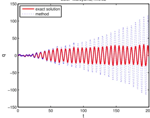
The numerical tests examine the behavior of the numerical methods from three aspects: first, closeness between the os-cillation curves produced by the numerical(��)and the true solution (�(��)), to which Fig. 1, 2, and 3 are contributed; second, ability of preserving the linear growth property (28), as shown by Fig. 4, 5, and 6; and third, the empirical mean-square order of the methods illustrated by Fig. 7 and 8.
Both Fig. 1 and 2, produced by the methods (8) and (9) respectively, exhibit good coincidence between the numerical (blue dotted) and the true solution (red solid) curves, while obviously larger and larger deviation of the numerical curve created by the Euler-Maruyama method (30) from the true solution is observed in Fig. 3, which indicates the effective-ness of the symplectic methods (8) and (9), as well as the invalidity of the non-symplectic Euler-Maruyama method in solving the stochastic oscillator.
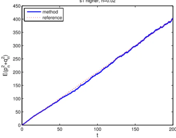
Fig. 4, 5, and 6 show the evolution of the numerical second moment E(�2
� +�
2
�) (blue solid) by the methods (8), (9)
and (30), respectively, compared with the reference line (red dotted) indicating the theoretical path of the linear growth, from which it can be seen that the method (9) preserves the linear growth property (28) more accurately than (8), though both of them behave fairly well in this aspect. The Euler-Maruyama method, however, fails to reproduce the linear growth of the second moment. The expectation E in these tests is approximated by taking average over 500 sample solutions.
0 50 100 150 200
−20 −15 −10 −5 0 5 10 15 20
t
q
s1 lower, h=0.02
exact solution method
Fig. 1. A Sample Trajectory arising from the Numerical Method (8) (blue dotted) and the True Solution (10) (red solid)
0 50 100 150 200
−15 −10 −5 0 5 10 15 20
t
q
s1 higher,h=0.02
exact solution method
Fig. 2. A Sample Trajectory arising from the Numerical Method (9) (blue dotted) and the True Solution (10) (red solid)
0 50 100 150 200
−150 −100 −50 0 50 100 150
t
q
Euler−Maruyama, h=0.02
exact solution method
Fig. 3. A Sample Trajectory arising from the Euler-Maruyama Method (30) (blue dotted) and the True Solution (10) (red solid)
The data for the tests are: (�0, �0) = (0,0), �=� = 1,
�∈[0,200], and the time step-size ℎ= 0.02.
The log-log plot between the step-sizes ℎ and the corresponding mean-square error at � = 200, i.e.
[
E[(��−�(200))2+ (�� −�(200))2]]12
0 50 100 150 200 0
50 100 150 200 250 300 350 400
t
E(p
n
2+q
n
2)
s1 lower, h=0.02
method reference
Fig. 4. Evolution of the Sample Average (over 500 samples) of�2 �+��2
by the Numerical Method (8) (blue solid) and the Exact Second Moment (red dotted)
0 50 100 150 200
0 50 100 150 200 250 300 350 400 450
t
E(p
n
2+q
n
2)
s1 higher, h=0.02
method reference
Fig. 5. Evolution of the Sample Average (over 500 samples) of�2 �+��2
by the Numerical Method (9) (blue solid) and the Exact Second Moment (red dotted)
0 50 100 150 200
0 1000 2000 3000 4000 5000 6000
t
E(p
n
2+q
n
2)
Euler−Maruyama, h=0.02
method reference
Fig. 6. Evolution of the Sample Average (over 500 samples) of�2 �+��2
by the Euler-Maruyama Method (30) (blue solid) and the Exact Second Moment (red dotted)
the numerical plot and the corresponding reference lines that, the mean-square order of (8) is 1, and that of (9) is 2, which coincides with the theoretical results in Proposition 1.
IV. CONCLUSION
Symplectic methods are very important in the simulation of stochastic Hamiltonian systems, especially in long time simulation problems. The paper applies the stochastic gen-erating function approach, which is a systematic way of
−5 −4.5 −4 −3.5 −3 −2.5 −2 −1.5
−5 −4 −3 −2 −1 0 1 2
log(h)
log(ms−error)
s1 order 1
method reference
Fig. 7. Logarithm of the Mean-Square Error at Time �= 200by the Numerical Method (8), versus the Logarithm of the time step-sizeℎ, for h=0.01, 0.02, 0.05, 0.1, 0.2 (blue solid), and the Reference Line of Slope 1 (red dotted)
−5 −4.5 −4 −3.5 −3 −2.5 −2 −1.5
−10 −8 −6 −4 −2 0 2 4
log(ms−error)
s1 order 2
log(h) method
reference
Fig. 8. Logarithm of the Mean-Square Error at Time �= 200by the Numerical Method (9), versus the Logarithm of the time step-sizeℎ, for h=0.01, 0.02, 0.05, 0.1, 0.2 (blue solid), and the Reference Line of Slope 2 (red dotted)
constructing symplectic scheme for stochastic Hamiltonian systems, to a concrete stochastic Hamiltonian system, the linear stochastic oscillator (1), to build symplectic schemes for it, which might serve as a demonstration of the applica-tion of the stochastic generating funcapplica-tion approach. Although only two schemes are given here, many others, in fact, can be produced, by different truncations of the same generating function series, or different choices of generating functions, such as�,�2
or�3
([12]). Construction and implementation of symplectic schemes with even higher orders, however, are still subject to further investigation.
REFERENCES
[1] K. Feng, “On Difference Schemes and Symplectic Geometry”, Pro-ceedings of the 5-th Intern. Symposium on Differential Geometry & Differential Equations, August 1984, Beijing, pp. 42-58, 1985. [2] K. Feng, H.M. Wu, M.-Z. Qin, D.L. Wang, “Construction of
Canon-ical Difference Schemes For Hamiltonian Formalism via Generating Functions”,J Comp Math.7 (1), pp. 71-96, 1989.
[3] E. Hairer, C. Lubich, G. Wanner,Geometric Numerical Integration, Springer-Verlag Berlin Heidelberg, 2002.
[4] D.J. Higham, “An Algorithmic Introduction to Numerical Simulation of Stochastic Differential Equations”,SIAM Rev.43, No. 3, pp. 525-546, 2001.
[6] P.E. Kl¨oden, E. Platen,Numerical Solution of Stochastic Differential Equations, Springer-Verlag Berlin Heidelberg, 1992.
[7] G.N. Milstein,Numerical Integration of Stochastic Differential Equa-tions, Kluwer Academic Publishers, 1995.
[8] G.N. Milstein, YU.M. Repin, M.V. Tretyakov, “Symplectic Integration of Hamiltonian Systems with Additive Noise”,SIAM J. Numer. Anal., Vol. 39, No. 6, pp. 2066-2088, 2002.
[9] G.N. Milstein, YU.M. Repin, M.V. Tretyakov, “Numerical Methods for Stochastic Systems Preserving Symplectic Structure”,SIAM J. Numer. Anal., Vol. 40, No. 4, pp. 1583-1604, 2002.
[10] R.D. Ruth, “A Canonical Integration Technique”,IEEE Trans. Nuclear Science, NS-30, pp. 2669-2671, 1983.
[11] R. de Vogelaere, “Methods of Integration which Preserve the Contact Transformation Property of the Hamiltonian Equations”,Report No. 4, Dept. Math., Univ. of Notre Dame, Notre Dame, Ind., 1956. [12] L. Wang, Variational Integrators and Generating Functions for
Stochastic Hamiltonian Systems, Doctoral Thesis of the University of Karlsruhe, Germany, Universit¨atsverlag Karlsruhe, 2007.