New Trends in Mathematical Sciences
http://www.ntmsci.comOn the Fibonacci and Lucas curves
Mahmut Akyigit, Tulay Erisir and Murat Tosun
Department of Mathematics, Faculty of Arts and Sciences Sakarya University, 54187 Sakarya-Turkey Received: 3 March 2015, Revised: 9 March 2015, Accepted: 19 March 2015
Published online: 16 June 2015
Abstract: In this study, we have constituted the Frenet vector fields of Fibonacci and Lucas curves which are created with the help of Fibonacci and Lucas sequences hold a very important place in nature defined by Horadam and Shannon, [1]. Based on these vector fields, we have investigated notions of evolute, pedal and parallel curves and obtained the graphics of these curves.
Keywords: Fibonacci and Lucas curves, evolute curve, parallel curve, pedal curve.
1 Introduction
One of the most fundamental structure of differential geometry is the theory of curves. An increasing interest of this theory makes a development of special curves to be investigated. A way for classification and characterization of curves is the relationship between the Frenet vectors of the curves. By means of this notions, characterizations of special curves have been revealed, ([3], [5], [8], [9]). Some of these are involute-evolute, parallel and pedal curves etc. C. Boyer discovered involutes while trying to build a more accurate clock, [6]. The involute of a plane curve is constructed from the unit tangent at each point ofF(s), multiplied by the difference between the arc length to a constant and the arc length toF(s). The evolute and involute of a plane curve are inverse operations similar to Differentiation and Integration. Also, in the 17th-century, the firstly pedal curve was found by G. Roberval, [7]. Only in 19th century, more than 500 studies have been conducted on the pedal curves, [10, 11, 13]. Given two curves, one is a parallel curve (also known as an offset curve) of the other if the points on the first curve are equidistant to the corresponding points in the direction of the second curve’s normal. Alternatively, a parallel of a curve can be defined as the envelope of congruent circles whose centers lie on the curve. A parallel of a curve is the envelope of a family of congruent circles centered on the curve. It generalizes the concept of parallel lines. It can be also defined as a curve whose points are at a fixed normal distance of a given curve. More information on the pedal and parallel curves can be found in [14].
The Fibonacci numbers was introduced by Leonardo of Pisa in his book Liber Abaci, [12]. These numbers was used as a model for investigate the growth of rabbit populations. The Fibonacci numbers are closely related to Lucas numbers in that they are a complementary pair of Lucas sequences. They are intimately connected with the golden ratio.
The Fibonacci and Lucas sequence are defined as
and
L0=2, L1=1, Ln=Ln−1+Ln−2
forn≥2, respectively. Here,FnisnthFibonacci number andLnisnthLucas number, ([1], [2], [4], [15], [16]).
2 Preliminaries
To meet the requirements in the next sections, here, the basic elements of the theory of curves in the spaceR2are briefly presented. We restrict our study to local theory of plane curves.
Letr:I→R2be a planar curve, smooth and regular. Firstly, we give without details the two representations of a plane curve.
a) The parametric representation of the plane curve isx=x(s),y=y(s),x′(s)2+y′(s)2>0, ∀s∈I;
b) The implicit representation isF(x,y) =0,F:D→R, D⊆R2,FhasFx′2+Fy′2>0, ∀(x,y)∈D, ([13], [16]).
In this study, we have dealt with the plane curves which defined as parametrical. In parametric form, the equation of the curvature is
k(s) =x′(s)y′′(s)−x′′(s)y′(s) (
(x′)2(s) + (y′)2(s))
3 2 .
If the curve is parametrized by arc-length, the curvature isk(s) =x′(s)y′′(s)−x′′(s)y′(s).
Letr:I→R2be a plane curve. The conditionr′(s)̸=0 is equivalent to the existence of the distinguished Frenet frame. We shall always choose this frame as the moving 2-frame on the curver. So, let {T,N} be Frenet vector field of the planar curverandkbe curvature of this curve. Also, Frenet formulas of the planar curverare as follows
T′ =vkN
N′=−vkT (1)
where∥r′∥=v, ([15], [16]).
Let consider a plane curverand the family of normal to the curve. The envelope of this family is called the evolute of the curver. If the curve is given in parametric form:x=x(s),y=y(s),then the equation of the normal at an arbitrary point r(s)that
y−y(s) =−yx′′((ss))(x−x(s)).
Using the method described in previous paragraph, we can determine the parametric equations of the evolute that
X=x(s)− y ′(s)(
x′2(s) +y′2(s))
x′(s)y′′(s)−x′′(s)y′(s),
Y =y(s) + x ′(s)(
x′2(s) +y′2(s))
x′(s)y′′(s)−x′′(s)y′(s).
that
Pdr(s) =r(s) +
r′(s).(A−r(s)) ∥r′(s)∥2 r
′(s) (2)
whereAis a constant point. If the curvePdris the Pedal curve of the curver, then the curveris negative Pedal curve of the curvePdr, [9].
The parametric equations of the Fibonacci and Lucas curves are given by Horadam and Shannon, [1]. In this study, after we have obtained the Frenet vector fields of the Fibonacci and Lucas taking advantage of [1] we have researched notions of Evolute, Pedal and Parallel curves for this curves.
3 The Fibonacci Curves
LetI⊆Rbe a open interval ofR. So, theFibonacci curveis that
r:I → R2
θ → r(θ) = (x(θ),y(θ)).
If we considerα=1+√5
2 , it is obvious that
x(θ) =α
θ
−α−θ
cos(θ π) √
5 , (3)
y(θ) =−α−
θ
sin(θ π) √
5 (4)
and the graph of the Fibonacci curve is that
Firstly, if we take the derivative of the equations (3.1) and (3.2), with respect toθ, we obtain that
dx dθ =
(
1+√5 2
)−θ[(
1+√5 2
)2θ
log(1+2√5)+log(1+2√5)cos(θ π) +πsin(θ π) ]
√
5 (5)
and
dy dθ =
(
1+√5 2
)−θ[
−πcos(θ π) +log(1+√5
2
)
sin(θ π)] √
Consideringα=1+√5
2 and log( 1+√5
2 ) =s in the equations (3.3) and (3.4), we can find
dx dθ =x
′(θ) =α−
θ[
α2θs+scos(θ π) +πsin(θ π)] √
5 , (7)
dy dθ =y
′(θ) =α−
θ
[−πcos(θ π) +ssin(θ π)] √
5 . (8)
Again taking the derivative of the equations (3.5) and (3.6) with respect toθ, we have
d2x
dθ2=x′′(θ) =
α−θ[(π2−s2)
cos(θ π) +α2θs2−2πssin(θ π)] √
5 , (9)
d2y
dθ2=y′′(θ) =
α−θ[2πscos(θ π) +(π2−s2)sin(θ π)] √
5 . (10)
Now, we will construct the orthonormal frame of the Fibonacci curve at its any points. Consideringv1={x′(θ),y′(θ)} andv2={x′′(θ),y′′(θ)}, we find the orthonormal set benefit from the linear set{v1,v2}. So, we can writev1=u1=
{x′(θ),y′(θ)}andu2=v2−⟨⟨uu1,v2⟩
1,u2⟩u1. If we make necessary arrangement in the latter equation, we get u2={G1,G2}.
where,
G1=
α−θ
(πcos(π θ)−ssin(π θ))(π
(π2+s2) +α2θ
s[3πscos(π θ) + (π2−2s2)sin(π θ)]) √
5{π2+ (1+α4θ)s2+2α2θs[cos(π θ)s+πsin(π θ)]
} .
G2=
α−θ
(Zk1+Zk2) 2√5{π2+s2(1+α4θ) +
2sα2θ[scos(π θ) +πsin(π θ)]
},
including,
Zk1=2π(π2+s2)[scos(π θ) +πsin(π θ)] +2s2α4θ[3πscos(π θ) +(π2−2s2)sin(π θ)],
and
Zk2=−sα2θ[−3π(π2+s2)+π(π2−5s2)cos(2π θ) +2s(−2π2+s2)sin(2π θ)].
ConsideringT= u1
∥u1∥and N= u2
∥u2∥, we can find the orthonormal basis{
T,N}as follows
T=
α−θ(
sα2θ+scos(π θ) +πsin(π θ)) √
2s2cos(π θ) +α−2θ( π2+s2(
1+α4θ)
+lsα)
, α−
θ
(−πcos(π θ) +ssin(π θ))
√
2s2cos(π θ) +α−2θ( π2+s2(
1+α4θ)
+lsα)
(11)
where
lsα=2πsα2θsin(π θ),
N=
πcos(π θ)−ssin(π θ)
√ π2+s2(
1+α4θ)
+2sα2θ(
scos(π θ) +πsin(π θ))
, sα
2θ
+scos(π θ) +πsin(π θ)
√ π2+s2(
1+α4θ)
+2sα2θ(
scos(π θ) +πsin(π θ))
Now, letr:I→R2be the Fibonacci curve and{T,N},kbe Frenet vector fields and curvature of this curve, respectively. So, the relationship between the curvature of the Frenet vector fields is that
T′ =vkN
N′=−vkT (13)
where∥r′∥=v. The formulak= x′y′′−x′y′′ [(x′)2+(y′)2]32
is valid for planar curves. Thus, the curvature function of the Fibonacci
curve is that
k(θ) = √
5[π(π2+s2)α−2θ+3πs2cos(π θ) +s(π2−2s2)sin(π θ)] [α−2θ
{π2+s2(1+α4θ) +
2sα2θ(scos(π θ) +πsin(π θ))
}]3/2. (14)
Also, the parametric equation of evolute of the Fibonacci curver(θ) = (x(θ),y(θ))is that
p(θ) = (X(θ),Y(θ))
where
X(θ) =α −θ{
−2s( π2+s2)
sin(π θ) +2sα4θ
lsπ+π α2θ[2π2−s2+s2cos(2π θ) +πssin(2π θ)]} 2√5{
π( π2+s2)
+sα2θ[
3πscos(π θ) +(
π2−2s2)
sin(π θ)]} ,
lsπ=
[
4πscos(π θ) +(π2−3s2 )
sin(π θ)],
Y(θ) =−
{ sα−θ{
−2Sπ αcos(π θ) +α2θ[−3π2−2s2(3+α4θ)+π2cos(2π θ)−2πs(3α2θ+cos(π θ))sin(π θ)]}} 2√5{π(
π2+s2)
+sα2θ[
3πscos(π θ) +(
π2−2s2)
sin(π θ)]} ,
Sπ α=
[
π2+s2(1+3α4θ)].
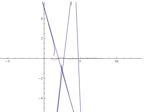
And the relationship between the Fibonacci curve and its evolute is given in Figure 1.
Also, the pedal curve of the Fibonacci curver(θ) = (x(θ),y(θ))given in the equation (2.2) is as follows. In the Figure 2, the Pedal curvesPdr(θ)of the Fibonacci curver(θ)at the points (3,2), (4,2) and (8,2) are plotted.
Figure 2.The Pedal Curves of the Fibonacci Curve.
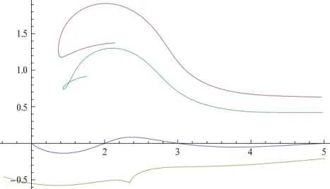
Likewise, the Parallel curvesPlr(θ)of the Fibonacci curver(θ) = (x(θ),y(θ))given in the equation (2.3) is as follows. In the Figure 3, the distances between the Parallel curves and the Fibonacci curve are -0.5, 1 and 1,5, respectively.
Figure 3.The Parallel Curves of the Fibonacci Curve.
4 The Lucas Curves
LetI⊆Rbe open interval ofR. So, theLucas curveis that
r:I → R2
θ → r(θ) = (x(θ),y(θ)).
If we considerα=1+√5
2 , it is obvious that
x(θ) =αθ+α−θcos(θ π), (15)
And the graph of the Lucas curve is that
Firstly, if we take the derivative of the equations (4.1) and (4.2) with respect toθ, we can find that
dx dθ =
(
1+√5 2
)−θ (
1+√5 2
)2θ
log
(
1+√5 2
)
−log
(
1+√5 2
)
cos(π θ)−πsin(π θ)
(17)
dy dθ =
(
1+√5 2
)−θ[
πcos(π θ)−log (
1+√5 2
)
sin(π θ) ]
. (18)
Consideringα=1+√5
2 and log( 1+√5
2 ) =s in the equations (4.3) and (4.4) we have
dx dθ =x
′(θ) =α−θ[sα2θ−scos(π θ)−πsin(π θ)], (19)
dy dθ =y
′(θ) =α−θ[πcos(π θ)−ssin(π θ)]. (20)
Again calculating the derivative of the equations (4.5) and (4.6) with respect toθ, we have
d2x
dθ2=x′′(θ) =α−
θ[(
−π2+s2)
cos(π θ) +s(sα2θ+2πsin(π θ))], (21)
d2y
dθ2=y′′(θ) =α−
θ[
−2πscos(π θ) + (−π2+s2)sin(π θ)]. (22)
Now, we will construct the Frenet vector fields of the Lucas curve.
Letv1={x′(θ),y′(θ)}andv2={x′′(θ),y′′(θ)}be linear independent vectors. We obtain the orthogonal set{u1,u2} from the linear independent set{v1,v2}using the Gram-Schmidt method. So, we can writev1=u1={x′(θ),y′(θ)}and u2=v2−⟨⟨u1u1,,u2v2⟩⟩u1. If we make necessary arrangement in the latter equation, we get
u2=
[
u21,
α−θ(u22+−sα2θ
[
−3π(π2+s2)+π(π2−5s2)cos(2π θ) +2s(−2π2+s2)sin(2π θ)]) 2[π2+s2(1+α4θ)
−2sα2θ(scos(π θ) +πsin(π θ))]
}
,
where
u21=−
α−θ[πcos(π θ)−ssin(π θ)][π(π2+s2)
+sα2θ[
−3πscos(π θ)−(π2−2s2)
sin(π θ)]] π2+s2(1+α4θ)−2sα2θ(scos(π θ) +πsin(π θ)) ,
u22=−2π(π2+s2)(scos(π θ) +πsin(π θ))−2s2α4θ(3πscos(π θ) +(π2−2s2)sin(π θ)).
ConsideringT= u1
∥u1∥andN=
u2
∥u2∥, we can find the orthonormal basis{T,N}as follows
T=
α−θ( sα2θ
−scos(π θ)−πsin(π θ)) √
α−2θ( π2+s2(
1+α4θ))
−2s(scos(π θ) +πsin(π θ))
, α−
θ
(πcos(π θ)−ssin(π θ)) √
α−2θ( π2+s2(
1+α4θ))
−2s(scos(π θ) +πsin(π θ))
(23) and N=
−πcos(π θ) +ssin(π θ) √
π2+s2+s2α4θ
−2s2α2θ
cos(π θ)−2πsα2θ
sin(π θ),
st2θ−scos(π θ)−πsin(π θ) √
π2+s2(
1+α4θ)
−2sα2θ(
scos(π θ) +πsin(π θ))
. (24)
If we make necessary arrangements, we can easily find the curvature function of the Lucas curve that
k(θ) =π (π2
+s2)α−2θ
−3πs2cos(π θ) +s(
−π2+2s2)
sin(π θ)
[α−2θ(π2+s2(1+α4θ))
−2s(scos(π θ) +πsin(π θ))]3/2 (25)
So, the relationship between the curvature of the Frenet vector fields is that
T′ =vkN
N′=−vkT. (26)
where ∥l′∥ = v. Also, the parametric equation of the evolute of the Lucas curve l(θ) = (x(θ),y(θ)) is that
c(θ) = (X(θ),Y(θ))where
X(θ) =−2s
( π2+s2)
sin(π θ) +2sα4θ[
4πscos(π θ) +(
π2−3s2)
sin(π θ)]
−π α2θ[
2π2−s2+s2cos(2π θ) +πssin(2π θ)] −2π(
π2+s2) αθ+
2sα3θ[
3πscos(π θ) +(
π2−2s2)
sin(π θ)] ,
Y(θ) =s
[ −2[
π2+s2(
1+3α4θ)]
cos(π θ) +α2θ{
3π2+2s2(
3+α4θ)
−π2cos(2π θ) +2πs[
−3α2θ+cos(π θ)]
sin(π θ)}]
2π( π2+s2)
αθ
−2sα3θ[
3πscos(π θ) +(
π2−2s2)
sin(π θ)] .
Besides, the relation between the Lucas curve and its evolute is given in Figure 4 that
Also, the Pedal curvePdl(θ)of the Lucas curve l(θ) = (x(θ),y(θ))given in the equation (2.2) is as follows. In the Figure 5, the Pedal curvesPdl(θ)of the Lucas curve at the points(3,2)and(10,2)are plotted.
Figure 5.The Pedal Curves of the Lucas Curve.
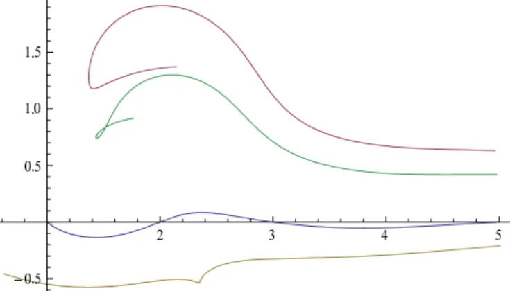
Similarly, the Parallel curvesPll(θ)of the Lucas curvel(θ) = (x(θ),y(θ))given in the equation (2.3) is as follows. In the Figure 6, the distances between the Parallel curves and the Lucas curve are -0.5, 1 and 1,5, respectively.
Figure 6.The Parallel Curves of the Lucas Curve.
References
[1] A. F. Horadam and A. G. Shannon,Fibonacci and Lucas Curves, Fibonacci Quaterly,16no. 1 (1988), 3–13. [2] A. F. Horadam,A Generalized Fibonacci Sequence, American Math. Monthly,68, (1961), 455-459. [3] A. Presley,Elementary Differential Geometry, Springer, (2010).
[4] A. S. Posamentier and I. Lehmann,The (Fabulous) Fibonacci Numbers, Prometheus Books, (2007). [5] C. Bar,Elementary Differential Geometry, Cambridge University Press, (2010).
[6] C. Boyer,A history of Mathematics, New York, Wiley, (1968).
[7] G. Roberval,Divers ouvrages de M. de Roberval dont Observations sur la composition des mouvemens, et sur le moyen de trouver les touchantes des lignes courbes, Paris, (1693).
[9] J. D. Lawrence,A Catalog of Special Plane Curves, New York, Dover, (1972).
[10] J. N. Haton Goupilli,De la courbe qui est elle-meme sa propre podaire, Journal de Mathematiques pures et appliquees S. 2 T,11 no. 1 (1866), 329–336.
[11] J. Steiner,Von dem Kr¨ummungs-Schwerpuncte ebener Curven, Journal f¨ur die reine und angewandte Mathematik,21, (1840), 101–133.
[12] L. E. Sigler,Fibonacci’s Liber Abaci” A Translation into Modern English of Leonardo Pisano’s Book of Calculation, Springer, (2003).
[13] P. Blaga,Lectures on the Differential Geometry of Curves and Surfaces, (2005). [14] R. C. Yates,A Handbook on curves and their properties, Michigan, U.S.A., (1947).