Measurements of nitrogen oxides and ozone fluxes by eddy covariance at a meadow: evidence for an internal leaf resistance to NO<sub>2</sub>

(1)

BGD

10, 4461–4514, 2013

Measurements of nitrogen oxides and

ozone fluxes

P. Stella et al.

Title Page

Abstract Introduction

Conclusions References

Tables Figures

◭ ◮

Back Close

Full Screen / Esc

Printer-friendly Version Interactive Discussion

Discussion

P

a

per

|

Dis

cussion

P

a

per

|

Discussion

P

a

per

|

Discussio

n

P

a

per

|

Biogeosciences Discuss., 10, 4461–4514, 2013 www.biogeosciences-discuss.net/10/4461/2013/ doi:10.5194/bgd-10-4461-2013

Open Access

Biogeosciences

Discussions

Geoscientiic Geoscientiic

This discussion paper is/has been under review for the journal Biogeosciences (BG). Please refer to the corresponding final paper in BG if available.

Measurements of nitrogen oxides and

ozone fluxes by eddy covariance at

a meadow: evidence for an internal leaf

resistance to NO

2

P. Stella1, M. Kortner1,*, C. Ammann2, T. Foken3,4, F. X. Meixner1, and I. Trebs1

1

Max Planck Institute for Chemistry, Biogeochemistry Department, 55020 Mainz, Germany

2

Agroscope ART, Air Pollution and Climate Group, 8046 Z ¨urich, Switzerland

3

University of Bayreuth, Department of Micrometeorology, 95440 Bayreuth, Germany

4

Member of Bayreuth Center of Ecology and Environmental Research (BayCEER), Germany

*

now at: M ¨uller-BBM GmbH, Branch Office Frankfurt, 63589 Linsengericht, Germany

Received: 30 January 2013 – Accepted: 17 February 2013 – Published: 7 March 2013 Correspondence to: P. Stella (patrick.stella@mpic.de)

(2)

BGD

10, 4461–4514, 2013

ozone fluxes

P. Stella et al.

Title Page

Tables Figures

◭ ◮

Back Close

Full Screen / Esc

Discussion

P

a

per

|

Dis

cussion

P

a

per

|

Discussion

P

a

per

|

Discussio

n

P

a

per

|

Abstract

Nitrogen dioxide (NO2) plays an important role in atmospheric pollution, in

particu-lar for tropospheric ozone production. However, the removal processes involved in NO₂ deposition to terrestrial ecosystems are still subject of ongoing discussion. This study reports NO2 flux measurements made over a meadow using the eddy

covari-5

ance method. The measured NO2deposition fluxes during daytime were about a factor

of two lower than a priori calculated fluxes using the Surfatm model without taking into account an internal (also called mesophyllic or sub-stomatal) resistance. Neither an underestimation of the measured NO2 deposition flux due to chemical divergence

or direct NO₂emission, nor an underestimation of the resistances used to model the 10

NO₂ deposition explained the large difference between measured and modelled NO₂ fluxes. Thus, only the existence of the internal resistance could account for this large discrepancy between model and measurements. The median internal resistance was estimated to 300 s m−1 during daytime, but exhibited a large variability (100 s m−1 to 800 s m−1). In comparison, the stomatal resistance was only around 100 s m−1 during 15

daytime. Hence, the internal resistance accounted for 50 % to 90 % of the total leaf resistance to NO₂. This study presents the first clear evidence and quantification of the internal resistance using the eddy covariance method, i.e. plant functioning was not affected by changes of microclimatological (turbulent) conditions that typically occur when using enclosure methods.

20

1 Introduction

Nitrogen oxides (NOx, the sum of nitric oxide, NO, and nitrogen dioxide, NO2) play an

important role in the photochemistry of the atmosphere. By controlling the levels of key radical species such as the hydroxyl radical (OH), NOx are key compounds that

influence the oxidative capacity of the atmosphere. In addition, NOxare closely linked

25

(3)

photo-BGD

10, 4461–4514, 2013

ozone fluxes

P. Stella et al.

Title Page

Tables Figures

◭ ◮

Back Close

Full Screen / Esc

Discussion

P

a

per

|

Dis

cussion

P

a

per

|

Discussion

P

a

per

|

Discussio

n

P

a

per

|

dissociated to NO and ground-state atomic oxygen (O(3P)) that reacts with O2to form

O3(Crutzen, 1970, 1979). O3is a well known greenhouse gas responsible for positive

radiative forcing, i.e. contributing to global warming, representing 25 % of the net ra-diative forcing attributed to human activities since the beginning of the industrial era. Moreover, due to its oxidative capacities, O3is also a harmful pollutant responsible for

5

damages on materials (Almeida et al., 2000; Boyce et al., 2001), human health (Levy et al., 2005; Hazucha and Lefohn, 2007) and plants (Paoletti, 2005; Ainsworth, 2008). In natural environments, O3may lead to biodiversity losses, while in agro-ecosystems,

it induces crop yield losses (Hillstrom and Lindroth, 2008; Avnery et al., 2011a,b; Payne et al., 2011).

10

NOx is also responsible for the production of nitric acid and organic nitrates, both

acid rain and aerosol precursors (Crutzen, 1983). In addition, it influences the forma-tion of nitrous acid (HONO), which is an important precursor for OH radicals in the atmosphere.

The important impacts of NO, NO₂and O₃on both atmospheric chemistry and envi-15

ronmental pollution require to establish the atmospheric budgets of these gases. There-fore, it is necessary (i) to identify the different sources and sinks of NO, NO2 and O3,

and (ii) to understand the processes governing the exchange of these compounds be-tween the atmosphere and the biosphere. To achieve this goal, several studies were carried out in the last decades over various ecosystems to identify the underlying pro-20

cesses controlling the biosphere-atmosphere exchanges of NO (e.g. Meixner, 1994; Meixner et al., 1997; Ludwig et al., 2001; Laville et al., 2009; Bargsten et al., 2010), NO2 (e.g. Meixner, 1994; Eugster and Hesterberg, 1996; Hereid and Monson, 2001;

Chaparro-Suarez et al., 2011; Breuninger et al., 2012), and O₃(e.g. Zhang et al., 2002; Rummel et al., 2007; Stella et al., 2011a).

25

(4)

BGD

10, 4461–4514, 2013

ozone fluxes

P. Stella et al.

Title Page

Tables Figures

◭ ◮

Back Close

Full Screen / Esc

Discussion

P

a

per

|

Dis

cussion

P

a

per

|

Discussion

P

a

per

|

Discussio

n

P

a

per

|

different O₃deposition pathways are well identified and the variables controlling each pathway are well understood: the cuticular and soil ozone deposition pathways are governed by canopy structure (canopy height, leaf area index) and relative humidity at the leaf and soil surface (Zhang et al., 2002; Altimir et al., 2006; Lamaud et al., 2009; Stella et al., 2011a), while stomatal ozone flux is controlled by climatic variables 5

responsible for stomata opening such as radiation, temperature and vapour pressure deficit (Emberson et al., 2000; Gerosa et al., 2004).

However, the processes governing the NO2exchange between the atmosphere and

the biosphere still remain unclear. While it is well recognized that NO2 is mainly

de-posited through stomata, with the cuticular and soil fluxes being insignificant depo-10

sition pathways for NO₂ (Rond ´on et al., 1993; Segschneider et al., 1995; Pilegaard et al., 1998; Geßler et al., 2000; Ludwig et al., 2001), the existence of an internal resis-tance (also called mesophyllic or sub-stomatal resisresis-tance in previous studies) limiting NO₂stomatal uptake is still under discussion. Previous studies reported contrasting re-sults: Segschneider et al. (1995) and Geßler et al. (2000, 2002) did not find an internal 15

resistance for sunflower, beech and spruce, whereas the results obtained by Sparks et al. (2001) and Teklemariam and Sparks (2006) for herbaceous plant species and tropical wet forest suggested its existence. In addition, the importance of this internal resistance for the overall NO2 sink is not well established. Current estimates range

from 3 % to 60 % of the total resistance to NO₂ uptake (Johansson, 1987; Gut et al., 20

2002; Chaparro-Suarez et al., 2011). Nevertheless, all the previous studies explored the processes of NO2 exchange using enclosure (chamber) methods under field or

controlled conditions, which may affect the microclimatological conditions around the plant leaves. This issue is of particular concern since the biochemical processes prob-ably responsible for the internal resistance are linked with leaf functioning (Eller and 25

(5)

BGD

10, 4461–4514, 2013

ozone fluxes

P. Stella et al.

Title Page

Tables Figures

◭ ◮

Back Close

Full Screen / Esc

Discussion

P

a

per

|

Dis

cussion

P

a

per

|

Discussion

P

a

per

|

Discussio

n

P

a

per

|

In this study we present results of the SALSA campaign (SALSA: German acronym for “Contribution of nitrous acid (HONO) to the atmospheric OH-budget”, for details see Mayer et al., 2008). Turbulent fluxes of NO, NO2and O3were measured at a meadow

below the Meteorological Observatory Hohenpeissenberg (MOHp) using the eddy co-variance method. These measurements were accompanied by a comprehensive mi-5

crometeorological setup involving vertical profiles of trace gases and temperature as well as by eddy covariance measurements of carbon dioxide (CO₂) and water vapor fluxes. In the present work, (i) the influence of chemical divergence was estimated above and within the canopy, (ii) the existence of an NO2 compensation point mixing

ratio was explored, (iii) the impact of the soil resistance to modeled NO₂deposition was 10

discussed and (iv) the internal resistance for NO₂was quantified in order to understand the processes governing the NO2exchange.

2 Materials and methods

2.1 Site description

The field study was made at a meadow in the complex landscape around Hohen-15

peißenberg (Southern Germany) within the framework of the SALSA campaign (see Mayer et al., 2008; Trebs et al., 2009). The site consists in a managed and fertilized meadow located at the gentle lower (743 m a.s.l.) WSW-slope (3–4◦) of the mountain Hoher Peißenberg (summit 988 m a.s.l.), directly west of the village Hohenpeißenberg in Bavaria, Southern Germany (coordinates: 47◦48′N, 11◦02′E). The surrounding pre-20

alpine landscape is characterized by its glacially shaped, hilly relief and a patchy land use dominated by the alternation of cattle pastures, meadows, mainly conifer-ous forests and rural settlements. The meadow is growing on clay-rich soil that can be classified as gley-colluvium with very small patches of marsh soil. Furthermore, it was characterized by its relatively low plant biodiversity and consisted mainly of perennial 25

(6)

BGD

10, 4461–4514, 2013

ozone fluxes

P. Stella et al.

Title Page

Tables Figures

◭ ◮

Back Close

Full Screen / Esc

Discussion

P

a

per

|

Dis

cussion

P

a

per

|

Discussion

P

a

per

|

Discussio

n

P

a

per

|

officinale), red clover (Trifolium pratenseL.), white clover (Trifolium repensL.), common cow parsnip (Heracleum sphondyliumL.), sour dock (Rumex acetosaL.), daisy (Bellis perennisL.), and cow parsley (Anthriscus sylvestris(L.) Hoffm.).

The experiment was carried out from 29 August to 20 September 2005. The meadow was mown just before the instrument setup. The canopy height (hc) and leaf area index

5

(LAI) increased from 15 cm and 2.9 m2m−2(at the beginning of the campaign) to 25 cm and 4.9 m2m−2at the end of the experiment, respectively. The roughness length (z0=

0.1hc) ranged from 1.5 cm to 2.5 cm and the displacement height (d=0.7hc) varied

between 10.5 cm and 17.5 cm. These values were confirmed by estimates ofz0andd

from flux and profile records for 10 to 15 September. 10

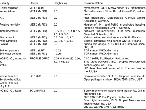
The setup consisted of five measurement stations, (all located in an area of 400 m2, with a distance of 20 to 30 m to each other). The stations recorded meteorological conditions (“MET 1” and “MET 2” from the Bayreuth University (UBT) and the Max Planck Institute for Chemistry (MPIC), respectively), mixing ratio profiles (“PROFILE” from the MPIC) and turbulent fluxes (“EC 1” and “EC 2” from the UBT and the MPIC, 15

respectively) (see Table 1). The detailed measurement setups are described in Table 1 and the following sections.

2.2 Meteorological measurements

The following standard meteorological variables (and vertical profiles) were recorded: global radiation (Gr) and net radiation, relative humidity (RH), air temperature (Ta), wind

20

speed (u) and direction, and rainfall (for details see Table 1). The photolysis rate of NO₂ (jNO₂), soil temperature (Tsoil) and soil water content (SWC) were also measured.

2.3 Trace gas profile measurements

Profile measurements of NO, O3, and NO2 mixing ratios were made in order to

in-vestigate the chemistry of the NO-O₃-NO₂ triad above and within the canopy. The 25

(7)

BGD

10, 4461–4514, 2013

ozone fluxes

P. Stella et al.

Title Page

Tables Figures

◭ ◮

Back Close

Full Screen / Esc

Discussion

P

a

per

|

Dis

cussion

P

a

per

|

Discussion

P

a

per

|

Discussio

n

P

a

per

|

a.g.l.), one at the canopy top (first in 0.20 m, later moved to 0.28 m), and four above the canopy (0.50 m, 1.00 m, 1.65 m and 3.00 m). The NO, O₃, and NO₂analyzers were located in an air conditioned container about 60 m north-east from the air inlets. The profile system was described previously by Mayer et al. (2011). Briefly, air samples from all heights were analyzed by the same analyzer consecutively and the levels were 5

switched automatically by a valve system directly in front of a Teflon®diaphragm pump. The length of the opaque inlet lines made of PFA (perfluoroalkoxy copolymer) ranged from 62 to 65 m (depending on the sampling height). All non-active tubes were con-tinuously flushed by a bypass pump. To avoid condensation of water vapor inside the tubes, they were insulated and heated to a few degrees above ambient temperature. 10

Pressure and temperature in the tubes were monitored continuously. The individual heights were sampled with different frequencies: ambient air from the inlet levels at 0.50 m and 1.65 m were sampled ten times, other levels five times per 60 min (with each interval consisting of three individually recorded 30 s subintervals). Data from the first 30 s interval at each level were discarded to take into account the equilibration time 15

of tubing and analyzers.

NO was measured by red-filtered detection of chemiluminescence – generated by the NO+O₃ reaction – with a CLD 780TR (EcoPhysics, Switzerland). Excess O₃was frequently added in the pre-reaction chamber to account for interference of other trace gases. For the conversion of NO2 to detectable NO, photolysis is the most specific

20

technique (Kley and McFarland, 1980; Ridley et al., 1988). Thus, NO₂ in ambient air was photolytically converted to NO by directing every air sample air through a Blue Light converter (BLC, Droplet Measurement Technologies Inc.). Here, the light source was an UV diode array, which emits radiation within a very narrow spectral band (385– 405 nm), making the NO2to NO conversion more specific and the conversion efficiency

25

(8)

BGD

10, 4461–4514, 2013

ozone fluxes

P. Stella et al.

Title Page

Tables Figures

◭ ◮

Back Close

Full Screen / Esc

Discussion

P

a

per

|

Dis

cussion

P

a

per

|

Discussion

P

a

per

|

Discussio

n

P

a

per

|

(5.0 ppm, Air Liquide). The detection limit of the CLD 780TR was 90 ppt (3σ-definition). The efficiency of the photolytic conversion of NO2to NO was determined by a back

titra-tion procedure involving the reactitra-tion of O3with NO using a gas phase titration system

(Dynamic Gas Calibrator 146 C, Thermo Environmental Instruments Inc., USA). Con-version efficiencies were about 33 %. Ozone mixing ratios of the ambient air samples 5

were measured by an UV absorption instrument (49 C, Thermo Environment, USA).

2.4 Eddy covariance measurements

Eddy covariance has been extensively used during the last decades to estimate turbu-lent fluxes of momentum, heat and (non-reactive) trace gases (Running et al., 1999; Aubinet et al., 2000; Baldocchi et al., 2001; Dolman et al., 2006; Skiba et al., 2009). 10

It is a direct measurement method to determine the exchange of mass and energy between the atmosphere and terrestrial surfaces without application of any empirical constant. The theoretical background for the eddy covariance can be found in existing literature (e.g. Foken, 2008; Foken et al., 2012; Aubinet et al., 2012) and will not be detailed here.

15

The turbulent fluxes of momentum (τ), sensible (H) and latent heat (LE), CO2, NO,

NO₂and O₃were measured by two EC stations (Table 1). One station (MPIC) was ded-icated to the measurement of NO-NO₂-O₃ (as well as momentum and sensible heat,

H) fluxes, while the second (UBT), located∼20 m in the southern direction, measured momentum, H, LE, and CO2 fluxes. The fetch was limited to around 50 m in the NW

20

and NE sector, but extended at least to 150 m in all other directions. Three dimensional wind speed and temperature fluctuations were measured by sonic anemometers (Ta-ble 1) For high-frequency CO2 and water vapor measurements an open-path infrared

gas analyzer (IRGA 7500, LiCor, USA) was used. High frequency (5 Hz) time series of NO and NO2 were determined with a fast-response and highly sensitive closed-path

25

(9)

BGD

10, 4461–4514, 2013

ozone fluxes

P. Stella et al.

Title Page

Tables Figures

◭ ◮

Back Close

Full Screen / Esc

Discussion

P

a

per

|

Dis

cussion

P

a

per

|

Discussion

P

a

per

|

Discussio

n

P

a

per

|

principle of the CLD 790SR-2 is identical to that of the CLD 780TR described above. However, the sensitivity is a factor of 10 higher than that of the CLD 780TR, and due to the presence of two channels the concentrations of NO and NO2can be measured

simultaneously with high time resolution (see Hosaynali Beygi et al., 2011). The ac-curacy of the CLD790SR-2 is about 5 % and the NO detection limit for a one-second 5

integration time is 10 ppt (3σ-definition). The instrument was also located in the air-conditioned container, about 60 m NE from the sonic anemometer. The trace gas inlets were fixed 33 cm below the sound path of the anemometer without horizontal separa-tion at a three-pod mast. Air was sampled through two heated and opaque PFA tubes with a length of 63 m and an inner diameter of 4.4 mm. While the first sample line and 10

CLD channel was used for measuring NO, a BLC converter was placed just behind the sample inlet of the second channel in a ventilated housing mounted at a boom of the measurement mast. Despite the low volume of the BLC (17 mL), conversion effi -cienciesγ for NO₂ to NO of around 41 % were achieved. Consequently this channel detected a partial NOxsignal (denoted here as NO∗x) corresponding to:

15

χ{NO∗_x}=χ{NO}+γ·χ{NO2} (1)

Flow restrictors for both channels of the CLD790SR-2 were mounted into the tubing closely after the corresponding inlets (after the BLC in the second channel) in order to achieve short residence times of the air samples inside the tubing (9±0.4 s and 13±0.4 s for NO and NO2, respectively) and fully turbulent conditions. The EC flux for

20

the two analyzer channels were first calculated independently and the NO₂ flux was then determined as:

FNO₂=

1

γ ·

FNO∗_x−FNO

(2)

Simultaneously, eddy covariance fluxes of O3 were measured with a surface

chemi-luminescence instrument (Table 1) (G ¨usten et al., 1992; G ¨usten and Heinrich, 1996), 25

(10)

BGD

10, 4461–4514, 2013

ozone fluxes

P. Stella et al.

Title Page

Tables Figures

◭ ◮

Back Close

Full Screen / Esc

Discussion

P

a

per

|

Dis

cussion

P

a

per

|

Discussion

P

a

per

|

Discussio

n

P

a

per

|

The 5 Hz signals of both CLD790SR-2 channels, referenced to the frequently cali-brated NO and NO2 measurements at 1.65 m from the trace gas profile system, were

used for the final calculation of NO and NO2fluxes for 30 min time intervals. The O3flux

calibration was done according to Muller et al. (2010). The quality of the derived fluxes was evaluated with the quality assessment schemes of Foken and Wichura (1996) 5

(see also Foken et al., 2004), which validates the development state of turbulence by comparing the measured integral turbulence characteristics. Flux calculations included despiking of scalar time series (Vickers and Mahrt, 1997), planar fit coordinate rota-tion (Wilczak et al., 2001), linear detrending, correcrota-tion of the time lag induced by the 63 m inlet tube, and correction for flux losses due to the attenuation of high frequency 10

contributions according to Spirig et al. (2005) based on ogive analysis (Oncley, 1989; Desjardins et al., 1989). The high frequency losses were typically 12–20 % for NO, 16– 25 % for NO2 and 6–8 % for O3. Since pressure and temperature were held constant

by the instruments and the effect of water vapor fluctuations was negligible, corrections for density fluctuations (WPL-corrections, Webb et al., 1980) were not necessary for 15

NO, NO2and O3.

2.5 Resistance model parameterisations

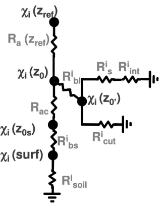
The transfer of heat and trace gases can be assimilated into a resistance network with analogy to the Ohm’s law (Wesely, 1989; Wesely and Hicks, 2000). It includes the tur-bulent resistance above (Ra) and within (Rac) the canopy, the quasi-laminar boundary

20

layer (Rb), the stomatal (Rs) and internal (Rint) resistances, the cuticular resistance

(Rcut) and the soil resistance (Rsoil).

In order to investigate the processes governing the exchanges of NO2 and O3, we

used the Surfatm model developed to simulate exchanges of heat and pollutant be-tween the atmosphere and the vegetation (Personne et al., 2009; Stella et al., 2011b). It 25

(11)

BGD

10, 4461–4514, 2013

ozone fluxes

P. Stella et al.

Title Page

Tables Figures

◭ ◮

Back Close

Full Screen / Esc

Discussion

P

a

per

|

Dis

cussion

P

a

per

|

Discussion

P

a

per

|

Discussio

n

P

a

per

|

trace gas exchange. It comprises one vegetation layer and one soil layer. This model was initially developed to simulate the ammonia exchange and it was validated over grasslands by Personne et al. (2009), and recently adapted to estimate O3 deposition

to several maize crops by Stella et al. (2011b). In the following, we will only focus on the specific resistances to NO₂ and O₃ deposition. However, more details and expla-5

nations concerning the resistive scheme and the resistance parameterizations can be found in Personne et al. (2009) and Stella et al. (2011b).

The resistive scheme for NO₂ and O₃ deposition is shown in Fig. 1. Turbulent re-sistances above and within the canopy are identical for both NO2 and O3, and were

expressed as: 10

Ra(zref)=

1

k2_·_u₍_z ref)

·

ln

_z

ref−d

z0T

−ΨH((zref−d)/L)

·

ln

_z

ref−d

z0M

−ΨM((zref−d)/L)

(3)

Rac=

hc·exp (αu)

α_u·K_M(hc) ·

exp

₋_α

u·z0s

hc

−exp

₋_α

u·(d+z0M)

hc

(4)

where k (=0.4) is the von K ´arm ´an’s constant, zref is the reference height, d is the

15

displacement height, z_0T and z_0M are the canopy roughness length for temperature and momentum respectively,z0s(=0.02 m; Personne et al., 2009) is the ground surface

roughness length below the canopy,hc is the canopy height,u(zref) is the wind speed

at zref, αu (=4.2) is the attenuation coefficient for the decrease of the wind speed

inside the canopy (Raupach et al., 1996),KM(hc) is the eddy diffusivity at the canopy

20

height, andΨM((zref−d)/L) andΨH((zref−d)/L) are dimensionless stability correction

functions for momentum and heat, respectively (Dyer and Hicks, 1970).

The canopy (Rbl) and soil (Rbs) quasi-laminar boundary layer resistances depend

(12)

BGD

10, 4461–4514, 2013

ozone fluxes

P. Stella et al.

Title Page

Tables Figures

◭ ◮

Back Close

Full Screen / Esc

Discussion

P

a

per

|

Dis

cussion

P

a

per

|

Discussion

P

a

per

|

Discussio

n

P

a

per

|

(1985) and Choudhury and Monteith (1988), and Hicks et al. (1987), respectively, as:

R_bli = Di

D_H

2O

· αu

2·a·LAI·

LW

u(hc)

0.5

·

1−exp

−αu

2 −1

(5)

R_bsi = 2

k·u_∗ground ·

_Sc

i

Pr 2/3

(6)

where a is a coefficient equal to 0.01 s m−1/2 (Choudhury and Monteith, 1988), LW 5

(=0.05 m) is the characteristic width of the leaves, D_i and DH₂O are the diffusivities

of the gasi and water vapour respectively (DO₃/DH₂O=0.66 andDNO₂/DH₂O=0.62;

Massman, 1998), Sc_i and Pr are the Schmidt number for the gas i and the Prandtl number ((Sc_O

3/Pr)

2/3

=1.14 for O₃and (Sc_NO 2/Pr)

2/3

=1.19 for NO₂; Erisman et al., 1994), andu_∗groundis the friction velocity near the soil surface calculated following

Lou-10

bet et al. (2006) as:

u_∗ground=

(u∗)2·exp

1.2·LAI·

_z

0s

hc

−1

0.5

(7)

whereu_∗ is the friction velocity above the canopy.

The stomatal resistance was not modelled but used as input. It was inferred from wa-ter vapour flux measurements by inverting the Penman–Monteith equation (Monteith, 15

1981):

R_si

PM=   

 

Di

DH₂O

·

E δ_w

1+_δE w ·

Ra+Rbi

·β_γ·s−1

  

 

−1

(8)

whereE is the water vapour flux (kg m−2s−1), δw the water vapour density saturation

(13)

BGD

10, 4461–4514, 2013

ozone fluxes

P. Stella et al.

Title Page

Tables Figures

◭ ◮

Back Close

Full Screen / Esc

Discussion

P

a

per

|

Dis

cussion

P

a

per

|

Discussion

P

a

per

|

Discussio

n

P

a

per

|

the psychrometric constant (K−1). However,R_s_PM can be defined as the stomatal resis-tance ifE represents plant transpiration only, i.e. the influence of soil evaporation and evaporation of liquid water (rain, dew) that may be present at the canopy surface has to be excluded. Thus, our estimation of stomatal resistance was corrected for water evaporation as proposed by Lamaud et al. (2009): for dry conditions (RH<60 %, for 5

which liquid water at the leaf surface is considered to be completely evaporated)Rs_PM

was plotted against Gross Primary Production (GPP, estimated on a daily basis follow-ing Kowalski et al., 2003, 2004). The corrected stomatal resistance (Rs) for all humidity

conditions is then given by:

R_si = Di

DH₂O

α·GPPλ (9)

10

whereα(=7465) andλ(=−1.6) are coefficients given by the regression betweenR_s

PM and GPP under dry conditions.

The soil and cuticular resistances to O3deposition were expressed following Stella

et al. (2011a,b) as:

RO3

soil=Rsoil_min·exp (ksoil·RHsurf) (10)

15

RO3

cut=Rcut_max if RHz′

0<RH0 (11a)

RO3

cut=Rcut_max·exp(−kcut·(RHz′

0−RH0)) if RHz′0>RH0 (11b)

whereRsoilmin (=21.15 s m

−1

) is the soil resistance without water adsorbed at the soil 20

surface (i.e. at RHsurf=0 %),ksoil(=0.024) is an empirical coefficient of the exponential

function,R_cutmax(=5000/LAI) is the maximal cuticular resistance calculated according to Massman (2004), RH0 (=60 %) is a threshold value of the relative humidity, kcut

(=0.045) is an empirical coefficient of the exponential function taken from Lamaud et al. (2009), and RHsurfand RHz′

0are the relative humidity at the soil and leaf surface, 25

(14)

BGD

10, 4461–4514, 2013

ozone fluxes

P. Stella et al.

Title Page

Tables Figures

◭ ◮

Back Close

Full Screen / Esc

Discussion

P

a

per

|

Dis

cussion

P

a

per

|

Discussion

P

a

per

|

Discussio

n

P

a

per

|

Concerning the NO₂ cuticular resistance, several studies showed that this deposi-tion pathway did not contribute significantly to NO2deposition and could be neglected

(Rond ´on et al., 1993; Segschneider et al., 1995; Gut et al., 2002). Consequently,RNO2

cut

was set to 9999 s m−1. Since an empirical parameterization for the soil resistance to NO2deposition is currently not available, a constant value (R

NO₂

soil =340 s m

−1

) reported 5

by Gut et al. (2002) for a soil in the Amazonian rain forest was used.

Finally, many trace gases entering into plants through stomata can react with com-pounds in the sub-stomatal cavity and the mesophyll. For O3, there is evidence thatRint

is usually zero (Erisman et al., 1994). However, for NO2there is currently no consensus

concerning the existence of an internal resistance, and the uncertainty of the magni-10

tude of its contribution to the overall surface resistance is large. Due to this insufficient knowledge,Rintwas also set to zero for NO2in the “a priori” model parameterization.

The total deposition flux of the scalari (Fi) is the sum of deposition flux to the soil

(F_soili ) and the deposition flux to the vegetation (Fvegi ):

Fi =F_soili +Fvegi (12)

15

In analogy to Ohm’s law and following the resistive scheme of the Surfatm model (Fig. 1), total, vegetation and soil fluxes can be expressed as:

F_i =χi(z0)−χi(zref)

Ra(zref)

(13)

F_vegi = −χi(z0)

R_bli +

1 R_cuti +

1 Ri_s+R_inti

−1 (14)

F_soili = −χi(z0)

Rac+R_bsi +R_soili

(15)

BGD

10, 4461–4514, 2013

ozone fluxes

P. Stella et al.

Title Page

Tables Figures

◭ ◮

Back Close

Full Screen / Esc

Discussion

P

a

per

|

Dis

cussion

P

a

per

|

Discussion

P

a

per

|

Discussio

n

P

a

per

|

The deposition flux to soil can also be expressed as:

F_soili =χi(z0s)−χi(z0)

Rac

(16)

F_soili = −χi(z0s)

R_bsi +R_soili (17)

2.6 Chemical reaction and transport times

5

In contrast to inert gases such as CO₂and H₂O, the fluxes of NO, NO₂ and O₃could be subject to chemical reactions leading to non-constant fluxes with height (vertical flux divergence). According to Remde et al. (1993) and Warneck (2000), the main gas phase reactions for the NO-O₃-NO₂triad are:

NO+O3 k_r

−→NO2+O2 (R1)

10

NO2+O2+hν j_NO2

−→NO+O3 (R2)

wherek_r is the rate constant of R1 (Atkinson et al., 2004) andj_NO

2 is the photolysis frequency for R2.

The chemical reaction time for NO-O3-NO2triad (τchem in s) gives the characteristic

time scale of the set of R1 and R2. It was estimated following the approach of Lenschow 15

(1982):

τchem=2

.h

j_NO2

2+k

2

r ·(O3−NO)2+2·jNO₂·kr(O3+NO+2·NO2)

i0.5

(16)

BGD

10, 4461–4514, 2013

ozone fluxes

P. Stella et al.

Title Page

Tables Figures

◭ ◮

Back Close

Full Screen / Esc

Discussion

P

a

per

|

Dis

cussion

P

a

per

|

Discussion

P

a

per

|

Discussio

n

P

a

per

|

In addition, the characteristic chemical depletion times for NO, O₃ and NO₂were cal-culated according to De Arellano and Duynkerke (1992):

τdeplNO=

1

kr·O3

(19a)

τdeplO₃=

1

k_r·NO (19b)

τdeplNO₂=

1

jNO₂

(19c) 5

The comparison of characteristic chemical reaction times with characteristic turbulent transport times indicates whether or not there is a significant vertical divergence of the turbulent flux of reactive trace gases. The transport time (τtrans in s) in one layer (i.e.

above the canopy, between the measurement height and the canopy top, or within the 10

canopy) can be expressed as the aerodynamic resistance through each layer multiplied by the layer thickness (Garland, 1977):

τtrans=Ra(zref)·(zref−d−z0) above the canopy (20a)

τtrans=Rac·(d+z0−z0s) within the canopy (20b)

15

The ratio between τtrans and τchem is defined as the Damk ¨ohler number (DA)

(Damk ¨ohler, 1940):

DA= τtrans

τchem

(21)

According to Damk ¨ohler (1940), the divergence of a reactive trace gas flux is neg-ligible if DA≪1 (conventionally DA≤0.1), i.e. the turbulent transport is much faster 20

(17)

BGD

10, 4461–4514, 2013

ozone fluxes

P. Stella et al.

Title Page

Tables Figures

◭ ◮

Back Close

Full Screen / Esc

Discussion

P

a

per

|

Dis

cussion

P

a

per

|

Discussion

P

a

per

|

Discussio

n

P

a

per

|

2.7 Estimation of NO-O3-NO2flux divergences above the canopy

The measured NO2-O3-NO fluxes were corrected for chemical reactions occurring

be-tween the canopy top and the measurement height using the method proposed by Duyzer et al. (1995)

Duyzer et al. (1995) demonstrated that the general form of the flux divergence is: 5

(∂F_i/∂z)_z=a_iln(z)+b_i (22)

The factorai is calculated for NO2, NO and O3as:

aNO₂=−aNO=−aO₃=−

ϕ_X

ku∗

h

kr(NO·FO₃+O3·FNO)−jNO₂·FNO₂

i

(23)

whereϕ_X =ϕNO=ϕO₃ =ϕNO₂=ϕH is the stability correction function for heat (Dyer

and Hicks, 1970). As shown by Lenschow and Delany (1987), the flux divergence at 10

higher levels approaches zero. The factor bi was calculated for NO2, NO and O3 as

b_i =−a_iln(zref), assuming that at zref=2 m the flux divergence was zero. For each

compound, the corrected flux (F_i_,corr) is then approximated as:

Fi,corr=Fi+ d

Z

zref _∂F

i

∂z

z

d z=Fi+aizref(1+ln(d /zref)) (24)

3 Results and discussion

15

3.1 Meteorological conditions and mixing ratios

During the experimental period, the median value of the mean diel course of global ra-diation (Gr) reached its maximum of∼700 Wm−

2

(18)

BGD

10, 4461–4514, 2013

ozone fluxes

P. Stella et al.

Title Page

Tables Figures

◭ ◮

Back Close

Full Screen / Esc

Discussion

P

a

per

|

Dis

cussion

P

a

per

|

Discussion

P

a

per

|

Discussio

n

P

a

per

|

humidity (RH) decreased during the morning to reach its minimum of 65 % after noon (Fig. 2b). The meteorological conditions were different during the first half of the ex-periment (29 August to 9 September 2005) and the second half (10 to 20 September 2005). While the former period was sunny and warm and characterized by easterly flows, the latter was dominated by rainy, cold, and overcast conditions governed by 5

westerly winds. This resulted in considerable variability of the meteorological condi-tions during the experiment: maximalGr andTaranged between 200−800 Wm−

2

, and 15−25◦C, respectively, and minimal RH varied between 80–50 % (Fig. 2a, b).

Mean diel courses of NO2, NO and O3mixing ratios measured at 1.65 m a.g.l. (profile

system) are shown in Fig. 2c. Median NO mixing ratios were close to zero during the 10

major part of the experiment and slightly increased during the morning to about 1 ppb. These elevated NO values occurred when the NO2 mixing ratio began to decrease

due to photolysis. In addition, some NO was most likely advected from roads passing the site at a distance of 2 km in NE from the experimental site. Highest mixing ratios of NO2 were on average about 6 ppb during the early morning and 4 ppb during the

15

late afternoon, but increased occasionally up to 8 ppb. During the rest of the day, NO2

mixing ratios were around 2–3 ppb. The diel trend of NO₂was linked with photochem-istry: during sunrise, NO2 photolysis led to the decrease in NO2 mixing ratios, while

during nighttime the absence of photolysis and the stable stratification induced an ac-cumulation of NO₂ in the lower troposphere. O₃mixing ratios exceeded NO and NO₂ 20

mixing ratios and varied from 10 to 20 ppb during nighttime and from 40 to 60 ppb dur-ing daytime. Durdur-ing the morndur-ing, turbulent mixdur-ing in the planetary boundary layer led to entrainment of O₃ from the free troposphere (Stull, 1989). In addition, photochemical O3 production (in the presence of NOx and volatile organic compounds) caused the

increase of O3mixing ratios during the morning, reaching its maximum in the early

af-25

ternoon. The O₃removal by dry deposition processes and the reduced entrainment of O3from the free troposphere as a result of thermally stable stratification and low wind

(19)

BGD

10, 4461–4514, 2013

ozone fluxes

P. Stella et al.

Title Page

Tables Figures

◭ ◮

Back Close

Full Screen / Esc

Discussion

P

a

per

|

Dis

cussion

P

a

per

|

Discussion

P

a

per

|

Discussio

n

P

a

per

|

during the night (c.f., Coyle et al., 2002). Overall, NO₂and O₃mixing ratios were higher from 29 August 2005 to 9 September 2005 than from 10 to 20 September 2005.

3.2 Footprint analysis and measured fluxes

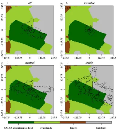
Since the three-pod mast, the laboratory container and some rural settlements were potentially distorting the flow in the north and in the eastern sector of our site, we per-5

formed a footprint analysis according to G ¨ockede et al. (2004, 2006). Owing to the extended fetch in western, southern and south-eastern directions, the major part of the fluxes measured by the EC systems originated from the experimental field, indepen-dently of the stability conditions (Fig. 3). However, the surrounding areas contributed to the total fluxes mainly in the NNW/NE sectors, due to (i) the limited fetch and (ii) the 10

rural settlements disturbing the flow in these directions. In addition, the footprint area increased with atmospheric stability. In order to ensure that only those measured fluxes which originated from the experimental field (an not from the surrounding areas) were used for subsequent analyses, we considered only those 30 min flux data for which at least 95 % of the total footprint area could be attributed to the experimental field. 15

NO2 and O3 fluxes were directed downward, i.e. net deposition fluxes were

ob-served (Fig. 2d). Both NO₂ and O₃deposition fluxes were close to zero during night-time and typically increased during the morning to their maximum. Maximum de-position fluxes of NO2 occurred in the early morning and ranged on average from

about−0.3 nmol m−2s−1to−0.6 nmol m−2s−1. The deposition fluxes of O3were about

20

10 to 20 times higher than NO₂ fluxes ranging on average from −7 nmol m−2s−1 to

−12 nmol m−2s−1 at noon. The calculated deposition velocities for NO2 and O3

exhib-ited a similar diel course and increased during the morning, reaching their maximum and decreasing during afternoon. Despite similar deposition velocities during night-time (∼0.1 cm s−1), the maximal median deposition velocity for NO2 was two times

25

lower than for O3 during daytime (around 0.3 cm s− 1

for NO2 and 0.6 cm s− 1

for O3)

(20)

BGD

10, 4461–4514, 2013

ozone fluxes

P. Stella et al.

Title Page

Tables Figures

◭ ◮

Back Close

Full Screen / Esc

Discussion

P

a

per

|

Dis

cussion

P

a

per

|

Discussion

P

a

per

|

Discussio

n

P

a

per

|

during nighttime and were directed upward during daytime, i.e. indicating net emission, with maxima of 0.05–0.1 nmol m−2s−1during daytime (see Fig. 2d).

3.3 Model vs. measurements: fluxes and mixing ratios

The O3 fluxes estimated using the Surfatm model agreed well with those measured

during the whole experimental period. The linear regression showed that the model 5

underestimated the measured fluxes by only 2 % on average (Fig. 4a). We attempted another step of validation of the Surfatm model by comparing measured and model derived O3mixing ratios at two crucial levels, namely atz0andz0s. For that O3mixing

ratios were estimated (a) at z0 estimated from Eq. (13) using the measured O3 flux,

the measured O3 mixing ratio at zref and modelled Ra, and (b) at z0s from Eq. (16)

10

using the modelled O3 soil flux, the measured O3 mixing ratio at 20 cm (later moved

at 28 cm) and modelledRac values. In Fig. 4b, c these O3 mixing ratios are shown in

comparison (a) to the O3mixing ratio measured at 20–28 cm assuming that 20–28 cm

was representative of z0, and (b) to the measured O3 mixing ratio at 5 cm assuming

that this level was representative ofz0s. At least during daytime, the modelled O3mixing

15

ratios just above the canopy and the soil agree very well with the measurement, which validates the applied values ofRaandRac(necessary to estimate transport times above

and within the canopy; see Sect. 2.6). This result is indeed justified also by the fact, that O3 mixing ratios modelled with ±50 % ofRaand Rac (red dashed lines in Figs. 4b, c)

largely deviate from measured mixing ratios. The good agreement for O3indicates that

20

the resistances used to model O₃fluxes were valid and consequently represent the O₃ exchange processes quite well.

The turbulent resistances (i.e. Ra and Rac) used to model NO2 deposition fluxes

are identical to those used for modelling the O₃ fluxes (only modulated by different molecular diffusivities; see Sect. 2.5). Thus, the good agreement between measured 25

and modelled O3fluxes and mixing ratios would suggest to apply resistancesRa,Rac,

(21)

BGD

10, 4461–4514, 2013

ozone fluxes

P. Stella et al.

Title Page

Tables Figures

◭ ◮

Back Close

Full Screen / Esc

Discussion

P

a

per

|

Dis

cussion

P

a

per

|

Discussion

P

a

per

|

Discussio

n

P

a

per

|

However, a priori modelled NO2 deposition fluxes (withR NO₂

int =0) do not agree well

with the measured NO₂ fluxes during the SALSA campaign (Fig. 5). The relationship between measured and modelled NO₂ fluxes showed a significant scatter (R2=0.45) and a large deviation (slope=1.22) from the 1 : 1 line (Fig. 5a). The NO2 fluxes

dur-ing nighttime were quite well reproduced by the model with an absolute difference 5

varying around zero (Fig. 5b). However, this small absolute difference caused a large relative difference between measured and modelled fluxes, indicating an underesti-mation by the model of around 50 %, which was due to the small NO2 fluxes during

nighttime (Fig. 2d). Nevertheless, during daytime the NO₂ deposition was significantly overestimated. The difference between measured and modelled NO2fluxes increased

10

during the morning, reached its maximum at noon and decreased during the after-noon (Fig. 5b). At after-noon, the modelled NO₂ fluxes were typically two times larger than the measured NO2fluxes, and this overestimation could occasionally reach a factor of

three (Fig. 5b).

It is now required to understand the reasons responsible for this substantial overes-15

timation of the a priori modelled NO2deposition. These reasons could be separated in

two categories: (i) the measured NO2 fluxes were not only caused by turbulent

trans-port of NO₂towards the surface and/or (ii) the resistances to NO₂deposition used in the model were underestimated. On one hand, the EC method measures the flux at a spe-cific height (zref=2 m). For reactive species such as NO2, chemical reactions in the air

20

column within or above the canopy could induce a flux divergence with height, meaning that the flux at the measurement height is different than the flux close to the surface, which is in contrast to inert species such as water vapour or CO2 (e.g. Kramm et al.,

1991, 1996; Galmarini et al., 1997; Walton et al., 1997). If the characteristic turbulent transport times (see Eq. 20) are not significantly shorter than characteristic chemical 25

(22)

BGD

10, 4461–4514, 2013

ozone fluxes

P. Stella et al.

Title Page

Tables Figures

◭ ◮

Back Close

Full Screen / Esc

Discussion

P

a

per

|

Dis

cussion

P

a

per

|

Discussion

P

a

per

|

Discussio

n

P

a

per

|

NO₂ exists, the deposition flux estimated by the model would be larger than the mea-sured net flux. On the other hand, the model could also overestimate NO2deposition,

which implies that the applied resistance parameterisations in the model might be not complete. However, as explained previously, this was not the case forRa,Rac,Rbl,Rbs,

andRssince they were validated owing to the good agreement between measured and

5

modelled O3fluxes. Thus, if we presume that the cuticular deposition is negligible (i.e.

RNO2

cut =9999 s m

−1

) as shown previously (see above), only the remaining resistances

RsoilandRintfor NO2could be underestimated. In the following, each reason that may

explain the overestimation of NO2deposition by the model is explored and discussed.

3.4 Impact of chemical reactions on NO2fluxes 10

Transport and chemical reaction times were estimated above and within the canopy in order to determine to what extent chemical depletion or production in the air column could affect the measured NO2fluxes.

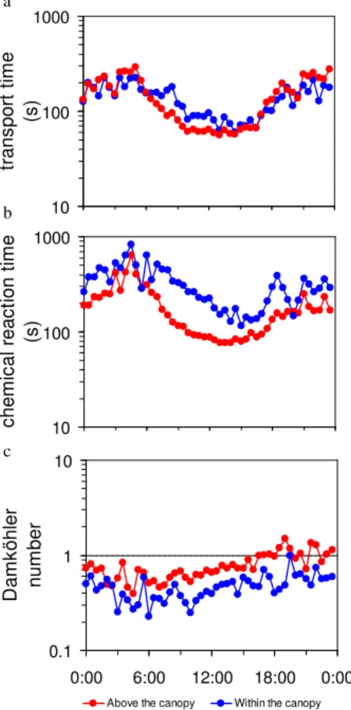
Characteristic transport times (τtrans) for both above and within the canopy followed

a diurnal cycle (Fig. 6a). It was larger during nighttime and decreased during the morn-15

ing to reach its minimum in the early afternoon. It then increased during the after-noon until the sunset. Despite the difference of the layer height (above the canopy:

zref−d=1.60 m and 1.50 m at the beginning and the end of the experiment,

respec-tively; within the canopy: d−z0s=0.10 m and 0.19 m at the beginning and the end

of the experiment, respectively),τtrans was comparable above the canopy and within

20

the canopy. It was about 200 s during nighttime and decreased to about 55 s above the canopy and to 80 s within the canopy at noon. The lower turbulence and stable atmospheric conditions during nighttime induced a slower turbulent transport, while the unstable atmospheric conditions and turbulent mixing enhanced reducedτtrans.

Al-thoughτtrans was comparable above and within the canopy, it must be kept in mind that

25

(23)

BGD

10, 4461–4514, 2013

ozone fluxes

P. Stella et al.

Title Page

Tables Figures

◭ ◮

Back Close

Full Screen / Esc

Discussion

P

a

per

|

Dis

cussion

P

a

per

|

Discussion

P

a

per

|

Discussio

n

P

a

per

|

This implies that the “transfer velocity” was significantly lower within the canopy than above.

Characteristic chemical reaction times were calculated above and within the canopy. Above the canopy,τchem was calculated using Eq. (18), i.e. taking into account both

NO₂ photolysis and NO₂ production by the reaction between O₃ and NO. However, 5

jNO₂ was not measured inside the canopy, hence;τchem could not be calculated using

Eq. (18). Since jNO₂ is closely related to Gr (see Trebs et al., 2009), which typically

sharply decreases in a dense canopy, NO₂ photolysis was assumed to be negligible. In addition, the measured O3 mixing ratio at 0.05 m above ground level was about

10 times larger than the measured NO mixing ratio in the early morning and up to 10

30 times larger during the afternoon and nighttime (data not shown). The reaction between NO and O3is a second order reaction, but can be approximated by a

pseudo-first order reaction because O3was in excess compared to NO. The pseudo-first order

reaction rate constant is defined as kr′=kr·O3 (in s

−1

), and τchem inside the canopy

can be approximated as the chemical depletion time for NO (Eq. 19a). The chemical 15

reaction time followed the same diurnal cycle above and within the canopy: it reached its maximum in the early morning, progressively decreased to reach a minimum in early afternoon, and increased from the early afternoon to the early morning (Fig. 6b). Despite of the comparable diurnal cycle above and within the canopyτchem above the

canopy was usually faster than inside the canopy. The chemical reaction time above the 20

canopy peaked at 300 s and decreased to 80 s, whereas inside the canopy it reached 600 s and decreased to only 150 s (Fig. 6b).

The DA values calculated from Eq. (21) were usually lower than unity, implying that in general turbulent transport was faster than chemical reactions, although DA was occa-sionally close to unity (Fig. 6c). In addition, DA was larger above the canopy than within 25

(24)

BGD

10, 4461–4514, 2013

ozone fluxes

P. Stella et al.

Title Page

Tables Figures

◭ ◮

Back Close

Full Screen / Esc

Discussion

P

a

per

|

Dis

cussion

P

a

per

|

Discussion

P

a

per

|

Discussio

n

P

a

per

|

can be treated as non-reactive only for DA<0.1, and that chemical divergence could be of minor importance for 0.1<DA<1. For example, Stella et al. (2012) demonstrated that chemical reactions induced a flux divergence for O3and NO accounting for 0 % to

25 % of the measured fluxes for 0.1<DA<1.

Consequently, the impact of chemistry above the canopy on measured NO₂ fluxes 5

was evaluated using the method proposed by Duyzer et al. (1995). According to this method, chemistry between NO, NO2 and O3 above the canopy could induce only

a small divergence. The median difference between the measured and the corrected NO2fluxes varied between±0.025 nmol m−

2

s−1, which corresponded to a relative dif-ference of±10 % (Fig. 7a), whereas the difference between measured and modelled 10

NO₂ fluxes was about 20 times larger (absolute difference ≈0.40 nmol m−2s−1, ratio

≈2 during daytime; see Fig. 5b and Sect. 3.3). Hence, chemistry above the canopy did not explain the large overestimation of NO2deposition fluxes by the model. In addition,

similarly to O₃, the NO₂mixing ratio was estimated atz0from Eq. (13) using the

mea-sured NO2flux, the measured NO2mixing ratio atzrefand modelledRa, and compared

15

with NO2 mixing ratio estimated at 20–28 cm (Fig. 7b). Since the resistance analogy

implies the absence of chemical reactions, the good agreement between measured and modelled NO2mixing ratio above the canopy also confirmed the non significance

of chemistry above the canopy, at least during daytime. Nevertheless, during nighttime, discrepancies occurred between measured and modelled NO₂ mixing ratios, meaning 20

that fast chemistry cannot be discarded.

These methods could not be used to estimate the influence of chemical reactions inside the canopy since (i) the method proposed by Duyzer et al. (1995) is only based on mass conservation of the NO-O3-NO2 triad and it does not integrate the different

emission or deposition processes that could occur inside the canopy, and (ii) the com-25

parison of measured and modelled NO₂ mixing ratios inside the canopy (i.e. at 5 cm) requires knowledge of the modelled soil NO2 flux, or at least the vegetation flux (to

deduce the soil flux from the difference between total and vegetation NO2flux), which

(25)

BGD

10, 4461–4514, 2013

ozone fluxes

P. Stella et al.

Title Page

Tables Figures

◭ ◮

Back Close

Full Screen / Esc

Discussion

P

a

per

|

Dis

cussion

P

a

per

|

Discussion

P

a

per

|

Discussio

n

P

a

per

|

results suggest that the impact of NO-O₃-NO₂ chemistry inside the canopy could be negligible. The calculated DA numbers did not indicate that chemistry was dominating the exchange inside the canopy. In addition, the DA number inside the canopy was lower than above the canopy (Fig. 6c), which implies that chemistry inside the canopy was probably even less important than above the canopy.

5

3.5 Compensation point for NO2

In order to investigate the existence of a NO2 emission flux that may partially

com-pensate the NO2deposition flux, thus, causing an overestimation of the modelled NO2

deposition flux, the existence of a canopy compensation point (the NO₂ mixing ratio just above the vegetation elements at which consumption and production processes 10

balance each other) was explored. Figure 8 shows the measured NO2fluxes corrected

for chemical reactions above the canopy versus the measured NO₂mixing ratios. Only data for Gr>400 Wm

−2

were considered, a threshold above which stomatal conduc-tance is supposed to be constant. The linear regression between the NO2flux and the

NO₂mixing ratio did not show an intersection of the regression line with the x-axis (NO₂ 15

mixing ratio) within the error of the regression at the 95 % confidence interval. Hence, these results do not suggest the existence of a canopy compensation point, and thus indicate the non-existence of a NO₂ emission flux at the meadow. In addition, this re-sult also supports the small influence of chemical NO2 production inside the canopy,

as stated previously. 20

The existence of the NO₂ compensation point, as well as its magnitude, is cur-rently subject to debate (Lerdau et al., 2000). Numerous studies carried out over sev-eral ecosystems such as forests, crops and grasslands reported NO2 compensation

points on the leaf or branch level ranging from less than 0.1 ppb to up to 1.5 ppb (Jo-hansson, 1987; Weber and Rennenberg, 1996; Gebler et al., 2000, 2002; Hereid and 25

Monson, 2001; Teklemariam and Sparks, 2006). However, these studies used (i) non-specific NO2detection techniques using molybdenum or iron sulphate converters and

(26)

BGD

10, 4461–4514, 2013

ozone fluxes

P. Stella et al.

Title Page

Tables Figures

◭ ◮

Back Close

Full Screen / Esc

Discussion

P

a

per

|

Dis

cussion

P

a

per

|

Discussion

P

a

per

|

Discussio

n

P

a

per

|

could lead to an overestimation of the NO₂ compensation point estimation due to (i) overestimation of the NO2 mixing ratio (Parrish and Fehsenfeld, 2000; Dunlea et al.,

2007; Dari-Salisburgo et al., 2009) and (ii) underestimation of the NO2deposition flux

due to chemistry inside the chambers as discussed by Meixner et al. (1997), Pape et al. (2009), Chaparro-Suarez (2011) and Breuninger et al. (2012). Our results under-5

line the findings of Gut et al. (2002) on Amazonian forest trees and by Segschneider et al. (1995) on sunflower. In addition, Chaparro-Suarez et al. (2011) and Breuninger et al. (2012), who made measurements on pine, birch, beech and oak using a specific NO2converter (see Sect. 2.3) and performed corrections for chemical reactions inside

the chamber, did not find a compensation point for NO₂. 10

3.6 Model sensitivity to soil resistance for NO2

A sensitivity analysis of the Surfatm model to RNO2

soil was made in order to

evalu-ate to what extent a potential underestimation of the NO₂ soil resistance could ex-plain the overestimation of the a priori modelled NO2 deposition fluxes. The NO2

deposition flux was modelled using four different soil resistances (RNO2

soil =500 s m

−1

, 15

RNO2

soil =1000 s m

−1

,RNO2

soil =2000 s m

−1

, and RNO2

soil =9999 s m