The Greenland ice sheet: modelling the surface mass balance from GCM output with a new statistical downscaling technique

(1)

TCD

7, 3163–3207, 2013

Modelling the surface mass balance from

GCM output

M. Geyer et al.

Title Page

Abstract Introduction

Conclusions References

Tables Figures

◭ ◮

Back Close

Full Screen / Esc

Printer-friendly Version Interactive Discussion

Discussion

P

a

per

|

D

iscussion

P

a

per

|

Discussion

P

a

per

|

Discuss

ion

P

a

per

|

The Cryosphere Discuss., 7, 3163–3207, 2013 www.the-cryosphere-discuss.net/7/3163/2013/ doi:10.5194/tcd-7-3163-2013

Geoscientiic Geoscientiic

Open Access

The Cryosphere Discussions

This discussion paper is/has been under review for the journal The Cryosphere (TC). Please refer to the corresponding final paper in TC if available.

The Greenland ice sheet: modelling the

surface mass balance from GCM output

with a new statistical downscaling

technique

M. Geyer1, D. Salas Y Melia1, E. Brun1, and M. Dumont2

1

Météo-France/CNRS, CNRM-GAME UMR3589, Toulouse, France

2

Météo-France/CNRS, CNRM-GAME UMR3589, CEN, Grenoble, France

Received: 7 June 2013 – Accepted: 12 June 2013 – Published: 27 June 2013

Correspondence to: M. Geyer (mikhail.geyer@meteo.fr)

(2)

TCD

7, 3163–3207, 2013

GCM output

M. Geyer et al.

Title Page

Tables Figures

◭ ◮

Back Close

Full Screen / Esc

Discussion

P

a

per

|

D

iscussion

P

a

per

|

Discussion

P

a

per

|

Discuss

ion

P

a

per

|

Abstract

The aim of this study is to derive a realistic estimation of the Surface Mass Balance (SMB) of the Greenland ice sheet (GrIS) through statistical downscaling of Global Cou-pled Model (GCM) outputs. To this end, climate simulations performed with the CNRM-CM5.1 Atmosphere-Ocean GCM within the CMIP5 (Coupled Model Intercomparison 5

Project phase 5) framework are used for the period 1850–2300. From the year 2006, two different emission scenarios are considered (RCP4.5

and RCP8.5). Simulations of SMB performed with the detailed snowpack model Cro-cus driven by CNRM-CM5.1 surface atmospheric forcings serve as a reference. On the basis of these simulations, statistical relationships between total precipitation, snow-10

ratio, snowmelt, sublimation and near-surface air temperature are established. This leads to the formulation of SMB variation as a function of temperature variation. Based on this function, a downscaling technique is proposed in order to refine 150 km hori-zontal resolution SMB output from CNRM-CM5.1 to a 15 km resolution grid. This leads to a much better estimation of SMB along the GrIS margins, where steep topography 15

gradients are not correctly represented at low-resolution. For the recent past (1989– 2008), the integrated SMB over the GrIS is respectively 309 and 243 Gt yr−1 for raw and downscaled CNRM-CM5.1. In comparison, the Crocus snowpack model forced with ERA-Interim yields a value of 245 Gt yr−1. The major part of the remaining dis-crepancy between Crocus and downscaled CNRM-CM5.1 SMB is due to the di_fferent 20

snow albedo representation. The difference between the raw and the downscaled SMB tends to increase with near-surface air temperature via an increase in snowmelt.

1 Introduction

Recent observations show the dramatic response of the Greenland Ice Sheet (GrIS) to changing climate conditions: the melting season lasts longer and the ablation area 25

tends to expand (Nghiem et al., 2012; Tedesco et al., 2012). According to GRACE

(3)

TCD

7, 3163–3207, 2013

GCM output

M. Geyer et al.

Title Page

Tables Figures

◭ ◮

Back Close

Full Screen / Esc

Discussion

P

a

per

|

D

iscussion

P

a

per

|

Discussion

P

a

per

|

Discuss

ion

P

a

per

|

satellite gravimetry observations, for the period 2003–2010, the acceleration of the GrIS mass loss is estimated to−17 Gt yr−2(Rignot et al., 2012). About half of this mass loss is due to surface mass balance changes (the difference between accumulation and ablation rate). The rest part is mostly due to ice calving (governed by ice-sheet dynamics) and melting at the ocean–ice interface of ice-shelves (Hanna et al., 2008). 5

SMB can be evaluated using formulations of various degrees of complexity, such as the empiric positive degree day (PDD) method (Reeh, 1991; Tarasov et Peltier, 2002) and surface energy balance models (Bougamont et al., 2007). The latter method is more physically consistent, even though it is much more computationally expensive relative to the positive degree method. Its main advantage is that it represents the 10

di_fferent components of the energy exchanges between the snow or ice surface and the atmosphere directly, without using statistical relationships established under present climate conditions. Future changes in downward long-wave and short-wave radiation can be directly converted into SMB changes via surface energy balance models, which is not the case with PDD methods.

15

SMB is also used as a top boundary condition to simulate the ice flow in ice sheet models. As the characteristic spatial scale of some GrIS ice streams is of the order of a few kilometres or less, it is essential to determine SMB at high spatial resolu-tion, especially close to the ice margin. However, due to limitations in computing re-sources, contemporary GCMs, which are used for global climate projections, are run 20

at relatively coarse resolution (typically 100 km for CMIP5 models). Hence the steep slopes and complex orography at the GrIS margins are not resolved. This results in an inaccurate representation of the sharp SMB gradient in these areas. A simple hor-izontal grid interpolation is not su_fficient to overcome this di_fficulty, which renders the use of more complex SMB downscaling approaches necessary. The simplest method 25

(4)

TCD

7, 3163–3207, 2013

GCM output

M. Geyer et al.

Title Page

Tables Figures

◭ ◮

Back Close

Full Screen / Esc

Discussion

P

a

per

|

D

iscussion

P

a

per

|

Discussion

P

a

per

|

Discuss

ion

P

a

per

|

simulations are performed. SMB can be modelled at high-resolution by limited area regional climate models (RCMs) forced at their boundary by low-resolution reanalyses or GCM output (e.g. Box et al., 2004, 2006; Ettema et al., 2009; Rae et al., 2012). An alternative is to use zoomed GCMs over the region of interest (Krinner and Julien, 2007), or nested models. Also, mechanistic downscaling models based on simplified 5

atmospheric physics and detailed snowpack modelling allow both the precipitation and surface energy balance related to high-resolution topographic variations to be evalu-ated (Gallée et al., 2011).

At present, there is still no way to observe the spatial distribution of SMB over the entire ice sheet from satellites as is possible, for example, for the ice sheet albedo 10

or total mass variations. Numerical simulations are the only means of estimating the area-average GrIS SMB. The modelled SMB is usually validated over a few sites where human or automatic weather station (AWS) observations are available. An intercom-parison of state-of-the-art GrIS SMB evaluations is provided by Rae et al. (2012) for the recent past (1980–2008). They considered four di_fferent RCMs (HIRHAM5, HadRM3P, 15

MAR, RACMO) forced with different boundary conditions (HadCM3, ECHAM5, ERA40, ERA-Interim). They simulated GrIS-mean SMBs ranging from 30 to 511 Gt yr−2 with rather high interannual variability within the range of 68 to 130 Gt yr−2_{. This is in good}

agreement with previous studies (Hanna et al., 2008; Wake et al., 2009; Fettweis et al., 2008). However, models still disagree on the sign of the associated trends (from−11.3 20

to₊5.3 Gt yr−2_{), highlighting uncertainties inherent in SMB modelling.}

Dynamical downscaling methods are undoubtedly very appropriate for deriving GrIS SMB. However, their computation costs are too high to transform CMIP5 GCM outputs, including large ensembles, into GrIS GCM scenarios. Therefore, we propose a new simple statistical downscaling technique. The models and climate scenarios used, as 25

well as our SMB reference data, are described in Sect. 2. Section 3 explains the pro-cedure of statistical SMB downscaling we developed in detail. The validation of the modelled SMB against observations and MAR simulations is presented in Sect. 4. In Sect. 5, the raw and downscaled GCM SMB are compared with SMB evaluations from

(5)

TCD

7, 3163–3207, 2013

GCM output

M. Geyer et al.

Title Page

Tables Figures

◭ ◮

Back Close

Full Screen / Esc

Discussion

P

a

per

|

D

iscussion

P

a

per

|

Discussion

P

a

per

|

Discuss

ion

P

a

per

|

a high-resolution, detailed snow model under two future climate scenarios (RCP4.5 and RCP8.5). The impact of the SMB anomalies on sea level variations is also highlighted in this section. Our results are discussed and conclusions are given in Sect. 6.

2 Models and data

The future climate data and most of the recent past data used in this study are extracted 5

from climate simulations performed with a modified version of the Atmosphere-Ocean GCM CNRM-CM5.1 global circulation model (Voldoire et al., 2013). CNRM-CM5.1 is one of the models that took part in the CMIP5. CNRM-CM5.1 is based on the ocean-atmosphere coupling between NEMO v3.2 (IPSL) and ARPEGE-Climat v5.1 (Météo-France). It includes representations of sea-ice, land-surface and river routing. In the 10

CMIP5 configuration, CNRM-CM simulates the snowpack with the one-layer hybrid snow/soil parameterization D95 (Douville et al., 1995). In this configuration, the albedo over permanent ice cannot drop below 0.8, which limits the model’s capacity to repro-duce the snow-albedo feedback over the GrIS. This model has a horizontal resolution of about 150 km; its different components are coupled through the OASIS software 15

(CERFACS, Valcke, 2013). CNRM-CM5.1 is used for applications including seasonal to decadal climate prediction, and long-term simulations (paleoclimates such as the last interglacial or the last glacial maximum, last millennium and future climate).

We used the following CNRM-CM5.1 simulations: pre-industrial (1850 climate, de-noted as PICTL), historical (1850–2005, dede-noted as HIST) and two future climate 20

simulations for 2006–2300. The latter were run under the Representative Concen-tration Pathways emission scenarios (RCP, Moss et al., 2010) 4.5 and 8.5. These two scenarios correspond, respectively, to an increase in radiative forcing of 4.5 and 8.5 W m−2 _{in 2100 compared to pre-industrial conditions (1850). We produced the}

required GCM outputs from a series of 10 yr snapshot experiments spanning only 25

(6)

TCD

7, 3163–3207, 2013

GCM output

M. Geyer et al.

Title Page

Tables Figures

◭ ◮

Back Close

Full Screen / Esc

Discussion

P

a

per

|

D

iscussion

P

a

per

|

Discussion

P

a

per

|

Discuss

ion

P

a

per

|

(RCP). We assume that these key 10 yr periods are sufficient to represent transient climate change in the GrIS area correctly. Unless otherwise noted, we will use annual means of the GCM output in the remainder of this work. Time interpolation is applied between the 10 yr averaged snapshots in order to generate continuous data over the entire 1850–2300 period.

5

The annual mean SMB, denoted hereafter asB, can be computed directly from the CNRM-CM output at low horizontal resolution (150 km) by computing the algebraic sum of the rates of solid precipitation (Ps), snowmelt (R) and sublimation of the snow cover (Sb):

B₌Ps₊R₊Sb, (1)

10

where all quantities are in kg m−2yr−1. Contrary to Ps,R has a negative sign, while Sb can have both negative (sublimation itself) and positive (condensation) signs.

In order to implement an ice sheet model (GRISLI, Quiquet et al., 2012) in CNRM-CM, we need to derive a realistic SMB at the resolution of the ice sheet model (15 km×15 km) from the SMB simulated by CNRM-CM on its own low-resolution grid. 15

To this end, we used the following statistical downscaling learning process, based on the relationship between the CNRM-CM SMB and the SMB simulated by the detailed snow model Crocus (Brun et al., 1992; Vionnet et al., 2012) using forcing conditions from CNRM-CM. To accomplish this, CNRM-CM 3 h forcing conditions (near-surface (2 m) air temperature and specific humidity, total precipitation rate, pressure, short and 20

long solar wave radiation, wind) are downscaled on the 15 km-resolution mesh, using the GrIS topography based on the ETOPO1 database (Amante et Eakins, 2009). The altitude difference between the 150 and the 15 km resolution topography is taken into account by correcting the air temperature, humidity, pressure and downward long-wave radiation according to Cosgrove et al. (2003). The snow-rain-partition is derived from 25

the elevation of the 1◦C isotherm level. Crocus simulations are run during the previ-ously mentioned snapshots. To serve as a reference for the CNRM-CM experiments over the past period, an additional Crocus simulation is performed using ERA-Interim

(7)

TCD

7, 3163–3207, 2013

GCM output

M. Geyer et al.

Title Page

Tables Figures

◭ ◮

Back Close

Full Screen / Esc

Discussion

P

a

per

|

D

iscussion

P

a

per

|

Discussion

P

a

per

|

Discuss

ion

P

a

per

|

(Dee et al., 2011) forcing fields for 1981–2011. Since Crocus was originally developed for avalanche forecasting, its main feature stems from the dynamical management of its snow layers, which ensures the preservation of a realistic layering of the snowpack. When applied over an ice sheet with up to 20 numerical snow layers in this study, Cro-cus maintains a clear distinction between the snow layers and the ice layers, making 5

it possible to realistically represent the reappearance of older snow or ice with a lower albedo when the seasonal snow has melted in the ablation area. The regional atmo-spheric model MAR (e.g. Fettweis et al., 2012; Rae et al., 2012) uses a snow model that implements several key features from Crocus, especially its representation of snow albedo from the metamorphism state and the age of the surface. This means that the 10

use of Crocus over the GrIS already benefits from strong past experience (Lefebre et al., 2003; Tedesco et al., 2012).

We also use the simulations from MAR (X. Fettweis, personal communication, 2013) driven by ERA-Interim lateral boundary conditions for 1981–2011 as a reference. A de-tailed description of MAR can be found in Fettweis et al. (2012). The present simula-15

tions were performed by the version MARv3.2. which corrects some biases found in previous versions of this model (in bare ice albedo, in precipitation (too wet in the inte-rior of ice sheet and too dry along the ice sheet margins) and in temperature (too cold in the interior of ice sheet), X. Fettweis, private communication, 2013). MAR was run at a spatial resolution of 25 km. Based on local SMB gradients (Franco et al., 2012), SMB 20

(8)

TCD

7, 3163–3207, 2013

GCM output

M. Geyer et al.

Title Page

Tables Figures

◭ ◮

Back Close

Full Screen / Esc

Discussion

P

a

per

|

D

iscussion

P

a

per

|

Discussion

P

a

per

|

Discuss

ion

P

a

per

|

3 Statistical downscaling

3.1 Rationale

The proposed SMB downscaling method is similar to previous near-surface air temper-ature downscaling (e.g. Reeh 1991; Tarasov and Peltier, 2002). Hereafter in this study, for the sake of simplicity, near-surface air temperature will be referred to as Surface 5

Air Temperature (SAT). First, the low-resolution SAT field is interpolated to high reso-lution. Then the SAT is corrected to account for the discrepancy in elevation between the interpolated and the actual surface topography. To this end, a vertical air temper-ature lapse-rate is used. Even though the tempertemper-ature lapse-rate coe_fficient depends on the considered region and altitude, we assume it is constant over Greenland. SMB 10

is a more complex variable, but the same idea may work if the vertical SMB gradient is considered as altitude dependent. Helsen et al. (2012) have followed such an ap-proach to couple a GCM with an ice sheet model. However, such a relationship can be established only locally, as in Helsen et al. (2012), but would certainly not be valid for the entire GrIS. In general, the relationship between SMB and altitude is unreliable, 15

since a given altitude may correspond to very di_fferent SMBs. Indeed, SMB is more directly linked to SAT. Hence, in the present study, we seek to establish a relationship between SMB and SAT that represents the mean SMB of the entire GrIS correctly.

According to Eq. (1), we need to express solid precipitation Ps, snowmelt runo_ff

R and sublimation Sb as functions of SAT, denoted as T. To this end, we use the 20

SMB simulations we performed with Crocus. In order to find statistical relationships between the di_fferent components of SMB and SAT, the output of these simulations are merged into a single 100 yr series. The corresponding time interval (1850–2300) is wide enough to cover a large temperature range. We use only data associated with grid points located on the GrIS, which makes a total of 7535 grid points for every year 25

of the merged data set.

We note that, unlike snowmelt variations, which usually correlate strongly with SAT variations (Fettweis et al., 2012), the snow precipitation case seems much more

(9)

TCD

7, 3163–3207, 2013

GCM output

M. Geyer et al.

Title Page

Tables Figures

◭ ◮

Back Close

Full Screen / Esc

Discussion

P

a

per

|

D

iscussion

P

a

per

|

Discussion

P

a

per

|

Discuss

ion

P

a

per

|

complex, as it depends on many meteorological factors, including atmospheric circu-lation patterns. Nevertheless, in order to project the precipitation field realistically from a coarse to a fine GrIS topography, we have to determine the tendency of how SAT variations affect Ps. This interaction may not be very strong when GCM does not con-sider changes in topography. However, when the GrIS topographic changes are taken 5

into account online via ice sheet modelling, these topographic differences may become considerable and significantly affect solid precipitation in long-term future projections.

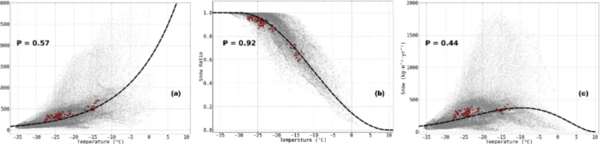
3.2 Solid precipitation

The solid precipitation rate (Ps) can be represented as the product of the total precipi-tation rate (Pt) and the snow-ratio (Sr):

10

Ps₌Pt·Sr (2)

Hence, determining Ps as a function of SAT T is equivalent to establishing statistical relationships between Pt andT, and between Sr andT.

As expected, the large dispersion seen in Fig. 1a confirms that the total precipitation rate Pt does not depend solely onT, but also on the regional atmospheric circulation. 15

According to the Clausius–Clapeyron relation, the saturation water vapour pressure changes exponentially with temperature (Lawrence, 2005), hinting at the mathematical form of Pt (see Appendix). Hence we fit our data with an exponential:

Pt=Pt₀exp(−γ_Pt(T−T_Pt)) (3)

where 20

Pt₀₌2916.0 kg m−2_yr−1

γ_Pt₌0.08◦ C−1

(10)

TCD

7, 3163–3207, 2013

GCM output

M. Geyer et al.

Title Page

Tables Figures

◭ ◮

Back Close

Full Screen / Esc

Discussion

P

a

per

|

D

iscussion

P

a

per

|

Discussion

P

a

per

|

Discuss

ion

P

a

per

|

This statistical relationship is valid for temperatures ranging from about −40◦C to

+10◦

C, the range in which data were available. A linear approximation of the exponent of the Clausius–Clapeyron equation (Appendix A) as a function ofT shows a slope of 0.073◦C−1, which is rather close to the value we obtained for γ_Pt. Boer (1993) and Gregory and Huybrechts (2006) obtained slightly smaller values of 0.065◦

C−1 _and

5

0.05◦C−1, respectively.

Plotting the snow-ratio data against T (Fig. 1b) reveals a well-known oblique step distribution (e.g. Byun et al., 2007). To fit the data, we assume that precipitation falls only as snow for temperatures belowT_Psmin₌−30◦C. Under this condition, the data can then be approximated by the following function

10

Sr=1, T ≤Tmin

Ps

Sr₌0.5 1₊cos π T −T

min Ps

Tmax

Ps −T min Ps

!!

, T_Psmin< T < T_Psmax

Sr=0, T ≥Tmax

Ps

(4)

where

T_Psmin₌−30◦C

T_Psmax_{= +}10◦ C 15

This means that precipitation falls only as rain for annual mean SAT above T_Psmax₌ +10,◦C.

Plotting the annual mean solid precipitation against annual mean SAT (see Fig. 1c) shows that the snowfall rate is largest when the annual mean SAT is between−15◦C 20

and−5◦C, whereas it is small at positive and extreme negative temperatures. A direct fitting of these data by a polynomial fails, as the resulting function is not able to repre-sent a realistic decay of snowfall for positive temperatures. Using Eq. (1), (3) and (4),

(11)

TCD

7, 3163–3207, 2013

GCM output

M. Geyer et al.

Title Page

Tables Figures

◭ ◮

Back Close

Full Screen / Esc

Discussion

P

a

per

|

D

iscussion

P

a

per

|

Discussion

P

a

per

|

Discuss

ion

P

a

per

|

the annual mean Ps can be represented as the following function of the annual mean

T:

Ps=Pt₀exp (−γ_Pt(T−T_Pt)) , Tmin

Ps ≥T

Ps₌0.5 Pt₀exp (−γ_Pt(T−T_Pt)) 1₊cos π T−T

min Ps

Tmax

Ps −T min Ps

!!

, T_Psmin< T < T_Psmax

Ps=0, T_Psmax≤T

(5)

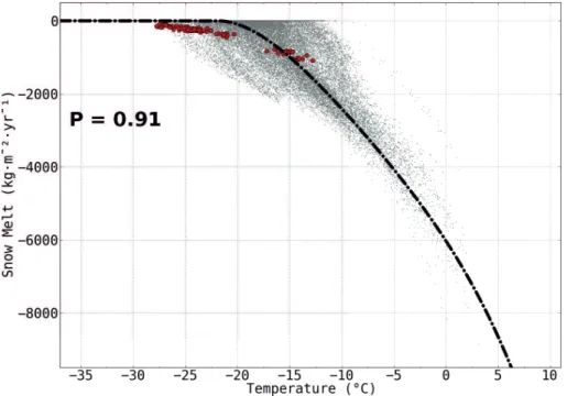
3.3 Snowmelt 5

As expected, Fig. 2 shows that the snowmelt tends to increase with SAT (e.g. Franco et al., 2013). Nevertheless, the dispersion of the scatter plot of snowmelt against tem-perature is rather large, especially when the snowmelt is weak. This is due to the fact that a given negative annual mean SAT may correspond as much to negative daily tem-peratures throughout the year (no snowmelt in this case) as to negative and positive 10

temperatures (some snowmelt is expected). To fit the data with a polynomial we place two constraints: (i) for T ₌−5◦C, the polynomial function should return a snowmelt valueR₌−4000 kg m−2yr−1 and (ii) for temperatures below a critical value T_Rmin, the snowmelt is zero; at this point, the snowmelt function is continuously differentiable, hence its slope is zero. The data are then fitted with a polynomial of degree four: 15

R₌0, T < T_Rmin

(12)

TCD

7, 3163–3207, 2013

GCM output

M. Geyer et al.

Title Page

Tables Figures

◭ ◮

Back Close

Full Screen / Esc

Discussion

P

a

per

|

D

iscussion

P

a

per

|

Discussion

P

a

per

|

Discuss

ion

P

a

per

|

where

T_Rmin₌−21.5◦C

R₀₌−6033.681 kg m−2yr−1

R₁₌−440.911 kg m−2yr−1◦C−1

R₂₌−12.720 kg m−2yr−1◦C−2 5

R₃₌−0.697 kg m−2_yr−1◦ C−3

R₄₌−0.021 kg m−2yr−1◦C−4

Using this function, the snowmelt increases less with temperature than in Franco et al. (2013), where an exponential fit was used. In our case, an exponential fit did 10

not correctly match the data.

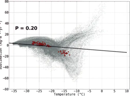
3.4 Sublimation

The annual sublimation data (Fig. 3) does not show any clear relationship to annual mean SAT. This can be explained in part by their strong space variability. Another factor is that our sublimation data aggregates both sublimation itself and condensation. 15

Therefore, for temperatures above−15◦C, the scatter-plot has a “fish-tailed” pattern. Its upward and downward limbs represent condensation and sublimation, respectively. It would be necessary to fit condensation and sublimation separately. However, our database does not include separate estimations of both processes, so we fitted the sum of sublimation and condensation directly. To this end, we use a simple linear fit: 20

Sb=Sb₀+Sb₁T, (7)

where

Sb₀=−9.51 kg m−2yr−1

Sb₁₌−0.36 kg m−2yr−1◦C−1 25

(13)

TCD

7, 3163–3207, 2013

GCM output

M. Geyer et al.

Title Page

Tables Figures

◭ ◮

Back Close

Full Screen / Esc

Discussion

P

a

per

|

D

iscussion

P

a

per

|

Discussion

P

a

per

|

Discuss

ion

P

a

per

|

This function reflects the fact that, on average, under very low SATs, the ice surface tends to condensate air moisture, whereas an increase in SAT favours surface subli-mation. Note that the correlation between the data and the fit is very poor. However, in general the sublimation and condensation processes can be neglected, since they are much smaller than the other terms of the SMB.

5

3.5 Surface mass balance

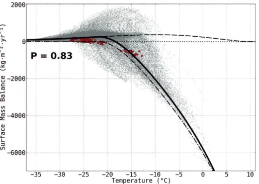
The annual mean SMB data are plotted against SAT in Fig. 4. The sign of the SMB is determined primarily by the sum of solid precipitation and snowmelt. Statistical rela-tionships to temperature have been established for solid precipitation (Eq. 5), snowmelt (Eq. 6) and sublimation (Eq. 7). Their sum yields SMB (Eq. 1). As shown in Fig. 4, the 10

resultingB-function is a correct fit of SMB. This function describes how, on average over the GrIS, the SMB changes as a function of annual mean SAT. It reaches its maximum atT_smbmax≈ −21.7◦C. From this point, it declines slowly with temperature and decreases rapidly as temperature increases. It becomes negative if the annual mean SAT rises above approximately−18.3◦C.

15

In Figs. 1–4 we also plotted the corresponding area-averaged values of the data used in order to compare them with the identified fitted functions. It turns out that these functions also provide reasonable estimations of the GrIS mean mass-balance compo-nents as a function of GrIS mean SAT.

3.6 Downscaling 20

The identified statistical relations allow SMB to be downscaled from the CNRM-CM5.1 150 km-grid to the 15 km grid. To this end, the low-resolution SMB is interpolated from the low to the high resolution grid. This interpolated SMB needs to be corrected to obtain an SMB with realistic spatial variability. We assume that this correction depends on the altitude di_fference between the high-resolution topography field HHR and the 25

(14)

TCD

7, 3163–3207, 2013

GCM output

M. Geyer et al.

Title Page

Tables Figures

◭ ◮

Back Close

Full Screen / Esc

Discussion

P

a

per

|

D

iscussion

P

a

per

|

Discussion

P

a

per

|

Discuss

ion

P

a

per

|

can be written as:

∆B₌∂B

∂H∆H, (8)

where_∆H₌HHR−HLR. Eq. (8) can be rewritten as:

∆B₌∂B ∂T

∂T

∂H∆H. (9)

In Eq. (9), ∂H_∂T is the vertical air temperature lapse rate. Following Fausto et al. (2009), 5

we approximate this quantity with its mean value over Greenland, denoted as lr and equal to −6.309 km◦C−1. Hence, we can approximate the SMB correction implied by downscaling as:

∆B₌1

lr

∂B

∂T∆H. (10)

Since the statistical fit ofB depends strongly on temperature (Fig. 4), the resulting 10

SMB corrections may be very di_fferent in regions with similar_∆H but di_fferent SAT an-nual cycles. In the following section, we will discuss only the impact of the mean SAT on SMB corrections due to altitude changes. Figure 5 illustrates how the SMB, repre-sented by functionB, changes with altitude corrections within±600 m, and how these changes depend on the annual mean SAT. We still assume that a change in altitude 15

implies a change in SAT through the lapse-rate coefficient. As previously seen, the functionBhas a maximum atT_smbmax≈ −21.7◦C. For lower temperatures, there is little or no snowmelt, and SMB changes are therefore mostly due to changes in solid precipi-tation rate. For an annual mean SAT lower thanT_smbmax, an altitude lowering first results in an SMB increase (see curves forT ≤ −22◦C). In this case, the temperature increase 20

leads to more snowfall, overcompensating for the associated snowmelt decrease. How-ever, this is no longer the case if the altitude is lowered further and the SMB starts to decrease. For an annual mean SAT higher thanT_smbmax, a decrease in altitude enhances

(15)

TCD

7, 3163–3207, 2013

GCM output

M. Geyer et al.

Title Page

Tables Figures

◭ ◮

Back Close

Full Screen / Esc

Discussion

P

a

per

|

D

iscussion

P

a

per

|

Discussion

P

a

per

|

Discuss

ion

P

a

per

|

the snowmelt and reduces SMB (see curves forT ≥ −20◦C). This example illustrates that the SMB change with altitude is greatly dependent on the annual mean SAT, which is essential to our SMB downscaling method. Indeed, an altitude correction of−500 m at two locations with annual SATs of−10◦C and−25◦C will lead to SMB changes of −1 and₊0.03 m, respectively.

5

4 Validation of the modelled SMB against observations and MAR simulations

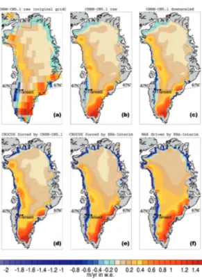
The mean 1989–2008 annual SMB was evaluated by several di_fferent means, as shown in Fig. 6. The original, simply bilinearly interpolated from 150 km to 15 km raw and the downscaled CNRM-CM5.1 SMB are respectively plotted in Fig. 6a–c. The impact of the downscaling is clearly seen along the ice-sheet margins, where SMB is considerably 10

reduced. In contrast, SMB changes are weak in the interior of the GrIS. These changes are consistent with the differences between CNRM-CM5.1’s 150 km resolution topog-raphy and the 15 km resolution topogtopog-raphy (Fig. 7). Moreover, according to Fig. 5, for a given altitude change, the higher the annual SAT, the bigger the SMB correction. This is why the downscaling greatly reduces the SMB, namely at the south-western 15

margin of the GrIS, where the high-resolution topography is significantly lower than its low-resolution counterpart (up to several hundred metres) and the annual mean tem-perature is relatively high. Conversely, in the interior of the GrIS, the low annual mean temperature does not produce large SMB corrections, even where topographic di_ff er-ences are considerable. Another important feature of the downscaling is the following: 20

as seen in Fig. 6b and c, the downscaling results in a decrease in SMB over the south-ern dome of the GriS, where accumulation is very high (up to 2 m yr−1) and snowmelt is very low. Unlike in the margin areas, where a decrease in the downscaled SMB is mostly due to an enhancement in the downscaled snowmelt, a decrease in the down-scaled SMB over this southern dome is due to a decrease in the downdown-scaled solid 25

(16)

TCD

7, 3163–3207, 2013

GCM output

M. Geyer et al.

Title Page

Tables Figures

◭ ◮

Back Close

Full Screen / Esc

Discussion

P

a

per

|

D

iscussion

P

a

per

|

Discussion

P

a

per

|

Discuss

ion

P

a

per

|

The downscaled CNRM-CM5.1 SMB along the margins still does not reach those negative values which are characteristic of the simulations of Crocus forced by CNRM-CM5.1 output atmospheric fields (Fig. 6d). The likely reason for this is the overes-timated snow albedo at the margins in CNRM-CM5.1 (Fig. 8a) relative to Crocus (Fig. 8b). This overestimation is due to the large minimum value assumed over per-5

manent ice in CNRM-CM5.1 (0.8); such a large value does not permit a strong positive feedback between albedo and snowmelt. In contrast, the snow albedo modelled by Cro-cus is much lower at the GrIS margins (Fig. 8b), resulting in enhanced snowmelt. Nev-ertheless, the area-averaged SMB reveals that downscaling eliminates about 70 % of the average difference between the low- and high-resolution SMB. It is 18.3 cm yr−1 (in-10

tegrated value for the whole GrIS is 309 Gt/y) for the raw and 14.4 cm yr−1(243 Gt yr−1) for the downscaled CNRM-CM5.1 SMB, respectively, and 13.1 cm yr−1 (221 Gt yr−1) for Crocus (HIST-RCP8.5 scenarios). All these experiments use outputs from CNRM-CM5.1 and allow us to assess the impact of the technique used to simulate SMB. As a comparison, Crocus forced with ERA-Interim (Figs. 6e, 8c) over the same time pe-15

riod evaluates an SMB of 14.8 cm yr−1 (245 Gt yr−1), which is very close to both the downscaled CNRM-CM5.1 SMB and to the Crocus SMB evaluated on the basis of CNRM-CM5.1 atmospheric output fields. This result is very encouraging for the down-scaling method, since the statistical relationships did not use any information from the ERA-Interim/Crocus simulations.

20

We also compared our results with the SMB evaluated by the RCM MAR driven by ERA-Interim lateral boundary conditions (Figs. 6f, 8d). MAR SMB exhibits a wider band along the western margin of the GrIS with a negative SMB, as well as a stronger snowmelt at this edge. The corresponding area-averaging of MAR SMB yields 16.6 cm yr−1 (275 Gt yr−1). Thus, all the simulations we performed here, as well 25

as those of MAR, produce very close area-average SMB means. They also show similar patterns of SMB spatial distribution over the GrIS, highlighting that the west-ern border of the GrIS has the highest snowmelt. Moreover, our area-averaged SMB evaluations are also very consistent with the SMB range produced by several models

(17)

TCD

7, 3163–3207, 2013

GCM output

M. Geyer et al.

Title Page

Tables Figures

◭ ◮

Back Close

Full Screen / Esc

Discussion

P

a

per

|

D

iscussion

P

a

per

|

Discussion

P

a

per

|

Discuss

ion

P

a

per

|

presented in Rae et al. (2012). This provides strong evidence that the statistical solu-tions found in this work on the basis of Crocus simulasolu-tions are reliable.

Comparison between SMB (Fig. 6) and the corresponding surface albedo (Fig. 8) evaluations shows that snow albedo has a strong feedback on SMB (e.g. Tedesco et al., 2011, 2012). To study this subject more precisely, and in order to assess our 5

SMB simulations along the margins, we use observations from automatic weather sta-tions (AWS) for the period 2000–2010 (Van de Wal et al., 2012). These weather stasta-tions are located on the western part of the GrIS along the K-transect (67◦N). This area is characterized by relatively high ablation (up to 5 m yr−1near the margins) and low ac-cumulation (0.3 m yr−1, Van de Wal et al., 2012). To make a solid representation of the 10

simulated variables along the transect, we average the corresponding values along the 1◦ band centred in 67◦N (from 66.5◦N to 67.5◦N). Cross-sections of CNRM-CM5.1 (150×150 km2), ETOPO1 used in this study as a reference for Crocus (15×15 km2) and MAR (5×5 km2) along the K-transect are shown in Fig. 9a. Both the simulated and the observed SMB are presented in Fig. 9b as a function of surface elevation. As 15

seen, the raw CNRM-CM5.1 SMB is in close agreement with the observations for high altitudes (H >1500 m), but fails in representing the large negative values observed at lower altitudes. As seen from Fig. 9b, relative to CNRM-CM5.1 simulations, the SMB modelled by Crocus is much more consistent with observations. This is especially true when Crocus is forced with ERA-Interim, in spite of the fact that ERA-Interim topog-20

raphy is too smooth, which impacts the quality of its precipitation field. The accuracy of Crocus SMBs is comparable to high-resolution MAR SMB evaluation, which is the closest to the AWS observations (we can also refer for this case to the works from Box et al. (2006) and Krinner and Julien, 2007). Relative to the AWS observations, both Crocus simulations overestimate SMB at lower altitudes, while MAR slightly underesti-25

mates SMB over the entire transect.

(18)

TCD

7, 3163–3207, 2013

GCM output

M. Geyer et al.

Title Page

Tables Figures

◭ ◮

Back Close

Full Screen / Esc

Discussion

P

a

per

|

D

iscussion

P

a

per

|

Discussion

P

a

per

|

Discuss

ion

P

a

per

|

modelled (CNRM-CM5.1, Crocus, MAR) surface snow albedos evaluated along the K-Transect for the summer season are presented in Fig. 9c. We compare them with the corresponding measurements based on the MODerate-resolution Imaging Spec-troradiometer (MODIS). Its observational data is based on 16 day albedo products (MCD43C3), which have been evaluated with respect to field measurements on the 5

GrIS (Stroeve et al., 2005). Their root-mean-square error in comparison with field mea-surements is±0.04 for albedos smaller than 0.07 with high quality flags. The product was reprojected on the same grid as the model, taking great care to remove pixels with low quality flags. We use here the white sky albedos, i.e. the albedo under dif-fuse illumination, to avoid the effect of varying solar zenith angle. All pixels classified 10

as less than 100 % of snow were also removed from the calculation. Due to the fact that low inclinations of the sun may greatly hamper satellite measurements of albedos (Stroeve et al., 2005; Box et al., 2012), only observations for the summer season are considered here. However, the greatest part of the annual GrIS snowmelt occurs in this period (e.g., Tedesco et al., 2011, 2012).

15

As seen in Fig. 9c, the albedo modelled by Crocus is generally in good accordance with the MODIS measurements. MAR and Crocus forced by ERA-Interim produce an inferior albedo relative to the MODIS observations for the high altitudes and conversely for the low altitudes. The albedo is slightly overestimated for Crocus forced by CNRM-CM5.1 atmospheric outputs over the entire transect. These albedos greatly decline 20

with altitude, decreasing from 0.8 for high latitudes to about 0.5 for lower altitudes. At the same time, CNRM-CM5.1 albedo does not go even below 0.8. Comparison of Fig. 9b and c reveals a strong link between the snow albedo and the correspon-dent SMB. Thus, the overestimated values of SMB evaluated by CNRM-CM5.1 or by Crocus/CNRM-CM5.1 relative to the SMB observations are well aligned with the corre-25

sponding overestimation of surface albedo. This suggests that most of the discrepancy between the observations and the downscaled CNRM-CM5.1 SMB is more likely due to the corresponding albedo discrepancy, rather than the downscaling technique.

(19)

TCD

7, 3163–3207, 2013

GCM output

M. Geyer et al.

Title Page

Tables Figures

◭ ◮

Back Close

Full Screen / Esc

Discussion

P

a

per

|

D

iscussion

P

a

per

|

Discussion

P

a

per

|

Discuss

ion

P

a

per

|

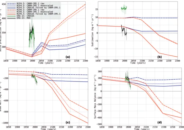
5 SMB future projections

In this section we estimate future SMB changes and how the proposed downscal-ing technique affects SMB under different future climate scenarios. Both RCP4.5 and RCP8.5 future climate scenarios predict a significant SAT rise over the whole GrIS. The two scenarios diverge only after the mid-21st century (Fig. 10). Relative to the end 5

of the 20th century for RCP4.5 (RCP8.5), the annual mean SAT increases by about 2 (5)◦C at the end of the 21st century, 3 (11)◦C at the end of the 22nd century and 3 (12)◦

C at the end of the 23rd century, respectively. As seen, the cold SAT bias over Greenland in CNRM-CM5.1 reaches almost 6◦C relative to the ERA-Interim/Crocus SAT for 1981–2011. In comparison with the ERA-Interim/Crocus SAT, MAR shows 10

much colder temperatures. This may come from MAR’s capacity to perform an ac-tual coupling between a detailed snowpack and the atmosphere, while ERA-Interim may suffer from a poorer representation of the snowpack and a design which does not account for polar physical processes (i.e. cloud microphysics and impacts of stability on turbulent fluxes).

15

The future climate scenarios project a general increase in solid precipitation (Fig. 11a). We see that the downscaling method reduces the solid precipitation. For the past and present climates, the downscaled precipitation becomes more consistent with the corresponding precipitation of Crocus driven by CNRM-CM5.1 atmospheric fields. Obviously, the di_fferent formulations of the definition of solid precipitation in these 20

two models become more significant in the future scenarios and result in a greater dis-agreement between the simulations. Figure 11a also highlights that the amount of solid precipitation is noticeably higher in ERA-Interim (used by Crocus) and MAR than in the HIST-RCP scenarios used. As relatively to ERA-Interim and MAR, HIST-RCP climate scenarios overestimate solid precipitation on the western part of the GrIS south-25

(20)

TCD

7, 3163–3207, 2013

GCM output

M. Geyer et al.

Title Page

Tables Figures

◭ ◮

Back Close

Full Screen / Esc

Discussion

P

a

per

|

D

iscussion

P

a

per

|

Discussion

P

a

per

|

Discuss

ion

P

a

per

|

The simulations we performed reveal a non-significant increase in sublimation (Fig. 11b). Though all the simulations show di_fferent area-averaged sublimation, its values are insignificant in comparison to solid precipitation or to snowmelt.

An intensification of the snowmelt appears in all the climate scenarios considered (Fig. 11c). As seen in this figure, the downscaling considerably enhances the snowmelt, 5

compared with the raw SMB outputs of CNRM-CM. The downscaled CNRM-CM5.1 and Crocus (forced by CNRM-CM5.1 atmospheric forcings) snowmelts are in good agree-ment with ERA-Interim/Crocus and MAR snowmelt until the year 2000. Afterwards, the latter show a much more dramatic snowmelt, which is not the case for the simulations based on HIST-RCP scenarios. This provides further evidence that the CMIP5 models 10

underestimate some of the rapid changes experienced by the Arctic cryosphere over the last decade (e.g. Derksen and Brown, 2012; Stroeve et al., 2012).

SMB, which is greatly affected by snowmelt and by solid precipitation, shows a gen-erally negative trend for the both RCP future climate scenarios through the end of the 21st century (Fig. 11d). Subsequently, under RCP4.5, the mean GrIS SMB stabilises 15

and remains positive, close to+0.1 m yr−1. In contrast, RCP8.5 projects a strong SMB decline after the 21st century due to the large increase in snowmelt. For this scenario, the increase in snowmelt overcompensates for the corresponding increase in solid pre-cipitation, resulting in a negative area-averaged SMB during the 22nd century. At the end of the 23rd century it decreases further, to−0.4 m yr−1.

20

Note that SMB (as well as solid precipitation and snowmelt) evaluations performed by ERA-Interim/Crocus and MAR are in excellent mutual agreement. They both decrease more rapidly after year 2000, when snowmelt enhances precipitously. Nevertheless, for the simulated period 1981–2011, ERA-Interim SMBs always remains positive. Similarly to the snowmelt case, the SMB decrease modelled by CNRM-CM5.1 (and similarly by 25

Crocus forced with CNRM-CM5.1) is much more modest than those of ERA-Interim. Figure 11a–d shows that this underestimation of the recent CNRM-CM5.1 SMB de-crease is due to the underestimation of snowmelt, which can probably be linked to the

(21)

TCD

7, 3163–3207, 2013

GCM output

M. Geyer et al.

Title Page

Tables Figures

◭ ◮

Back Close

Full Screen / Esc

Discussion

P

a

per

|

D

iscussion

P

a

per

|

Discussion

P

a

per

|

Discuss

ion

P

a

per

|

above-mentioned CNRM-CM5.1 cold temperature bias (Fig. 10) and the overestimated summer surface albedo (Figs. 8 and 9c).

As seen from Fig. 11d, downscaling improves the representation of CNRM-CM5.1 SMB, which approaches the SMB evaluated by Crocus. Note, however, that the diff er-ence between the raw and downscaled SMB tends to increase with time. This is due to 5

the fact that the impact of a given altitude correction on SMB increases with SAT, as dis-cussed in Sect. 3.6 (see also Fig. 5), which is the case for both future climate scenarios considered here, but especially for RCP8.5. Conversely, over the period 1850–2000, when SAT changes are weak, the difference between the raw and downscaled SMB is almost constant (Fig. 11d).

10

Crocus forced by CNRM-CM5.1 atmospheric forcings always projects a lower SMB than itself CNRM-CM5.1. As was already shown in Sect. 4, this is probably due to the different snow albedo representations used in these two models. As the lowest snow albedo in CNRM-CM5.1 is prescribed to 0.8, the feedback of surface melting on SMB through a decrease in snow albedo is not represented. In contrast, this feedback 15

plays a major role in Crocus, triggering earlier seasonal snow surface melting and the reappearance of below-the-surface old ice in summer. The latter explains the greater decrease of RCP8.5 Crocus snowmelt (Fig. 11c) and SMB (Fig. 11d) projections for the 21st and 22nd century relative to CNRM-CM5.1 modelling. However, the further contin-uous snowfall augmentation eventually leads to a rise in the average GrIS snow albedo 20

for the 23rd century (not shown here). For Crocus modelling, which simulates the re-freezing of liquid water in the firn in winter, this results in a corresponding decrease of the mean GrIS snowmelt amplification rate due to acceleration of the meltwater re-freeze. This important process, which delays the acceleration of lower SMB values over the higher areas, is not represented in CNRM-CM5.1 (as it does not include the 25

melt-refreeze process).

(22)

TCD

7, 3163–3207, 2013

GCM output

M. Geyer et al.

Title Page

Tables Figures

◭ ◮

Back Close

Full Screen / Esc

Discussion

P

a

per

|

D

iscussion

P

a

per

|

Discussion

P

a

per

|

Discuss

ion

P

a

per

|

the beginning of the 21st century, the ice loss is considerably enhanced at the margins of the GrIS, particularly in the southwest, reaching a rate of more than one metre per year at the end of the 23rd century. The differences between the downscaled and raw SMB for 2001–2010 and 2291–2300 are respectively plotted in Fig. 12b and d. Accord-ing to Eq. (10), these di_fferences are functions of both SAT changes and di_fferences in 5

topography between CNRM-CM5.1 and ETOPO1 (Fig. 7). Since SAT changes are still small in 2001–2010 relative to 1850–1859, the impact of altitude corrections on SMB is notable only at the margins, where altitude corrections are significant (up to several hundred metres). In contrast, since by the end of the 23rd century the SAT increases considerably over the GrIS, the same altitude correction results in a much bigger SMB 10

change, as explained in Sect. 3.6. This is particularly obvious in the area delimited by a box in Fig. 12, where the negative altitude correction is relatively large. In this region, the SMB changes due to downscaling are close to zero at the beginning of the 21st century (Fig. 12b) and reach−0.5 m yr−1by the end of the 23rd century (Fig. 12d).

It is practical to convert GrIS SMB changes relative to 1850–1859 to equivalent global 15

sea level variations. Over the 2001–2010 period, our sea level rise estimation is about

+0.25 mm yr−1, based on CROCUS simulations forced by CNRM-CM5.1 output. This is much lower than recent satellite observations of the total GrIS contribution to sea level rise (GRACE ∼0.7 mm yr−1 in 2006, Rignot et al., 2011; ICESat ∼0.65 mm yr−1 for the period 2003–2008, Sørensen et al., 2011). However, the latter estimations take all 20

types of mass loss (SMB, ice calving, basal melt) into account, whereas our estimations are based only on SMB anomalies. As seen in Fig. 13a, the projected sea level rise rate computed from Crocus SMB anomalies is almost doubled (0.4 mm yr−1, RCP4.5) and quadrupled (0.8 mm yr−1_{, RCP8.5) for 2100. This corresponds to about 3 (RCP4.5)}

and 4.5 cm (RCP8.5) of absolute sea level rise for the 21st century (Fig. 13b). These 25

results are in agreement with Huybrechts et al. (2004), Oerlemans et al. (2005), Meehl et al. (2007), Fettweis et al. (2008), where close estimations of sea level rise based on GrIS SMB anomalies were projected for the A1B scenario. However, our results are underestimated relative to 4±2 cm and 9±4 cm for the same RCP 4.5 and RCP 8.5

(23)

TCD

7, 3163–3207, 2013

GCM output

M. Geyer et al.

Title Page

Tables Figures

◭ ◮

Back Close

Full Screen / Esc

Discussion

P

a

per

|

D

iscussion

P

a

per

|

Discussion

P

a

per

|

Discuss

ion

P

a

per

|

scenarios, respectively, as modelled by Fettweis et al. (2012) on the basis of the RCM MAR. Our underestimation may be due partially to the fact that we used only several 10 yr snapshots of the CNRM-CM5.1 simulations and did not run the entire time period. In any case, as was already shown above, the CNRM-CM5.1 model under HIST-RCP climate scenarios is not capable of fully capturing the ongoing rapid changes occurring 5

over the GrIS for the last decade.

At the end of the 23rd century, with reference to 1850, our Crocus SMB anoma-lies project 0.4 (2.5) mm yr−1of sea level rise rate and 13.5 (46) cm absolute sea level rise for the scenario RCP4.5 (RCP8.5). The downscaled CNRM-CM5.1 SMBs produce stronger SMB anomalies than the raw SMB and, as a consequence, higher sea level 10

rise estimations. The downscaling tends to reduce the di_fference in sea level rise be-tween estimations based on CNRM-CM5.1 and Crocus. For the recent past and the present climate, this effect does not seem to play a significant role in the correspond-ing SMBanomalies, and as a consequence, in the corresponding sea level variations. However, the downscaling acts distinguishably on SMB anomalies with climate warm-15

ing. For example, as seen in Fig. 13b, by the end of 23rd century the downscaling gains an additional 3 and 8 cm of absolute sea level rise for the RCP4.5 and RCP8.5 scenarios, respectively.

It should be noted that the GrIS topography is fixed during our simulations. Therefore, the snowmelt/elevation feedback (Gregory and Huybrechts, 2006) is not considered 20

here. As was shown in Helsen et al. (2012), this feedback amplifies the snowmelt ac-cording to the lapse-rate temperature increment when the surface elevation decreases. This means that our evaluations of the GrIS SMB changes are likely underestimated.

6 Discussion and conclusions

The main goal of SMB downscaling is to turn low-resolution GCM output fields over 25

(24)

TCD

7, 3163–3207, 2013

GCM output

M. Geyer et al.

Title Page

Tables Figures

◭ ◮

Back Close

Full Screen / Esc

Discussion

P

a

per

|

D

iscussion

P

a

per

|

Discussion

P

a

per

|

Discuss

ion

P

a

per

|

downscaling is applied to compute SMB corrections as a function of altitude changes between the coarse and fine grids. In this study, the corrections are computed on an annual basis. To do so, we determined statistical relationships between SAT changes and the changes in the different components of SMB, and assumed that a SAT change is linked to an altitude change through a constant lapse-rate. For the recent past (1981– 5

2011), Crocus simulations (HIST-RCP climate scenarios), which form the basis for sta-tistical relationships, are in good agreement with the available high-resolution simula-tions of MAR driven by ERA-Interim lateral boundary condisimula-tions. This provides sound evidence that the statistical solutions found here are reliable.

The developed downscaling technique offers an improved SMB over most of the 10

GrIS, taking into account changes in small-scale topography. However, it may intro-duce smoothing effects, since we chose to fit annual mean data with functions of one variable, namely annual mean SAT. The data presents dispersion that can be due ei-ther mostly to di_fferent SAT annual cycles or spatial variability. In the case of snowmelt, a given annual mean SAT can correspond to very di_fferent SAT annual cycles, and 15

hence very different snowmelts. Thus the annual mean SAT alone is not the best pre-dictor for annual mean snowmelt. Multiple regression on the basis of monthly data may be considered (Such an attempt, not shown here, was made. It demonstrated an expected decrease of the dispersion of the data). Using positive degree-days as a sec-ond predictor in addition to annual mean SAT would be a possibility. In the case of 20

precipitation, spatial variability prevails, contributing significantly to scattering the data. Precipitation is one of the components of the Earth’s complex hydrological cycle. It is connected to SAT, but also depends heavily on a variety of other di_fferent physical characteristics (humidity convergence, solar radiation, etc). A multiple regression of annual mean precipitation based on monthly SAT data would probably not be useful in 25

this case (such an attempt, not shown here, was made. It demonstrated no decrease of the dispersion of the data) and other additional predictors should be found. There-fore, we conclude that although multiple regressions are powerful tools for establishing more reliable statistical laws between snowmelt, precipitation and SAT, they detract

(25)

TCD

7, 3163–3207, 2013

GCM output

M. Geyer et al.

Title Page

Tables Figures

◭ ◮

Back Close

Full Screen / Esc

Discussion

P

a

per

|

D

iscussion

P

a

per

|

Discussion

P

a

per

|

Discuss

ion

P

a

per

|

significantly from the simplicity of the procedure, contrary to one of the objectives of this work.

The downscaling technique we developed results in a general decrease of SMB along the ice sheet margins, mostly because of the snowmelt enhancement. As was shown, the di_fferences between the raw and downscaled SMB tend to increase with 5

SAT. For high temperatures, a given altitude decrease results in a stronger snowmelt amplification than for low temperatures. We noted that the representation of snow albedo by CNRM-CM5.1 is not realistic. However, this does not actually a_ffect the re-lationships found, as the latter were established on the basis of the high-resolution Crocus modelling. A positive outcome from our downscaling technique is that it re-10

duces the discrepancy in GrIS-averaged SMB between raw CNRM-CM5.1 and Crocus SMB by about 70 %. As a result, the downscaled low-resolution CNRM-CM5.1 SMB be-comes very consistent with high-resolution MAR SMB, which opens very encouraging perspectives for the developed technique.

For future climate projections of the GrIS topography’s response to upcoming cli-15

mate change and the consequent impact on sea level rise, it is also important to take into account the feedback between changes in GrIS geometry and SMB (Gregory and Huybrechts, 2006; Helsen et al., 2012). Currently, most global and regional atmo-sphere/surface climate models do not modify topography online. However, it is possible to account for the impact of GrIS topography changes on SMB as such models are run 20

if these changes are small enough not to a_ffect atmospheric circulation significantly. Assuming this, the SMB can be corrected online following our downscaling technique.

Appendix

An approximation of the Clausius–Clapeyron equation

A good approximation of the Clausius–Clapeyron relation providing the saturation 25

(26)

TCD

7, 3163–3207, 2013

GCM output

M. Geyer et al.

Title Page

Tables Figures

◭ ◮

Back Close

Full Screen / Esc

Discussion

P

a

per

|

D

iscussion

P

a

per

|

Discussion

P

a

per

|

Discuss

ion

P

a

per

|

August–Roche–Magnus formula (Lawrence, 2005):

P(T)=P₀exp _aT

T₊b

,

where

P₀₌6.1094 hPa

a₌17.625 5

b₌243.04

c₌−12.75◦C

P(T) is the equilibrium or saturation vapour pressure as a function of temperatureT on the Celsius scale. The equation can be further approximated by linearizing the expo-10

nent:

P(T)=P₀exp a

bT

1 1+T_b

!

=P₀exp _a

bT

1−1

bT+. . .

≈P₀exp (γ₀T) ,

whereγ₀₌a_b≈0.073. For values ofT typically ranging from−50 to 50◦C, the maximum approximation error of the final formulation is 20 %. Assuming snow accumulationP s

is itself linearly linked to the saturation vapour pressure, this justifies that within the 15

considered temperature interval, theP s(T) function can be broadly approximated with an exponential with a linear argument.

Acknowledgements. The authors thank Xavier Fettweis for providing the MARv3.2 outputs. The authors are also grateful to Aurélien Ribes for useful discussion and propositions concerning the applied statistics. We would especially like to thank Aurore Voldoire for

20

her constant support throughout this work. We also owe our gratitude to all the others colleges who helped us at different stages of the work. This work was funded by the Euro-pean Commission’s 7th Framework Programme, under Grant Agreement number 226520,

(27)

TCD

7, 3163–3207, 2013

GCM output

M. Geyer et al.

Title Page

Tables Figures

◭ ◮

Back Close

Full Screen / Esc

Discussion

P

a

per

|

D

iscussion

P

a

per

|

Discussion

P

a

per

|

Discuss

ion

P

a

per

|

COMBINE project. The authors also acknowledge the support of Météo-France, CNRS and the French Agence Nationale de la Recherche (ANR) under reference ANR-09-CEP-001-01 (CECILE project). Figures were created using the NCL, matplotlib and CDAT graphic packages.

The publication of this article is financed by CNRS-INSU.

5

References

Amante, C. and Eakins, B. W.: ETOPO1 1 Arc-Minute Global Relief Model: Procedures, Data Sources and Analysis, NOAA Technical Memorandum NESDIS NGDC-24, 19 pp., March 2009.

Bamber, J. L., Griggs, J. A., Hurkmans, R. T. W. L., Dowdeswell, J. A., Gogineni, S. P., Howat, I.,

10

Mouginot, J., Paden, J., Palmer, S., Rignot, E., and Steinhage, D.: A new bed elevation dataset for Greenland, The Cryosphere, 7, 499–510, doi:10.5194/tc-7-499-2013, 2013. Bengtsson, L., Koumoutsaris, S., and Hodges, K.: Large-scale surface mass balance of

ice sheets from a comprehensive atmospheric model, Surv. Geophys., 32, 459–474, doi:10.1007/s10712-011-9120–8, 2011.

15

Boer, G. J.: Climate change and the regulation of the surface moisture and energy budgets, Clim. Dynam., 8, 225–239, 1993.

Bougamont, M., Bamber, J. L., Ridley, J. K., Gladstone, R. M., Greuell, W., Hanna, E., Payne, A. J., and Rutt, I.: Impact of model physics on estimating the surface mass balance of the Greenland ice sheet, Geophys. Res. Lett., 34, L17501, doi:10.1029/2007GL030700,

20

2007.

(28)

TCD

7, 3163–3207, 2013

GCM output

M. Geyer et al.

Title Page

Tables Figures

◭ ◮

Back Close

Full Screen / Esc

Discussion

P

a

per

|

D

iscussion

P

a

per

|

Discussion

P

a

per

|

Discuss

ion

P

a

per

|

Box, J. E., Bromwich, D. H., Veenhuis, B. A., Bai, L.-S., Stroeve, J. C., Rogers, J. C., Steffen, K., Haran, T., and Wang, S.-H.:, Greenland Ice Sheet surface mass balance variability (1988– 2004) from calibrated Polar MM5 output, J. Climate, 19, 2783–2800, 2006.

Box, J. E., Fettweis, X., Stroeve, J. C., Tedesco, M., Hall, D. K., and Steffen, K.: Greenland ice sheet albedo feedback: thermodynamics and atmospheric drivers, The Cryosphere, 6,

5

821–839, doi:10.5194/tc-6-821-2012, 2012.

Brun, E., David, P., Sudul, M., and Brunot, G.: A numerical model to simulate snow-cover stratig-raphy for operational avalanche forecasting, J. Glaciol., 38, 13–22, 1992.

Byun, K.-Y., Yang, J., and T.-Y. Lee: A snow-ratio equation and its application to numerical snowfall prediction, Weather Forecast., 23, 644–658, 2008

10

Cosgrove, B. A., Lohmann, D., Mitchell, K. E., Houser, P. E., Wood, E. F., Schaake, J., Robock, A., Marshall, C., Sheffield, C., Luo, L., Duan, Q., Pinker, R., T., Tarpley, J., D., Higgins, R. W., and Meng. J.: Real-time and retrospective forcing in the North Amer-ican Land Data Assimilation System (NLDAS) project, J. Geophys. Res., 108, 8842, doi:10.1029/2002JD003118, 2003.

15

Dee, D. P., Uppala, S. M., Simmons, A. J., Berrisford, P., Poli, P., Kobayashi, S., Andrae, U., Balmaseda, M. A., Balsamo, G., Bauer, P., Bechtold, P., Beljaars, A. C. M., van de Berg, L., Bidlot, J., Bormann, N., Delsol, C., Dragani, R., Fuentes, M., Geer, A. J., Haimberger, L., Healy, S. B., Hersbach, H., Hólm, E. V., Isaksen, L., Kållberg, P., Köhler, M., Matricardi, M., McNally, A. P., Monge-Sanz, B. M., Morcrette, J.-J., Park, B.-K., Peubey, C., de Rosnay, P.,

20

Tavolato, C., Thépaut, J.-N., and Vitart, F.: The ERA-Interim reanalysis: configuration and performance of the data assimilation system, Q. J. Roy. Meteorol. Soc., 137, 553–597, doi:10.1002/qj.828, 2011.

Derksen, C. and Brown, R.: Spring snow cover extent reductions in the 2008– 2012 period exceeding climate model projections, Geophys. Res. Lett., 39, L19504,

25

doi:10.1029/2012GL053387, 2012.

Ettema, J., van den Broeke, M. R., van Meijgaard, E., van de Berg, W. J., Bamber, J. L., Box, J. E., and Bales, R. C.: Higher surface mass balance of the Greenland ice sheet revealed by high-resolution climate modelling, Geophys. Res. Lett., 36, L12501, doi:10.1029/2009GL038110, 2009.

30

Fausto, R. S., Ahlstrøm, A. P., van As, D., Bøggild, C. E., and Johnsen, S. J.: A new present-day temperature parameterization for Greenland, J. Glaciol., 55, 95–105, doi:10.3189/002214309788608985, 2009.