ACPD
10, 19005–19029, 2010Effectiveness of the Montreal Protocol to
protect the ozone layer
J. A. M ¨ader et al.
Title Page
Abstract Introduction
Conclusions References
Tables Figures
◭ ◮
◭ ◮
Back Close
Full Screen / Esc
Printer-friendly Version
Interactive Discussion
Discussion
P
a
per
|
Dis
cussion
P
a
per
|
Discussion
P
a
per
|
Discussio
n
P
a
per
|
Atmos. Chem. Phys. Discuss., 10, 19005–19029, 2010 www.atmos-chem-phys-discuss.net/10/19005/2010/ doi:10.5194/acpd-10-19005-2010
© Author(s) 2010. CC Attribution 3.0 License.
Atmospheric Chemistry and Physics Discussions
This discussion paper is/has been under review for the journal Atmospheric Chemistry and Physics (ACP). Please refer to the corresponding final paper in ACP if available.
Evidence for the e
ff
ectiveness of the
Montreal Protocol to protect the ozone
layer
J. A. M ¨ader1, J. Staehelin1, T. Peter1, D. Brunner1,*, H. E. Rieder1, and W. A. Stahel2
1
Institute for Atmospheric and Climate Science, ETH Zurich, 8092 Zurich, Switzerland 2
Seminar for Statistics, ETH Zurich, 8092 Zurich, Switzerland *
now at: EMPA – Material Science and Technology, Duebendorf, Switzerland
Received: 18 June 2010 – Accepted: 2 August 2010 – Published: 11 August 2010
Correspondence to: J. A. M ¨ader ([email protected])
ACPD
10, 19005–19029, 2010Effectiveness of the Montreal Protocol to
protect the ozone layer
J. A. M ¨ader et al.
Title Page
Abstract Introduction
Conclusions References
Tables Figures
◭ ◮
◭ ◮
Back Close
Full Screen / Esc
Printer-friendly Version
Interactive Discussion
Discussion
P
a
per
|
Dis
cussion
P
a
per
|
Discussion
P
a
per
|
Discussio
n
P
a
per
|
Abstract
The release of man-made ozone depleting substances (ODS, including chlorofluoro-carbons and halons) into the atmosphere has lead to a near-linear increase in strato-spheric halogen loading since the early 1970s, which started to level offafter the mid-1990s and then to decline, in response to the ban of many ODSs by the Montreal 5
Protocol (1987). We developed a multiple linear regression model to test whether this has already a measurable effect on total ozone values observed by the global network of ground-based instruments. The model includes explanatory variables describing the influence of various modes of dynamical variability and of volcanic eruptions. In order to describe the anthropogenic influence a first version of the model contains a linear 10
trend (LT) term, whereas a second version contains a term describing the evolution of equivalent effective stratospheric chlorine (EESC). By comparing the explained vari-ance of these two models we evaluated which of the two terms better describes the observed ozone evolution. For a significant majority of the stations, the EESC proxy fits the long term ozone evolution better than the linear trend term. Therefore, we con-15
clude that the Montreal Protocol has started to show measurable effects on the ozone layer about twenty years after it became legally binding.
1 Introduction
Stratospheric ozone depletion by chlorine radicals was first discussed by Stolarski and Cicerone (1974) and Molina and Rowland (1974). The latter also discovered that man 20
made chlorofluorocarbons (CFCs) act as a source for stratospheric chlorine. The full extent of anthropogenic ozone destruction became evident when the Antarctic ozone hole was discovered (Farman et al., 1985), which was subsequently explained as caused by ozone depleting substances (ODS) including CFCs and halons and a com-plex chemistry involving heterogeneous reactions on the cold surfaces of polar strato-25
ACPD
10, 19005–19029, 2010Effectiveness of the Montreal Protocol to
protect the ozone layer
J. A. M ¨ader et al.
Title Page
Abstract Introduction
Conclusions References
Tables Figures
◭ ◮
◭ ◮
Back Close
Full Screen / Esc
Printer-friendly Version
Interactive Discussion
Discussion
P
a
per
|
Dis
cussion
P
a
per
|
Discussion
P
a
per
|
Discussio
n
P
a
per
|
At northern mid-latitudes, significant negative trends in wintertime total ozone were first documented by the International Ozone Trends Panel (WMO, 1989). Many further studies confirmed a significant decrease in the thickness of the extratropical ozone layer (e.g., Staehelin et al., 2001, 2002).
An efficient reduction of the global anthropogenic emissions of ODS was reached 5
by the Montreal Protocol (1987) and its subsequent Amendments (WMO, 2007). This was confirmed by long-term measurements of selected CFCs at remote ground sta-tions (Montzka et al., 1996) as well as by balloon-borne measurements in the strato-sphere (Engel et al., 2002). The successful implementation of the Montreal Protocol (e.g., WMO, 2007) launched a discussion on ozone recovery in the second half of 10
this century and a potential subsequent super-recovery by greenhouse gas-induced cooling of the upper stratosphere and an predicted increase in the Brewer-Dobson cir-culation as a result of climate change (e.g., Butchart and Scaife, 2001; Newchurch et al., 2003; Krizan et al., 2005; Austin and Wilson, 2006; Butchart et al., 2006; Eyring et al., 2007; Harris et al., 2008; Shepherd, 2008; Hegglin and Shepherd, 2009; Li et 15
al., 2009; McLandress and Shepherd, 2009; Waugh et al., 2009). However, results of numerical simulations published by Hegglin and Shepherd (2009) predicted remark-able differences in the evolution of the ozone layer in the Northern and the Southern Hemisphere within the current century.
Depending on their physico-chemical properties individual ODS have different po-20
tentials to deplete stratospheric ozone. Equivalent Effective Stratospheric Chlorine (EESC) is a convenient quantity to characterize the ozone depletion potentials of halo-gens (chlorine and bromine) taking into account the temporal evolution of the emissions of the individual species, their transport into the stratosphere and their atmospheric lifetimes (WMO, 2007). Since air is transported from the tropical troposphere into the 25
ACPD
10, 19005–19029, 2010Effectiveness of the Montreal Protocol to
protect the ozone layer
J. A. M ¨ader et al.
Title Page
Abstract Introduction
Conclusions References
Tables Figures
◭ ◮
◭ ◮
Back Close
Full Screen / Esc
Printer-friendly Version
Interactive Discussion
Discussion
P
a
per
|
Dis
cussion
P
a
per
|
Discussion
P
a
per
|
Discussio
n
P
a
per
|
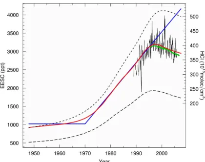
several years after the peak in emissions, due to the long transport time to reach the ozone layer and the long atmospheric lifetimes of ODS. This was confirmed by ground based Fourier Transform Infrared Reflectance (FTIR) measurements at Jungfraujoch (Switzerland) of column amounts of the stratospheric reservoir species hydrogen chlo-ride (HCl), which is formed by the reaction of methane (CH4) with chlorine radicals 5
released by the stratospheric photolysis of CFCs (black line in Fig. 1) (Rinsland et al., 2003). These findings suggest that the slow recovery of the ozone layer over mid-latitudes may have started at the earliest in the late 1990s.
The bulk of stratospheric ozone resides in the lower and middle stratosphere. At these altitudes extra-tropical ozone is highly variable and therefore the effect of the 10
Montreal Protocol on total ozone is much more difficult to identify than in the upper stratosphere (e.g., Weatherhead et al., 2000). Reinsel and colleagues (2002) esti-mated that detection of the first stage of recovery (defined as a deviation from a linear increase) requires about 7–8 years of total ozone observations since the onset of the recovery. Recent studies provide growing evidence that a weakening or reversal of 15
negative trends may already be detectable (Newchurch et al., 2003; Guillas et al., 2004; Steinbrecht et al., 2004; Reinsel et al., 2005; Yang et al., 2005; Brunner et al., 2006; Weatherhead and Anderson, 2006; Yang et al., 2006; WMO, 2007; Harris et al., 2008). Increases in total ozone since the early 1990s have been observed at many sites in northern mid-latitudes, but the attribution of this increase to changes in EESC 20
is a difficult task (Yang et al., 2006) because several factors may have contributed to an apparent flattening or reversal in ozone tendencies, including: (i) changes in synoptic scale meteorological variability and long-term climate variability (e.g., Hood and Zaff, 1995; Steinbrecht et al., 1998; Appenzeller et al., 2000; Thompson an Wallace, 2000; Orsolini and Doblas-Reyes, 2003; Br ¨onnimann and Hood, 2003; Shepherd et al., 2008; 25
ACPD
10, 19005–19029, 2010Effectiveness of the Montreal Protocol to
protect the ozone layer
J. A. M ¨ader et al.
Title Page
Abstract Introduction
Conclusions References
Tables Figures
◭ ◮
◭ ◮
Back Close
Full Screen / Esc
Printer-friendly Version
Interactive Discussion
Discussion
P
a
per
|
Dis
cussion
P
a
per
|
Discussion
P
a
per
|
Discussio
n
P
a
per
|
winters with enhanced polar ozone loss in the Arctic during the mid 1990s and in the Antarctic in 2006 with one of the largest austral ozone holes ever (WMO, 2006).
Numerical simulations have been performed in order to describe in a quantitative way the effect of anthropogenic emissions of ODS on the stratospheric ozone layer. During the last decade a number of three dimensional models have been developed 5
aiming at describing the complex interactions of stratospheric chemistry and transport allowing climatic changes to be taken into account (e.g., WMO, 2007). However, the validation of these models regarding their capability to adequately describe all relevant processes and hence to reliably predict the evolution of stratospheric ozone remains a challenging task (Eyring et al., 2007).
10
Here we use a statistical test as a complementary method to provide evidence for the effectiveness of the Montreal Protocol. The basic concept of the approach is sim-ple: We test whether the temporal evolution of total ozone measurements can be better described by a linear trend (LT, starting on 1 January 1970, as expected without the regulation by the Montreal Protocol), or by the evolution of EESC (including the regula-15
tion; see Fig. 1). The test itself is a binomial test with a probability of 50% (also known as sign-test). The decision between LT and EESC is based on the comparison of the variances (R2) produced by the two versions of the regression model. The model includes additional explanatory variables describing other (natural) influences, which have been previously selected by backward elimination methods. Section 2 contains 20
ACPD
10, 19005–19029, 2010Effectiveness of the Montreal Protocol to
protect the ozone layer
J. A. M ¨ader et al.
Title Page
Abstract Introduction
Conclusions References
Tables Figures
◭ ◮
◭ ◮
Back Close
Full Screen / Esc
Printer-friendly Version
Interactive Discussion
Discussion
P
a
per
|
Dis
cussion
P
a
per
|
Discussion
P
a
per
|
Discussio
n
P
a
per
|
2 Methods and measurements
2.1 Multiple linear regression models and selection of explanatory variables
We used the following multiple regression modelling approach, which describes the explained variance (R2)
TOZ=M+b1·Trend+
m X
j=2
bj·Xj+ε , (1)
5
where “TOZ” is the measured total ozone monthly mean value,M is the seasonal vari-ation of total ozone described by individual values for each month, “Trend” is either EESC or LT,b1the trend coefficient,Xj are other explanatory variables andbj their re-spective coefficients (see Table 1 and text below). The residual errors are described by ε. The autocorrelation (in time) is not taken into account in either versions (using EESC 10
or LT). However, autocorrelation is expected to not affect the results of our comparative analysis, as it should affect both versions in the same way.
The most suitable explanatory variables (describing most of the variance) are se-lected by backward elimination (for a detailed description see M ¨ader et al., 2007). We first selected the explanatory variables for individual stations. We start with a multiple 15
linear regression model including 44 potentially relevant explanatory variables. The significance (p value) of the coefficients is used to eliminate the least important term in the model. With the resulting reduction in variables the step is repeated iteratively until no explanatory variable is left. The sequence of elimination defines a ranking of the variables separately for each station.
20
ACPD
10, 19005–19029, 2010Effectiveness of the Montreal Protocol to
protect the ozone layer
J. A. M ¨ader et al.
Title Page
Abstract Introduction
Conclusions References
Tables Figures
◭ ◮
◭ ◮
Back Close
Full Screen / Esc
Printer-friendly Version
Interactive Discussion
Discussion
P
a
per
|
Dis
cussion
P
a
per
|
Discussion
P
a
per
|
Discussio
n
P
a
per
|
of variables is based on this ranking table, and the number of variables in the model is determined by the number of significant variables and the explained variance (R2) as described in M ¨ader et al. (2007). If not already present, a term for the trend was added.
In the next step, we test, based onR2, whether the temporal evolution of the individ-5
ual stations is better fitted by EESC or by the linear trend LT. Then we calculate, using the sign-test, for the different latitude belts if a significant part of the stations show the same preference. This approach with two comparable proxies for the anthropogenic influence is only qualitative in nature, but it is robust and avoids the selection of a fixed point in time for the turnaround (Percival and Rothrock, 2005) as was done in other 10
studies (Reinsel et al., 2002; Newchurch et al., 2003; Reinsel et al., 2005; Yang et al., 2005; Weatherhead and Anderson, 2006; Yang et al., 2006).
2.2 Spatial correlation
Since the distances between some of the ground-based stations are small, their pref-erence for either EESC or LT may not be independent because of spatial correlations 15
of the measurements. Therefore, we tested the spatial correlation of our results as ex-pressed by the following transformed differenceT between the proportions of explained variance:
T=signREESC2 −R2
LT
·
r R
2
EESC−R 2 LT
(2)
whereREESC2 and RLT2 are the explained variances of the model using either EESC or 20
ACPD
10, 19005–19029, 2010Effectiveness of the Montreal Protocol to
protect the ozone layer
J. A. M ¨ader et al.
Title Page
Abstract Introduction
Conclusions References
Tables Figures
◭ ◮
◭ ◮
Back Close
Full Screen / Esc
Printer-friendly Version
Interactive Discussion
Discussion
P
a
per
|
Dis
cussion
P
a
per
|
Discussion
P
a
per
|
Discussio
n
P
a
per
|
used) is defined as
sC(h)=
1 nC(h)
P
(i ,j)∈h
q Ti−Tj
!4
0.914+0.988nC(h)
(3)
wherenC(h) is the number of pairs of stations in this distance class. Graphs of sC(h) versus h show the structure of the spatial correlation. In case of significant spatial correlations,sC(h)increases withh. Often the increase is restricted to short distances 5
andsC(h) remains constant above a certain distance called range. Above this range, the individual stations are no longer correlated (Cressie, 1993). In our analysis, we calculated the spatial correlation separately for the northern, southern and tropical latitude belt as well as for all stations together (see Sect. 3.1).
2.3 Total ozone measurements used in this study
10
For the ozone time series we used the ground based stations provided by WOUDC (World Ozone and Ultraviolet Data Centre, Toronto, www.woudc.org, measurements up to March 2007 as available in May 2007) with sufficiently long time series (at least 120 monthly mean values and measurements beyond the year 2000). Available series are different in length. Data before 1948 were not used, since the relevant proxies are 15
not available for the time before 1948. However, this restriction affected only a few stations as most ozone time series started later. Ground based measurements were selected because at many stations, observation started in the 1960s or early 1970s, allowing to better fit the individual coefficients of the model (especially for slowly vary-ing processes) than would be possible for satellite observations available since 1979. 20
ACPD
10, 19005–19029, 2010Effectiveness of the Montreal Protocol to
protect the ozone layer
J. A. M ¨ader et al.
Title Page
Abstract Introduction
Conclusions References
Tables Figures
◭ ◮
◭ ◮
Back Close
Full Screen / Esc
Printer-friendly Version
Interactive Discussion
Discussion
P
a
per
|
Dis
cussion
P
a
per
|
Discussion
P
a
per
|
Discussio
n
P
a
per
|
after visual inspection. Under the assumption that data quality problems of individual stations are random, the conclusions drawn here will remain valid, and any further at-tempt to homogenize, improve or select certain data is inevitably connected with other problems or biases.
Totally 116 stations with 34 923 monthly total ozone values were used, which corre-5
sponds to typically 23.5 years of data per station.
3 Results and discussion
3.1 Selected explanatory variables and spatial correlation
The explanatory variables Xj were selected by backward elimination (see Sect. 2.1), starting with a large set of different time series of possible variables. Table 1 shows the 10
result and gives a short description of the selected variables. The variable of equiva-lent latitude (EL) was developed to describe the effect of dynamics on column ozone (Wohltmann et al., 2005). It is based on the equivalent latitude fields of potential vortic-ity vertically integrated using a climatological ozone profile. The EL was selected in all bands except at the South Polar sites. It is known that changes in atmospheric dynam-15
ics contributed significantly to the past evolution of stratospheric ozone at different sites (e.g., Labitzke and van Loon, 1999; Chipperfield and Jones 1999; Appenzeller et al., 2000; Hadjinicolaou et al., 2002; Orsolini and Doblas-Reyes, 2003; Harris et al., 2008) and it is well know that the increase in total ozone found at northern mid-latitudes in the 1990s (Hood and Soukharev, 2005; Harris et al., 2008) is attributable to a large extent 20
to changes in dynamics. The inclusion of EL in the model gives some confidence that the main results of the study are not confused by changes in dynamics, since changes in transport are believed to be the main driver for the long-term evolution of the ozone shield besides ODS.
A large perturbation of stratospheric ozone was caused by the eruption of Mount 25
ACPD
10, 19005–19029, 2010Effectiveness of the Montreal Protocol to
protect the ozone layer
J. A. M ¨ader et al.
Title Page
Abstract Introduction
Conclusions References
Tables Figures
◭ ◮
◭ ◮
Back Close
Full Screen / Esc
Printer-friendly Version
Interactive Discussion
Discussion
P
a
per
|
Dis
cussion
P
a
per
|
Discussion
P
a
per
|
Discussio
n
P
a
per
|
to lower total ozone values in the subsequent years (e.g., Randel et al., 1995; Hadjini-colaou et al., 1997), this may lead to a preference for EESC over the linear trend. Based on the backward elimination procedure the variable SAD (vertically integrated strato-spheric aerosol surface area density) representing the effect of volcanic eruptions was identified as an essential variable in the two northern latitude belts. On the Southern 5
Hemisphere the influence of the past volcanic eruptions (e.g., Gunung Agung, 1963; El Chich ´on, 1982; Mt. Pinatubo, 1991) on column ozone could not be identified in similar strength as in the Northern Hemisphere. This hemispheric difference in the effect of volcanic eruptions was explained by Robock et al. (2007) as the combination of the difference in land mass at the latitude of the jet stream and the stronger polar vortex in 10
the Southern Hemisphere. The inclusion of SAD in the model distinctively reduces the residuals for the corresponding time period. Thus, in contrast to other studies (Rein-sel et al., 2002; Yang et al., 2006) we apply the regression model including SAD to the complete ozone time series instead of removing a couple of years following the eruption of Mount Pinatubo.
15
In earlier WMO assessments the Quasi Biennial Oscillation (QBO) and the eleven year solar cycle were used as explanatory variables in order to remove long-term vari-ability in statistical trend models. They were not selected as important proxies for the long-term ozone evolution in our model selection procedure (comp. M ¨ader et al., 2007). Possibly some of the variability caused by QBO is captured by EL. The solar cycle is 20
nevertheless included as explanatory variable in the sensitivity analysis presented in Sect. 3.2.
To illustrate the model performance one sample station for the Northern mid-latitude (Hohenpeissenberg, Germany) and the Northern Polar belt (Resolute, Canada) is an-alyzed (see supplementary material).
25
ACPD
10, 19005–19029, 2010Effectiveness of the Montreal Protocol to
protect the ozone layer
J. A. M ¨ader et al.
Title Page
Abstract Introduction
Conclusions References
Tables Figures
◭ ◮
◭ ◮
Back Close
Full Screen / Esc
Printer-friendly Version
Interactive Discussion
Discussion
P
a
per
|
Dis
cussion
P
a
per
|
Discussion
P
a
per
|
Discussio
n
P
a
per
|
global). But for the single belts no increase insC(h) even for small distances is visible, but rather,sC(h) appears to stay constant (this situation is called apure-nugget-model and implies uncorrelated random deviations). Therefore we may assume that spatial correlation does not reduce the multitude of pieces of independent information in our test, as long as we analyze the three latitude belts separately.
5
3.2 Long-term ozone evolution: linear trend vs. EESC
After selection of the explanatory variables for each latitudinal belt a test was used to study whether the measurements of the individual sites rather follow a linear trend or the time evolution of EESC (see also introduction). The trend term was estimated for every calendar season separately and a binomial test was used to test whether 10
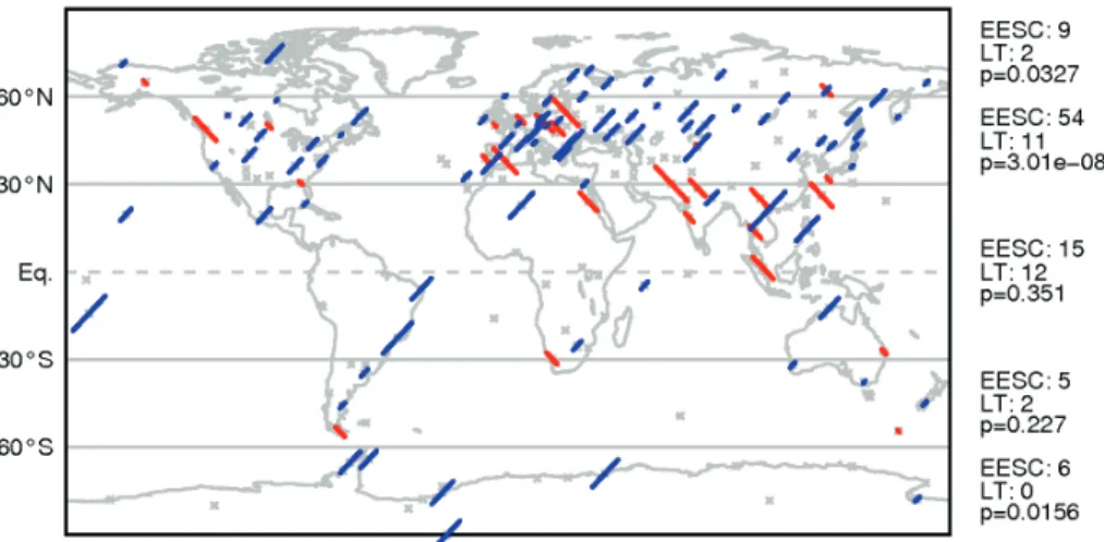
the stations in a given latitude belt showed a significant preference for one of two the models. The use of this test is justified because no spatial correlation was found (see Sect. 3.1). The two northern latitude belts show a clear preference for EESC to describe the measured ozone evolution (see Fig. 3). The results are significant at the 5% level (which corresponds to a 95% confidence interval) individually as well as 15
together. In the tropical latitude belt EESC and LT are nearly balanced. This result can be explained by the small trends compared to the high variation of total ozone. In the two southern latitude belts EESC is again preferred. The result of the southern mid-latitudes is not significant, probably because of the small number of stations, whereas both southern latitude belts together show a significant result. However, note that the 20
results of the South Polar latitudes should be ignored, since the amount of polar ozone depletion over Antarctica (ozone hole condition) is presently determined by dynamical factors, whereas ODS concentrations are still high enough not to be a limiting factor. In contrast, the situation in the Arctic is less dynamically driven (e.g., Solomon, 2007) and thus more strongly influenced by the present ODS levels which justifies including 25
the results for this region.
ACPD
10, 19005–19029, 2010Effectiveness of the Montreal Protocol to
protect the ozone layer
J. A. M ¨ader et al.
Title Page
Abstract Introduction
Conclusions References
Tables Figures
◭ ◮
◭ ◮
Back Close
Full Screen / Esc
Printer-friendly Version
Interactive Discussion
Discussion
P
a
per
|
Dis
cussion
P
a
per
|
Discussion
P
a
per
|
Discussio
n
P
a
per
|
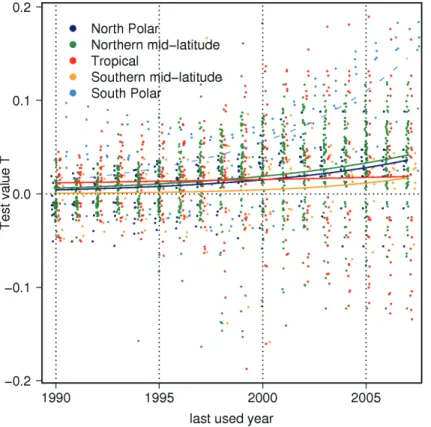
we repeated our analysis for different time windows. Figure 4 shows that the number of ozone series following EESC rather than LT increases with time, which supports the results.
In order to test the robustness of the results we performed a number of sensitivity studies (see Table 2). The last solar cycle which peaked in the year 2001 most likely 5
contributed to the observed ozone increase in the uppermost stratosphere since the mid 1990s and hence to the apparent turnaround in total ozone (Steinbrecht et al., 2004; Dameris et al., 2006). Based on our elimination process, solar flux, described by the solar flux intensity at 10.7 cm, is not one of the most important influence fac-tors for total ozone (M ¨ader et al., 2007). Consequently, inclusion of solar flux in the 10
equations does not affect our results significantly (see Table 2). In a recent study, Newman et al. (2007) postulated a new formulation to calculate EESC which includes an age-of-air dependent fractional release of ODS and an age-of-air spectrum. The replacement of the EESC time series used by WMO/UNEP (WMO, 2007) by two diff er-ent time series taken from Newman et al. (2007) does not change our results strongly 15
(see Table 2). (The two EESC variations were downloaded from the NASA Goddard website at http://code916.gsfc.nasa.gov/Data services/automailer/index.html. The fol-lowing parameters were used: WMO-Scenario: A1; Mean of age-of-air: 5.5 and 3.0 years; Width of Age-of-Air Spectrum: 1.5 years; Use Inorganic: yes; EESC withα: 60.) The robustness of the results was to be expected, since the different versions of EESC 20
are nearly identical up to linear transformations, and such alterations do not affect the significance of a variable in multiple linear regression.
4 Conclusions
In the late 1970s and the 1980s, i.e. since the paper of Molina and Rowland (1974), the search for a significant downward trend of total ozone measurements was an important 25
ACPD
10, 19005–19029, 2010Effectiveness of the Montreal Protocol to
protect the ozone layer
J. A. M ¨ader et al.
Title Page
Abstract Introduction
Conclusions References
Tables Figures
◭ ◮
◭ ◮
Back Close
Full Screen / Esc
Printer-friendly Version
Interactive Discussion
Discussion
P
a
per
|
Dis
cussion
P
a
per
|
Discussion
P
a
per
|
Discussio
n
P
a
per
|
explanatory variables of Quasi Biennial Oscillation and the eleven year solar cycle. Sig-nificant downward trends were first published in the Ozone Trend Panel report in 1989 (WMO, 1989) for northern mid-latitudes (where a large part of the population lives). This was viewed as evidence that the stratospheric ozone layer had been diminished by man made emissions of ODS. The Montreal Protocol (1987, including its enforce-5
ments in the subsequent years) has proved to be very effective to limit ODS emissions. More than twenty years later, the documentation of the beneficial effect of the Montreal protocol to protect the ozone layer is still not a simple task. One approach to this prob-lem has been the use of 2- and 3-dimensional numerical models to describe the effect of reductions of ODS on the ozone layer. However, because of the complex interactions 10
between transport and chemical processes (including e.g. heterogeneous processes on polar stratospheric clouds) and the limited computer resources such models need simplifications. Moreover, the validation against observations revealed largely varying degrees of success of the individual state-of-the-art models with respect to the repro-duction of individual processes including the observed ozone evolution (Eyring et al., 15
2007; WMO, 2007). Because of this large model spread the results concerning the effect of changes in man-made ODS emissions versus changes in dynamics remained controversial.
A complementary approach to describing the effect of changes in the column ozone is the use of statistical modelling. The results of such an approach, however, do not 20
provide direct causal relationship and only allow a sound interpretation if the used proxies are directly linked to the determining processes, which is generally difficult to prove. The proxies EL, T50 and PV470 identified by the elimination procedure, for example, are not readily attributable to a specific dynamical process but rather represent the combined effect of several processes including wave activity at different 25
ACPD
10, 19005–19029, 2010Effectiveness of the Montreal Protocol to
protect the ozone layer
J. A. M ¨ader et al.
Title Page
Abstract Introduction
Conclusions References
Tables Figures
◭ ◮
◭ ◮
Back Close
Full Screen / Esc
Printer-friendly Version
Interactive Discussion
Discussion
P
a
per
|
Dis
cussion
P
a
per
|
Discussion
P
a
per
|
Discussio
n
P
a
per
|
The aim of the study is not to provide reliable quantitative numbers concerning the attribution of ozone layer changes to chemical depletion or dynamics. The goal is rather to proof the effectiveness of the Montreal Protocol for the protection of the ozone layer. For this we compared two statistical ways to model the temporal evolution of the ozone layer, a linear upward trend (as a surrogate of the time evolution of the ozone layer 5
without a Montreal Protocol) and the temporal evolution attributable to the observed evolution of ODS following the Montreal protocol (EESC). We argue that the dynamical proxies, in particular EL, can represent dynamical changes in a sufficient way not to confuse the discrimination between a linear trend and an EESC trend. Note that our results have to be viewed as qualitative analysis. However, because of their robustness 10
we regard our results as clear and unprecedented evidence for the effectiveness of the Montreal Protocol for the protection of the ozone shield, proving the success of international cooperation between science, economy and politics.
Supplementary material related to this article is available online at: http://www.atmos-chem-phys-discuss.net/10/19005/2010/
15
acpd-10-19005-2010-supplement.pdf.
Acknowledgements. J. M. and D. B. were supported by the EU-projects CANDIDOZ and SCOUT-O3 within Framework Program 6 of the European Commission. H. R. was supported by the Competence Centre for the Environment and Sustainability (CCES) within the ETH-domain in Switzerland within the project EXTREMES: “Spatial extremes and environmental sustainabil-20
ity: Statistical methods and applications in geophysics and the environment”.
Data were provided by National Centers for Environmental Prediction (NCEP), European Cen-ter for Medium range Weather Forecasting (ECMWF), World Ozone and Ultraviolet Radiation Data Centre (WOUDC), National Aeronautics and Space Administration (NASA), British Antarc-tic Survey (BAS) and European Environment Agency (EEA).
ACPD
10, 19005–19029, 2010Effectiveness of the Montreal Protocol to
protect the ozone layer
J. A. M ¨ader et al.
Title Page
Abstract Introduction
Conclusions References
Tables Figures
◭ ◮
◭ ◮
Back Close
Full Screen / Esc
Printer-friendly Version
Interactive Discussion
Discussion
P
a
per
|
Dis
cussion
P
a
per
|
Discussion
P
a
per
|
Discussio
n
P
a
per
|
References
Appenzeller, C., Weiss, A. K., and Staehelin, J.: North Atlantic oscillation modulates total ozone winter trends, Geophys. Res. Lett., 27, 1131–1134, 2000.
Austin, J. and Wilson, R. J.: Ensemble simulations of the decline and recovery of stratospheric ozone, J. Geophys. Res.-Atmos., 111, D16314, doi:10.1029/2005jd006907, 2006.
5
Br ¨onnimann, S. and Hood, L. L.: Frequency of low-ozone events over Northwestern Europe in 1952–1963 and 1990–2000, Geophys. Res. Lett., 30, ASC8-1-5, doi:10.1029/2003gl018431, 2003.
Brunner, D., Staehelin, J., Maeder, J. A., Wohltmann, I., and Bodeker, G. E.: Variability and trends in total and vertically resolved stratospheric ozone based on the CATO ozone data 10
set, Atmos. Chem. Phys., 6, 4985–5008, doi:10.5194/acp-6-4985-2006, 2006.
Butchart, N., Scaife, A. A., Bourqui, M., de Grandpre, J., Hare, S. H. E., Kettleborough, J., Langematz, U., Manzini, E., Sassi, F., Shibata, K., Shindell, D., and Sigmond, M.: Simulations of antropogenic change in the strength of the Brewer-Dobson circulation, Clim. Dynam., 27, 727–741, doi:10.1007/s00382-006-0162-4, 2006.
15
Butchart, N. and Scaife, A. A.: Removal of chlorofluorocarbons by increased mass exchange between the stratosphere and troposphere in a changing climate, Nature, 410, 799–802, 2001.
Cressie, N. A. C.: Statistics for Spatial Data, revised edition, Wiley, New York, 1993.
Cressie, N. and Hawkins, D. M.: Robust estimation of the variogram, Int. Assoc. Math. Geol., 20
12, 115–125, 1980.
Dameris, M., Matthes, S., Deckert, R. Grewe, V., and Ponater, M.: Solar cycle effect delays on-set of ozone recovery, Geophys. Res. Lett., 33, L03806, doi:10.1029/2005GL02474, 2006. Engel, A., Strunk, M., Muller, M., Haase, H. P., Poss, C., Levin, I., and Schmidt, U.:
Tem-poral development of total chlorine in the high-latitude stratosphere based on reference 25
distributions of mean age derived from CO2 and SF6, J. Geophys. Res., 107(D12), 4136, doi:10.1029/2001JD000584, 2002.
Eyring, V., Waugh, D. W., Bodeker, G. E., Cordero, E., Akiyoshi, H., Austin, J. Beagley, S. R., Boville, B., Braesicke, P., Br ¨uhl, C., Butchart, N., Chipperfield, M. P., Dameris, M., Deck-ert, R., Deushi, M., Frith, S. M., Garcia, R. R., Gettelman, A., Giorgetta, M., Kinni-30
ACPD
10, 19005–19029, 2010Effectiveness of the Montreal Protocol to
protect the ozone layer
J. A. M ¨ader et al.
Title Page
Abstract Introduction
Conclusions References
Tables Figures
◭ ◮
◭ ◮
Back Close
Full Screen / Esc
Printer-friendly Version
Interactive Discussion
Discussion
P
a
per
|
Dis
cussion
P
a
per
|
Discussion
P
a
per
|
Discussio
n
P
a
per
|
Scinocca, J. F., Semeniuk, K., Shepherd, T. G., Shibata, K., Steil, B., Stolarski, R., Tian, W., and Yoshiki, M.: Multimodel projections of stratospheric ozone in the 21st century, J. Geo-phys. Res., 112, D16303, doi:10.1029/2006JD008332, 2007.
Farman, J. B., Gardiner, B. G., and Shanklin, J. D.: Large losses of total ozone in Antarctica reveal seasonal, Nature, 315, 207–210, 1985.
5
Fioletov, V. E., Labow, G., Evans, R., Hare, E. W., Kohler, U., McElroy, C. T., Miyagawa, K., Re-dondas, A., Savastiouk, V., Shalamyansky, A. M., Staehelin, J., Vanicek, K., and Weber, M.: Performance of ground-based total ozone network assessed using satellite data, J. Geophys. Res., 113, D14313, doi:10.1029/2008JD009809, 2008.
Guillas, S., Stein, M. L., Wuebbles, D. J., and Xia, J.: Using chemistry transport modeling in 10
statistical analysis of stratospheric ozone trends from observations, J. Geophys. Res., 109, D22303, doi:10.1029/2004JD005049, 2004.
Hadjinicolaou, P., Pyle, J., Chipperfield, M. P., and Kettleborough, J., Effect of interannual me-teorological variability on middle latitude O3, Geophys. Res. Lett., 24, 2993–2996, 1997. Hadjinicolaou, P., Jrrar, A., Pyle, J., and Bishop, L., The dynamically driven long-term trend in 15
stratospheric ozone over northern middle latitudes, Q. J. Roy. Meteorol. Soc., 128, 1393– 1412, 2002.
Harris, N. R. P., Kyr ¨o, E., Staehelin, J., Brunner, D., Andersen, S.-B., Godin-Beekmann, S., Dhomse, S., Hadjinicolaou, P., Hansen, G., Isaksen, I., Jrrar, A., Karpetchko, A., Kivi, R., Knudsen, B., Krizan, P., Lastovicka, J., Maeder, J., Orsolini, Y., Pyle, J. A., Rex, M., Vanicek, 20
K., Weber, M., Wohltmann, I., Zanis, P., and Zerefos, C.: Ozone trends at northern mid- and high latitudes – a European perspective, Ann. Geophys., 26, 1207–1220, doi:10.5194/angeo-26-1207-2008, 2008.
Hegglin, M. I. and Shepherd, T. G.: Large climate-induced changes in UV index and stratosphere-to-troposphere ozone flux, Nat. Geosci., 2, 687–691, 2009.
25
Hood, L. L. and Zaff, D. A.: Lower stratospheric stationary waves and the longitude dependence of ozone trends in winter, J. Geophys. Res.-Atmos., 100, 25791–25800, 1995.
Hood, L. L. and Soukharev, B. E.: Interannual variations of total ozone at northern midlatitudes correlated with stratospheric EP flux and potential vorticity, J. Atmos. Sci., 62, 3724–3740, 2005.
30
ACPD
10, 19005–19029, 2010Effectiveness of the Montreal Protocol to
protect the ozone layer
J. A. M ¨ader et al.
Title Page
Abstract Introduction
Conclusions References
Tables Figures
◭ ◮
◭ ◮
Back Close
Full Screen / Esc
Printer-friendly Version
Interactive Discussion
Discussion
P
a
per
|
Dis
cussion
P
a
per
|
Discussion
P
a
per
|
Discussio
n
P
a
per
|
Li, F., Stolarski, R. S., and Newman, P. A.: Stratospheric ozone in the post-CFC era, Atmos. Chem. Phys., 9, 2207–2213, doi:10.5194/acp-9-2207-2009, 2009.
M ¨ader, J. A., Staehelin, J., Brunner, D., Stahel, W. A., Wohltmann, I., and Peter, T.: Statistical modeling of total ozone: Selection of appropriate explanatory variables, J. Geophys. Res, 112, D11108, doi:10.1029/2006JD007694, 2007.
5
McLandress, C. and Shepherd, T. G.: Simulated anthropogenic changes in the Brewer-Dobson circulation, including its extension to higher latitudes, J. Clim., 22, 1516–1540, 2009. Molina, M. J. and Rowland, F. S.: Stratospheric sink for chlorofluoromethanes: chlorine
atom-catalysed destruction of ozone, Nature, 249, 810–812, 1974.
Montzka, S. A., Butler, J. H., Myers, R. C., Thompson, T. M., Swanson, T. H., Clarke, A. D., 10
Lock, L. T., and Elkins, J. W.: Decline in tropospheric abundance of halogen from halocar-bons: Implications for stratospheric ozone depletion, Science, 272, 1318–1322, 1996. Newchurch, M. J., Yang, E. S., Cunnold, D. M., Reinsel, G. C., Zawodny, J. M., and
Rus-sell, J. M.: Evidence for slowdown in stratospheric ozone loss: first stage of ozone recov-ery, J. Geophys. Res., 108, 4507, doi:10.1029/2003JD003471, 2003.
15
Newman, P. A., Daniel, J. S., Waugh, D. W., and Nash, E. R.: A new formulation of equivalent ef-fective stratospheric chlorine (EESC), Atmos. Chem. Phys., 7, 4537–4552, doi:10.5194/acp-7-4537-2007, 2007.
Newman, P. A., Nash, E. R., Kawa, S. R., Montzka, S. A., and Schauffler, S. M.: When will the Antarctic ozone hohle recover?, Geophys. Res. Lett., 33, L12814, 20
doi:10.1029/2005GL025232, 2006.
Orsolini, Y. and Doblas-Reyes, F.: Ozone signatures of climate patterns over the Euro-Atlantic sector in the spring, Q. J. Roy. Meteorol. Soc., 595, 3251–3263, 2003.
Percival, D. B., and Rothrock, D. A. : “Eyeballing” trends in climate time series: a coautionary note, J. Climate, 18, 886–891, 2005.
25
Peter, T.: Microphysics and heterogeneous chemistry of polar stratospheric clouds, Ann. Rev. Phys. Chem., 48, 785–822, 1997.
Randel, W., Wu, F., Russell, J., Waters, J., and Froidevaux, L.: Ozone and temperature-changes in the stratosphere following the eruption of Mount-Pinatubo, J. Geophys. Res, 100, 16753– 16764, 1995.
30
ACPD
10, 19005–19029, 2010Effectiveness of the Montreal Protocol to
protect the ozone layer
J. A. M ¨ader et al.
Title Page
Abstract Introduction
Conclusions References
Tables Figures
◭ ◮
◭ ◮
Back Close
Full Screen / Esc
Printer-friendly Version
Interactive Discussion
Discussion
P
a
per
|
Dis
cussion
P
a
per
|
Discussion
P
a
per
|
Discussio
n
P
a
per
|
Reinsel, G. C., Weatherhead, E. C., Tiao, G. C., Miller, A. J., Nagatani, R. M., Wuebbles, D. J., and Flynn, L. E.: On detection of turnaround and recovery in trend for ozone, J. Geophys. Res., 107, 4078, doi:10.1029/2001JD000500, 2002.
Rieder, H. E., Staehelin, J., Maeder, J. A., Peter, T., Ribatet, M., Davison, A. C., St ¨ubi, R., Weihs, P., and Holawe, F.: Extreme events in total ozone over Arosa – Part 2: Fingerprints of 5
atmospheric dynamics and chemistry and effects on mean values and long-term changes, Atmos. Chem. Phys. Discuss., 10, 12795–12826, doi:10.5194/acpd-10-12795-2010, 2010. Rinsland, C. P., Mahieu, E., Zander, R., Jones, N. B., Chipperfield, M. P., Goldman, A.,
Ander-son, J., Russell, J. M., III, Demoulin, P., Notholt, J., Toon, G. C., Blavier, J.-F., Sen, B., Suss-mann, R., Wood, S. W., Meier, A., Griffith, D. W. T., Chiou, L. S., Murcray F. J., Stephen, T. M., 10
Hase, F., Mikuteit, S., Schulz, A., and Blumenstock, T.: Long-term trends of inorganic chlorine from ground-based infrared solar spectra: past increases and evidence for stabilization, J. Geophys. Res., 108, 4252, doi:10.1029/2002JD003001, 2003.
Robock, A.: Volcanic eruptions and climate, Rev. Geophys., 38, 191–219, 2000.
Robock, A., Adams, T., Moore, M., Oman, L., and Stenchikov, G.: Southern Hemisphere at-15
mospheric circulation effects on th 1991 Mount Pinatubo Eruption, Geophys. Res. Lett., 34, L23710, doi:10.1029/2007GL031403, 2007.
Rosenfield, J. E., Considine, D. B., Meade, P. E., Bacmeister, J. T., Jackman, C. H., and Schoe-berl, M. R., Stratospheric effects of Mount Pinatubo aerosol studied with a coupled two-dimensional model, J. Geophys. Res., 102(D3), 3649–3670, 1997.
20
Shepherd, T. G.: Dynamics, stratospheric ozone, and climate change, Atmos.-Ocean, 46, 371– 392, 2008.
Solomon, S.: Stratospheric ozone depletion: a review of concepts and history, Rev. Geophys., 37, 275–316, 1999.
Solomon, S., Portmann, R. W., and Thompsom, D. W. J.: Contrasts between Antarctic and 25
arctic ozone depletion, P. Natl. Acad. Sci. USA, 104, 445–449, 2007.
Staehelin, J., Harris, N. R. P., Appenzeller, C., and Eberhard, J.: Ozone trends: A review, Rev. Geophys., 39, 231–290, 2001.
Staehelin, J., M ¨ader, J., Weiss, A. K., and Appenzeller, C.: Long-term ozone trends in Northern mid-latitudes with special emphasis on contribution of changes in dynamics, Phys. Chem. 30
Earth B, 27, 461–469, 2002.
ACPD
10, 19005–19029, 2010Effectiveness of the Montreal Protocol to
protect the ozone layer
J. A. M ¨ader et al.
Title Page
Abstract Introduction
Conclusions References
Tables Figures
◭ ◮
◭ ◮
Back Close
Full Screen / Esc
Printer-friendly Version
Interactive Discussion
Discussion
P
a
per
|
Dis
cussion
P
a
per
|
Discussion
P
a
per
|
Discussio
n
P
a
per
|
103(D15), 19183–19192, 1998.
Steinbrecht, W., Claude, H., and Winkler, P.: Enhanced upper stratospheric ozone: Sign of recovery or solar cycle effect?, J. Geophys. Res., 109, D02308, doi:10.1029/2003JD004284, 2004.
Stolarski, R. S. and Cicerone, R. J.: Stratospheric chlorine: a possible sink for ozone, Can. J. 5
Chem., 52, 1610–1615, 1974.
Thompson, D. W. J. and Wallace, J. M.: Annular modes in the extratropical circulation. Part I: Month-to-month variability, J. Climate, 13, 1000–1016, 2000.
Waugh, D. W., L. Oman, S. R. Kawa, R. S. Stolarski, S. Pawson, A. R. Douglass, P. A. Newman, and Nielsen, J. E.: Impacts of climate change on stratospheric ozone recovery, Geophys. 10
Res. Lett., 36(3), L03805, doi:10.1029/2008GL036223, 2009.
Weatherhead, C. and Anderson, S. B.: The search for signs of recovery of the ozone layer, Nature, 441, 39–45, doi:10.1038/nature04746, 2006.
Weatherhead, E. C., Reinsel, G. C., Tiao, G. C., Jackman, C. H., Bishop, L., Frith. S. M. H., DeLuisi. J., Keller, T., Oltmans, S. J., Fleming, E. L., Wuebbles, D. J., Kerr, J. B., Miller, A. J., 15
Herman, J., McPeters, R., Nagatani, R. M., and Frederick, J. E.: Detecting the recovery of total column ozone, J. Geophys. Res., 105, 22201–22210, 2000.
Wohltmann, I., Rex, M., Brunner, D., and M ¨ader, J.: Integreated equivalent latitude as a proxy for dynamical changes in ozone column, Geophys. Res. Lett., 32, L09811, doi:10.1029/2005GL022497, 2005.
20
World Meteorological Organisation, Report of the International Ozone Trends Panel 1988, Rep. 18, Global Ozone Research and Monitoring Project, Geneva, 1989.
World Meteorological Organisation. WMO Antarctic ozone bulletin 7, available at: http://www. wmo.ch/pages/prog/arep/gawozobull06 en.html, 2006.
World Meteorological Organisation. Scientific Assessment of Ozone Depletion: 2006, Rep. 50, 25
Global Ozone Research and Monitoring Project, Geneva, 2007.
Yang, E. S., Cunnold, D. M., Newchurch, M. J., and Salawitch, R. J.: Change in ozone trends at southern high latitudes, Geophys. Res. Lett., 32, L12812, doi:10.1029/2004GL02296, 2005. Yang, E.-S., Cunnold, D. M., Salawitch, R. J., McCormick, M. P., Russell III, J., Zawodny, J. M.,
Oltmans, S., and Newchurch, M. J.: Attribution of recovery in lower-stratospheric ozone, J. 30
ACPD
10, 19005–19029, 2010Effectiveness of the Montreal Protocol to
protect the ozone layer
J. A. M ¨ader et al.
Title Page
Abstract Introduction
Conclusions References
Tables Figures
◭ ◮
◭ ◮
Back Close
Full Screen / Esc
Printer-friendly Version
Interactive Discussion
Discussion
P
a
per
|
Dis
cussion
P
a
per
|
Discussion
P
a
per
|
Discussio
n
P
a
per
|
Table 1. Optimized versions of the regression model for total ozone (TOZ) of the five latitude
belts (see M ¨ader et al., 2007). The explanatory variables are sorted according to their rank determined in the model selection procedure. If not already included, a seasonal trend term (seas:Trend) was added for this study. The variableM (=month) represents the residual sea-sonal cycle; EL, the equivalent latitude proxy; Trend is either EESC or LT;TX, the temperature at pressure levelX;PV470, the potential vorticity at potential temperature level 470; SAD, the ver-tically integrated aerosol surface area density (describing the influence of volcanic eruptions);
VPSC, the cumulative volume of polar stratospheric clouds (describing polar ozone depletion); QBO30 the quasi biennial oscillation at pressure level 30 hPa. M is represented by 12 values. The notation seas:Trend indicates that different coefficients for Trend are estimated for each of the seasons (4 values). The other variables are characterized by a single (annual-mean) coefficient.
Latitude belt Optimized version of regression model
North Polar (NP): 11 stations north of 62◦
N
TOZ∼EL+M+seas : Trend+V
PSC+T50+SAD Northern Mid-latitude (NM):
65 stations 33◦
N–62◦
N
TOZ∼EL+M+T
10+seas : Trend+SAD
Tropical (TR): 27 stations 30◦
S–33◦
N
TOZ∼EL+M+seas : Trend
Southern Mid-latitude (SM): 7 stations 60◦
S–30◦
S
TOZ∼EL+T50+QBO30+M+seas : Trend
South Polar (SP): 6 stations south of 60◦
S
ACPD
10, 19005–19029, 2010Effectiveness of the Montreal Protocol to
protect the ozone layer
J. A. M ¨ader et al.
Title Page
Abstract Introduction
Conclusions References
Tables Figures
◭ ◮
◭ ◮
Back Close
Full Screen / Esc
Printer-friendly Version
Interactive Discussion
Discussion
P
a
per
|
Dis
cussion
P
a
per
|
Discussion
P
a
per
|
Discussio
n
P
a
per
|
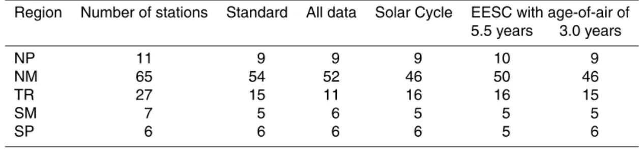
Table 2. Number of stations preferring EESC over LT in different versions of the basic model.
The column Standard corresponds to the main results of the paper. The column All data includes also the as “dubious” classified data from WOUDC (see Sect. 2). The fifth column refers to Sect. 3.2 on the influence of the solar cycle with solar flux at 10.7 cm as additional proxy. The last two columns represent the results if the new formulation for EESC by Newman et al. (2007) with an age-of-air of 5.5 and 3.0 years, respectively is used (see Sect. 3.2).
Region Number of stations Standard All data Solar Cycle EESC with age-of-air of 5.5 years 3.0 years
NP 11 9 9 9 10 9
NM 65 54 52 46 50 46
TR 27 15 11 16 16 15
SM 7 5 6 5 5 5
ACPD
10, 19005–19029, 2010Effectiveness of the Montreal Protocol to
protect the ozone layer
J. A. M ¨ader et al.
Title Page
Abstract Introduction
Conclusions References
Tables Figures
◭ ◮
◭ ◮
Back Close
Full Screen / Esc
Printer-friendly Version
Interactive Discussion
Discussion
P
a
per
|
Dis
cussion
P
a
per
|
Discussion
P
a
per
|
Discussio
n
P
a
per
|
Fig. 1. Left axis: Time series of Equivalent Effective Stratospheric Chlorine (EESC, provided
ACPD
10, 19005–19029, 2010Effectiveness of the Montreal Protocol to
protect the ozone layer
J. A. M ¨ader et al.
Title Page
Abstract Introduction
Conclusions References
Tables Figures
◭ ◮
◭ ◮
Back Close
Full Screen / Esc
Printer-friendly Version
Interactive Discussion
Discussion
P
a
per
|
Dis
cussion
P
a
per
|
Discussion
P
a
per
|
Discussio
n
P
a
per
|
Fig. 2. Spatial variograms for the (a) northern, (b) southern, (c) tropical latitude belts and
ACPD
10, 19005–19029, 2010Effectiveness of the Montreal Protocol to
protect the ozone layer
J. A. M ¨ader et al.
Title Page
Abstract Introduction
Conclusions References
Tables Figures
◭ ◮
◭ ◮
Back Close
Full Screen / Esc
Printer-friendly Version
Interactive Discussion
Discussion
P
a
per
|
Dis
cussion
P
a
per
|
Discussion
P
a
per
|
Discussio
n
P
a
per
|
Fig. 3.Map of ground based stations used in this study. Stations preferringEESCover linear
ACPD
10, 19005–19029, 2010Effectiveness of the Montreal Protocol to
protect the ozone layer
J. A. M ¨ader et al.
Title Page
Abstract Introduction
Conclusions References
Tables Figures
◭ ◮
◭ ◮
Back Close
Full Screen / Esc
Printer-friendly Version
Interactive Discussion
Discussion
P
a
per
|
Dis
cussion
P
a
per
|
Discussion
P
a
per
|
Discussio
n
P
a
per
|
Fig. 4.Evolution of the test valueT with increasing time window. Single points represent theT