Ground-based integrated path coherent differential absorption lidar measurement of CO<sub>2</sub>: hard target return

(1)

AMTD

5, 8579–8607, 2012

Hard target return

S. Ishii et al.

Title Page

Abstract Introduction

Conclusions References

Tables Figures

◭ ◮

Back Close

Full Screen / Esc

Printer-friendly Version Interactive Discussion

Discussion

P

a

per

|

Dis

cussion

P

a

per

|

Discussion

P

a

per

|

Discussio

n

P

a

per

|

Atmos. Meas. Tech. Discuss., 5, 8579–8607, 2012 www.atmos-meas-tech-discuss.net/5/8579/2012/ doi:10.5194/amtd-5-8579-2012

Atmospheric Measurement Techniques Discussions

This discussion paper is/has been under review for the journal Atmospheric Measurement Techniques (AMT). Please refer to the corresponding final paper in AMT if available.

Ground-based integrated path coherent

di

_ff

erential absorption lidar measurement

of CO

₂

: hard target return

S. Ishii1, M. Koyama2, P. Baron1, H. Iwai1, K. Mizutani1, T. Itabe1, A. Sato3, and K. Asai3

1

National Institute of Information and Communications Technology, 4-2-1 Nukuikitamachi, Kogenei, Tokyo 184-8795, Japan

2

Tokyo Metropolitan University, 6-6 Asahigaoka, Hino, Tokyo 191-0065, Japa 3

Tohoku Institute of Technology, 35-1 Yagiyamakasumi Taihaku, Sendai, Miyagi 982-8577, Japan

Received: 14 November 2012 – Accepted: 24 November 2012 – Published: 29 November 2012

Correspondence to: S. Ishii (sishii@nict.go.jp)

(2)

AMTD

5, 8579–8607, 2012

S. Ishii et al.

Title Page

Tables Figures

◭ ◮

Back Close

Full Screen / Esc

Discussion

P

a

per

|

Dis

cussion

P

a

per

|

Discussion

P

a

per

|

Discussio

n

P

a

per

|

Abstract

The National Institute of Information and Communications Technology (NICT) have made a great deal of effort to develop a coherent 2-µm differential absorption and wind lidar (Co2DiaWiL) for measuring CO₂and wind speed. First, coherent Integrated Path Differential Absorption (IPDA) lidar experiments were conducted using the Co2DiaWiL

5

and a hard target (surface return) located about 7.12 km south of NICT on 11, 27, and 28 December 2010. The detection sensitivity of a 2-µm IPDA lidar was examined in detail using the CO2 concentration measured by the hard target. The precisions of

CO2 measurement for the hard target and 900, 4500 and 27 000 shot pairs were 6.5,

2.8, and 1.2 %, respectively. The results indicated that a coherent IPDA lidar with a

10

laser operating at a high pulse repetition frequency of a few tens of KHz is necessary for measuring the CO2 concentration of the hard target with a precision of 1–2 ppm.

Statistical comparisons indicated that, although a small amount of in situ data and the fact that they were not co-located with the hard target made comparison di_fficult,

the CO2 volume mixing ratio measured with the Co2DiaWiL was about 5 ppm lower

15

than that measured with the in situ sensor. The statistical results indicated that there were no di_fferences between the hard target and atmospheric return measurements. A precision of 1.5 % was achieved from the atmospheric return, which is lower than that obtained from the hard-target returns. Although long-range DIfferential Absorption Lidar (DIAL) CO₂ measurement with the atmospheric return can result in highly

pre-20

cise measurement, the precision of the atmospheric return measurement was widely distributed comparing to that of the hard target return. Our results indicated that it is important to use a Q-switched laser to measure the range-gated di_fferential absorption optical depth with the atmospheric return and that it is better to simultaneously conduct both hard target and atmospheric return measurements to enable highly accurate CO2

25

measurement.

(3)

AMTD

5, 8579–8607, 2012

S. Ishii et al.

Title Page

Tables Figures

◭ ◮

Back Close

Full Screen / Esc

Discussion

P

a

per

|

Dis

cussion

P

a

per

|

Discussion

P

a

per

|

Discussio

n

P

a

per

|

1 Introduction

Atmospheric carbon dioxide (CO2) was roughly constant before the beginning of the

Industrial Revolution in the mid 18th century. Population growth has resulted in an in-crease in the consumption of fossil fuels, and human activities led to an inin-crease in CO2emission. Atmospheric CO2concentration has increased rapidly from 280 ppm to

5

greater than 380 ppm since the Industrial Revolution (IPCC, 2007). Data obtained from analyses of Antarctic ice cores and atmospheric observations indicate a relationship between the increase in CO2concentration and atmospheric temperature (Etheriddge

et al., 1996). Because of the presence of CO2sinks such as the oceans or terrestrial

ecosystems, atmospheric CO₂ increases at only half the rate of anthropogenic CO₂

10

emissions; however, in nature, the spatial-scale from regional to continental and the temporal variations in the CO2 sinks are not well understood due to limited

observa-tions (La Qu ´er ´e et al., 2009). Continuous monitoring of CO₂on a global scale is impor-tant for understanding the carbon cycle and estimating the carbon flux. Highly accurate ground-based and airborne measurements provide valuable data sets of the global

15

CO₂growth rate, seasonal information, hemispheric gradients, and so on. However, a lack of observation extends over a huge area. Ground-based and airborne measure-ments are not representative of the huge area to accurately infer carbon fluxes. Space-borne measurement is a promising approach for globally measuring the temporal and spatial distribution of XCO2(column-weighted dry-air mixing ratio of CO2). Spaceborne

20

XCO2measurement with a bias-free high precision of 1–2 ppm is necessary to improve

the carbon cycle. In 2009, the Greenhouse gas Observing SATellite (GOSAT) (Kuze et al., 2009), equipped with spaceborne passive sensors, was launched to continuously monitor the global total CO2column concentration. The Orbiting Carbon Observatory-2

(Crisp et al., 2004) and GOSAT-2 will be launched for the same purpose in the near

25

(4)

AMTD

5, 8579–8607, 2012

S. Ishii et al.

Title Page

Tables Figures

◭ ◮

Back Close

Full Screen / Esc

Discussion

P

a

per

|

Dis

cussion

P

a

per

|

Discussion

P

a

per

|

Discussio

n

P

a

per

|

An integrated path differential absorption (IPDA) lidar is one of the promising next-generation spaceborne sensors. The IPDA lidar uses a pulsed narrow-line width laser and a range-gated receiver. A Q-switched laser and range-gated receiver are helpful for distinguishing returns from the Earth’s surface from other returns such as aerosols and clouds. A di_fferential absorption lidar is not a_ffected by the presence of aerosols

5

and clouds, and it can be used in the day as well as at night at all latitudes, irrespective of season. The IPDA lidar has the potential of providing high measurement accuracy (bias close to zero), high precision (within a few ppm), ranging capability, and high sensitivity for detecting aerosol and clouds. The 1.6-µm and 2-µm spectral regions are suitable for XCO2measurement from space. The sensitivity of spaceborne lidar XCO2

10

measurement has been investigated (Menzies and Tratt, 2003; Ehret et al., 2008; Kawa et al., 2010). The NASA Langley Research Center (LaRC) and the Japan Aerospace Exploration Agency (JAXA) developed a 1.57-µm laser absorption spectrometer (LAS) with modulated continuous wave and direct detection (Browell et al., 2010; Sakaizawa et al., 2010). NASA Goddard Space Flight Center (Abshire et al., 2010) and Deutsches

15

Zentrum f ¨ur Luft-und Raumfahrt (German Aerospace Center) (Amediek et al., 2008) used a 1.57-µm pulse laser and direct detection. Simulated weighting functions of a

CO2 absorption cross-section (Menzies and Tratt, 2003; Ehret et al., 2008) shows

that, compared to the 1.57-µm spectral region, the 2.05-µm region is more sensitive to lower troposphere CO₂distribution where the sinks and sources interact with the

at-20

mosphere. Various 2-µm lasers have been developed for spaceborne IPDA lidar CO2

measurement (e.g. Yu et al., 2006; Sato et al., 2012). A 2.05-µm IPDA lidar is one of the most promising next-generation spaceborne sensors. The NASA Jet Propulsion Laboratory (JPL) (Spiers et al., 2011) is developing a 2.05-µm LAS with a contin-uous wave laser and heterodyne detection. NASA LaRC (Koch et al., 2004, 2008),

25

the Institute Pierre Simon Laplace ´Ecole Polytechnique (Gilbert et al., 2006, 2008), and the National Institute of Information and Communications Technology (NICT) (Ishii et al., 2010, 2012) reported 2.05-µm DIfferential Absorption Lidar (DIAL) by using a pulse laser, heterodyne detection, and aerosols and clouds (atmospheric return). We

(5)

AMTD

5, 8579–8607, 2012

S. Ishii et al.

Title Page

Tables Figures

◭ ◮

Back Close

Full Screen / Esc

Discussion

P

a

per

|

Dis

cussion

P

a

per

|

Discussion

P

a

per

|

Discussio

n

P

a

per

|

evaluated the performance of horizontal and vertical CO₂measurements using aerosol and cloud returns (Ishii et al., 2010, 2012). In this paper we describe the horizontal CO2

measurement using a hard target. In the next section, we briefly describe our coher-ent 2-µm differential absorption and wind lidar (Co2DiaWiL) and discuss the retrieval method of CO2and the error analysis in Sect. 3. We explain the measurement strategy

5

and experimental setup in Sect. 4. In Sect. 5, we describe the detection sensitivity of the IPDA lidar using experimental long-range CO₂measurements, the statistical results of

CO2measurements, and the comparison with the ground-based in situ measurements.

2 Coherent 2-µm differential absorption and wind lidar

The Co2DiaWiL specifications are listed in Table 1. Since the Co2DiaWiL is described

10

in detail in our previous work (Ishii et al., 2012), we present its main characteristics. The Co2DiaWiL has a single-frequency Q-switched Tm,Ho:YLF laser with laser fre-quency offset locking technique, a 10-cm-aperture Mersenne off-axis telescope, a two-axis scanning device, two heterodyne detectors, and signal processing devices. The single-frequency Q-switched Tm,Ho:YLF laser with a 2.05-µm operating wavelength

15

demonstrates 80-mJ output energy with a 150-ns pulse width (full width at half maxi-mum (FWHM)) at a 30-Hz pulse repetition frequency. The Co2DiaWiL uses two wave-lengths referred to as on- and off-line lasers for measuring CO2 concentration. The

two laser wavelengths are selected. The wavelength of the on-line laser corresponds to the center or wing of the absorption line of the target molecule, while the

wave-20

length of the off-line laser lies in the far wing of the absorption line. We use the R30 absorption line of the (20◦ 1)III←(00◦ 0) band of CO2. The wavelength of the on-line

laser can be set within the range of 2051.002–2051.058 nm using laser frequency o_ff -set locking. Based on the signal-to-noise ratio, we -set the wavelength of the on-line

laser at 2051.058 nm in order to conduct long-range CO2 measurements. The

wave-25

(6)

AMTD

5, 8579–8607, 2012

S. Ishii et al.

Title Page

Tables Figures

◭ ◮

Back Close

Full Screen / Esc

Discussion

P

a

per

|

Dis

cussion

P

a

per

|

Discussion

P

a

per

|

Discussio

n

P

a

per

|

transducer (PZT) that controls resonator length. The absolute frequency stability of the injected pulsed laser is 1 MHz at most. The o_ff-line laser is controlled only by adjusting the resonator temperature and piezoelectric movement of the output coupler element. The wavelength drift of the off-line laser is smaller than 7 pm, which corresponds to a maximum change of 0.04 % in the on-o_ffdi_fference absorption cross section. The

inter-5

ferences due to the presence of other atmospheric gases are almost negligible. The on-and off-line laser pulses are alternately switched every 1 shot. The pulsed laser beam is emitted into the atmosphere by using a 10-cm o_ff-axis telescope and a waterproof 2-axis scanning device. The signal backscattered by moving aerosol particles or re-flected by a hard target is detected using the heterodyne technique on an InGaAs-PIN

10

photodiode. The heterodyne detection is operated under shot-noise-limited condition of about 9 dB. A small portion of the pulsed laser beam is also detected using the het-erodyne technique to monitor the frequency of the outgoing laser pulse on a balanced InGaAs-PIN photodiode to monitor the frequency and lasing time of the outgoing laser. The outputs of these detectors are digitized at 500 MHz by using 8-bit analog-to-digital

15

(AD) converters. The power spectra of the outgoing on- and off-line laser pulses and backscattered signals were obtained by 4096- and 512-point fast Fourier transform (FFT), respectively. The power spectra of on- and off-line backscattered signals were obtained using an algorithm proposed by Frehlich et al. (1997). Data related to laser pulses with a frequency difference of more than 1.25 MHz from the average

interme-20

diate frequency (i.e. 105 MHz) were discarded. The ratio of discarded laser shot pairs was only around 5 % in the emitted laser shot pairs.

(7)

AMTD

5, 8579–8607, 2012

S. Ishii et al.

Title Page

Tables Figures

◭ ◮

Back Close

Full Screen / Esc

Discussion

P

a

per

|

Dis

cussion

P

a

per

|

Discussion

P

a

per

|

Discussio

n

P

a

per

|

3 Estimation of CO2and error analysis

The powerP_i₌On,Off(R) of backscattered signals from the hard target and atmosphere

can be expressed as

P_i(R)=ξi·P0,i·A·ρ

π·R2 ·exp(−2·

R Z

0

α_i(r) dr), (hard target) (1)

5

Pi(R)=

ξ_i·P0,i·A·β(R)

R2 ·exp(−2·

R Z

0

αi(r) dr), (atmosphere) (2)

whereR is the range,ξ_i is the total instrument efficiency for the wavelength i,P0,i is

the laser output power,Ais the receiver area,ρ is the surface reflectance, where we assume that the surface of the hard target is Lambertian, αi(r) is the extinction

co-efficient of the atmosphere, α_i(r) is defined as α_i (r)=αatm(r) +σi(r)ρCO₂Nair, where

10

σ_i(r) is the absorption cross section of CO2, ρCO₂ is the dry air volume mixing ratio

of CO₂,Nair is the dry air number density,αatm(r) is the extinction coefficient

associ-ated with any other extinction processes, andβ_i(R_j) is the backscattering coefficient of the atmosphere. Since the on- and off-line wavelengths are sufficiently close, we can neglect the wavelength dependence of instrument e_fficiency, surface reflectance, and

15

extinction coefficient except for CO2absorption.

The carrier-to-noise ratio CNR_i is defined as

CNR_i =hPi(R)i

P_i,N

, (3)

where

P_i,N

andhP_i(R)iare the mean power of the backscattered signal and the mean noise power. The theoretical signal-to-noise ratio SNR_i(R) for the squarer estimator

(8)

AMTD

5, 8579–8607, 2012

S. Ishii et al.

Title Page

Tables Figures

◭ ◮

Back Close

Full Screen / Esc

Discussion

P

a

per

|

Dis

cussion

P

a

per

|

Discussion

P

a

per

|

Discussio

n

P

a

per

|

described by Rye and Hardesty (1997) is given as

SNR_i(R)=

q

NL·NC·

CNR_i

1+CNR_i, (4)

whereNC is the number of coherent cells, and NL is the number of on- and off-line

laser shots. In this paper, NC for the atmospheric return signal is calculated using

Eq. (4) described by Gilbert et al. (2006), and for the hard target it is calculated using

5

Eq. (6.1–29) described by Goodman (2000).

By applying Eq. (1) to ranges R1 and R2, and to the on- and off-line wavelengths,

the di_fferential absorption optical depth (DAOD) due to CO₂ absorption in the range betweenR1andR2can be obtained as follows:

DAOD=

R₂

Z

R₁

ρCO₂(r)·Nair(r)· {σOn(r)−σOff(r)}dr=

1 2·log

_P

On(R1)·POff(R2)

POff(R1)·POn(R2)

. (5)

10

The CO2 volume mixing ratio is obtained by assuming that ρCO and meteorological

elements do not change betweenR1andR2.

ρCO₂=

1

2·Nair·σ·(R1−R2)

·DAOD−DAOD_H

2O

, (6)

Nair=

P k·T ·

1 1+ρH₂O

, (7)

15

whereσ (=σOn−σOff) is the difference between the absorption cross sections

corre-sponding to the wavelengths of the on- and off-line lasers,P is pressure,T is temper-ature,kis the Boltzmann constant,ρH₂O is the water vapor (H2O) volume mixing ratio,

and DAOD_H

2Ois the DAOD due to the H2O absorption betweenR1andR2.

(9)

AMTD

5, 8579–8607, 2012

S. Ishii et al.

Title Page

Tables Figures

◭ ◮

Back Close

Full Screen / Esc

Discussion

P

a

per

|

Dis

cussion

P

a

per

|

Discussion

P

a

per

|

Discussio

n

P

a

per

|

The relative error∆DAOD/DAOD between 0 andR is given by

∆DAOD (0,R) DAOD (0,R)

∼

= 1

2·DAOD(0,R)

s

1

SNR2_On(R)+ 1

SNR2_O_ff(R). (8)

The temporal cross correlation coefficient between POn(R) and POff(R) is required to

estimate the∆DAOD/DAOD. Although we assume the temporal cross correlation

coef-ficient as 0 to avoid the practical difficulties, the assumption does not affect the following

5

discussions. The relative error∆DAOD (R1,R2)/DAOD (R1,R2) betweenR1andR2can

be expressed as ∆DAOD (R1,R2)

DAOD (R1,R2)

∼

= 1

2·DAOD(R1,R2) s

1

SNR2_On(R1)

+ 1

SNR2_O_ff(R1)

+ 1

SNR2_On(R2)

+ 1

SNR2_O_ff(R2)

. (9)

The relative error∆ρCO₂/ρCO₂ is obtained using Eq. (10), DAOD, and meteorological

10

data as follows,

∆ρCO₂

ρCO₂ = s

∆NAir

NAir

2

+

∆σ σ

2

+

∆DAOD

DAOD

2

. (10)

To compare with the results of the hard target return, the CO2 volume mixing ratio

was also calculated using atmospheric returns and the slope method (Gilbert et al., 2006) under assumptions that the CO₂volume mixing ratio and CO₂ absorption cross

15

sections do not change betweenR1andR2.

4 Ground-based in situ measurements

(10)

AMTD

5, 8579–8607, 2012

S. Ishii et al.

Title Page

Tables Figures

◭ ◮

Back Close

Full Screen / Esc

Discussion

P

a

per

|

Dis

cussion

P

a

per

|

Discussion

P

a

per

|

Discussio

n

P

a

per

|

four-story building at NICT (a section of the building has five stories). The average val-ues of the meteorological data for each one-minute interval were automatically stored in a computer. The accuracies of pressure, temperature, and relative humidity wereare better than±0.5 hPa,±0.3◦C and±3 %, which lead to a total error of 0.1 % in the CO₂

volume mixing ratio on the DIAL measurement. Additional measurements of CO2and

5

H2O concentrations were carried out at one-minute intervals with an in situ sensor

(LI-COR Model LI-840, non-dispersive infrared CO₂/H₂O gas analyzer). The in situ sensor was installed in an observation room on the fifth-floor roof of the same building at NICT. Air entered the sensor at a flow rate of 1 L min−1through an inlet located approximately 2 m above the roof. The inlet for the in situ sensor was about 4 m higher than the

au-10

tomatic weather station. Calibrations were made before measurements with 0, 358,

and 452 ppm CO2 standard reference gases. The accuracy of the analyzer was

bet-ter than 1.5 %, and the root-mean-square value of the measured fluctuation was less than 1 ppm for a CO₂ volume mixing ratio of 370 ppm and for one-second filtering. In situ measurement was recorded after one-minute integration. The measured CO2data

15

were compared with the results obtained from DIAL measurement.

5 Experimental hard target measurement

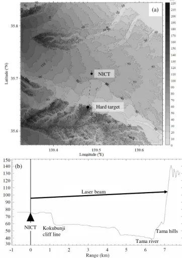
Figure 1a and b show the detailed topography and cross section around the target area. The laser beam was directed horizontally southward by using the 2-axis scan-ning device from NICT. It propagated 20 to 40 m above the surface and went through

20

a commercial area, highway, and the Tama river before it hit the hard target surface. The hard target is located approximately 7 km south of NICT. Figure 2a shows an ex-ample of the outgoing o_ff-line laser pulse signal (gray line) and the o_ff-line return signal (black line) obtained using 500-MHz-sampling-rate 8-bit AD converters. Arrows a and b indicate the peak time of lasing with Q-switching and the signal from the hard target.

25

Figure 2b and c show the square of the intermediate-frequency (IF) signals of the out-going off-line laser pulse and the off-line return signal. We define the range between the

(11)

AMTD

5, 8579–8607, 2012

S. Ishii et al.

Title Page

Tables Figures

◭ ◮

Back Close

Full Screen / Esc

Discussion

P

a

per

|

Dis

cussion

P

a

per

|

Discussion

P

a

per

|

Discussio

n

P

a

per

|

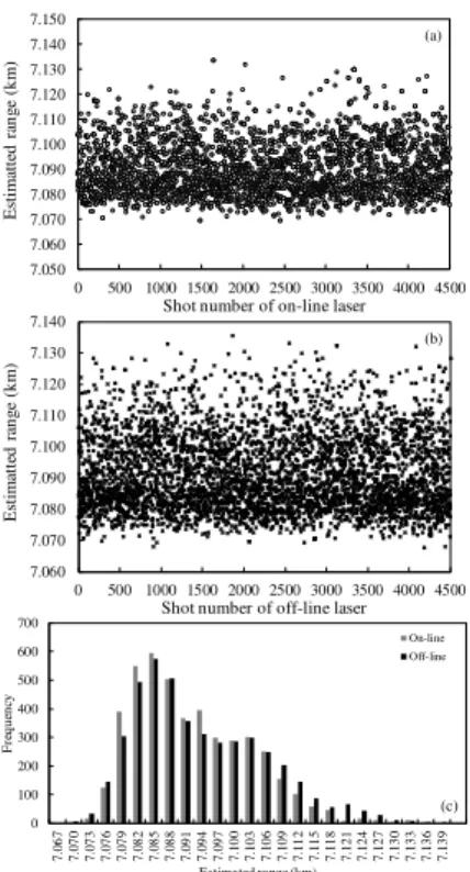
Co2DiaWiL and the hard target as the time difference at the two peaks. Figure 3a and b show examples of the range between the Co2DiaWiL and the hard target measured using the on- and off-line lasers from 01:50 to 01:55 JST on 11 December 2010. The range fluctuations shown in Figs. 3a through c were induced mainly by speckle-induced intensity fluctuation. We also believe that unstable pointing (e.g. swaying branches) of

5

the laser beam at the hard target might have caused range fluctuations. The aver-age ranges for the on- and off-line lasers for 1-min intervals were 7.089 (±0.010)– 7.091 (±0.011) and 7.091 (±0.012)–7.093 (±0.012) km, and the average ranges for 5-min interval were 7.090 (±0.011) and 7.092 (±0.012) km. The pulse width of 150 nsec corresponds to the range resolution of 0.023 km. Uncertainties of±0.012 km were

10

expected. The frequency distributions of the measured range for the on- and o_ff-line lasers were constructed for the on- and off-line lasers and are shown in Fig. 3c. This figure also shows that the measured range was distributed widely between 7.08 km and 7.11 km. We used the range resolution of 150 m to avoid speckle-induced intensity fluctuation for determining a correct range. The hard target was included at a range of

15

7.12 (±0.075) km.

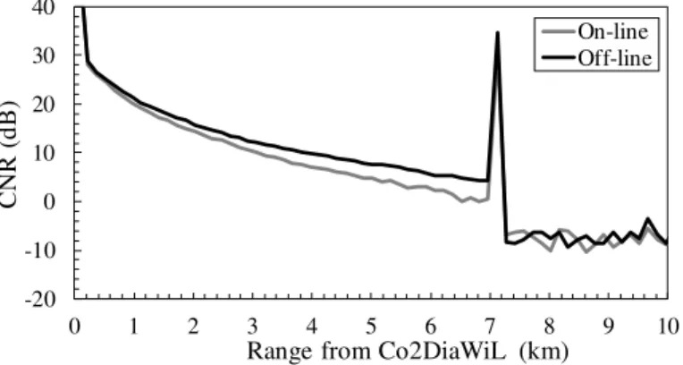
Figure 4 shows the CNR_i’s for the on-line (gray line) and o_ff-line (black line) laser pulses obtained from the hard target and atmospheric returns. The CNR_i was calcu-lated using the power spectra of the backscattered signals. The CNR_i’s of the on- and o_ff-line laser decreased slowly with increasing range up to 6.97 km, and a CNR_i higher

20

than 30 dB was observed at a range of 7.12 km. There are large differences more than 30 dB in the CNR at the ranges of 6.97 and 7.12 km. The hard target return was much stronger than the atmospheric return. Although the power of the atmospheric return could be included at the range of 7.12 km, the power was determined by the power of the hard target return signal.

25

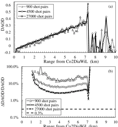
The relation between the range and DAOD (R1=0.974 km) for various shot pairs are

(12)

AMTD

5, 8579–8607, 2012

S. Ishii et al.

Title Page

Tables Figures

◭ ◮

Back Close

Full Screen / Esc

Discussion

P

a

per

|

Dis

cussion

P

a

per

|

Discussion

P

a

per

|

Discussio

n

P

a

per

|

fluctuations for distances greater than 4 km due to the decrease in the CNR_i, while for the 27 000 shot pairs, no large fluctuations were found. Figure 5b shows the relation between the range and relative error of the DAOD for the three shot pairs. The minimum relative errors of the DAOD for the three laser shot pairs in the range of 1 to 7 km were 13, 5.8, and 2.7 %, respectively. The relative error at short ranges was large due to the

5

small DAOD and low heterodyne efficiency. The heterodyne detection measurement

was also limited by speckle-induced noise. The relative error of the DAOD at the range of 7.12 km was about two times lower than the minimum relative errors due to the high CNR_i. The relative errors of the DAOD for the three laser shot pairs at the hard target bin were 6.5, 2.8, and 1.2 %, respectively.

10

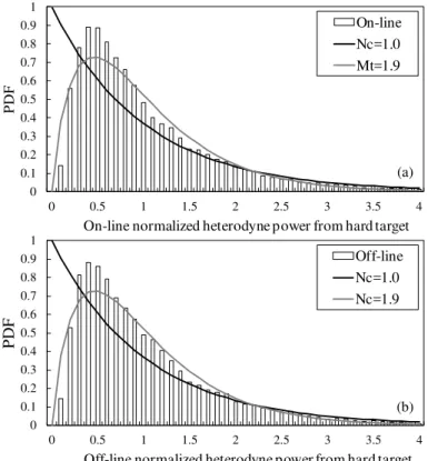
The probability density functions (PDFs) of on- and o_ff-line backscattered power

follows a gamma density function and NC is equal to the normalized variance of

the backscattered power, which is calculated using Eq. (6.1–29) described by Good-man (2000). The PDFs for on- and o_ff-line normalized power for the 27 000 shot pair measured from 01:50 to 02:20 JST on 11 December 2010 are shown in Fig. 6. The

15

PDF follows a gamma density function with NC=1.9 calculated using Eq. (6.1–29).

The calculated NC for the atmospheric return amounts to 6.7 using a pulse width of

150 ns and a range gate duration of 1000 ns. The calculated NC for the atmospheric

return is 3.5 times larger than theNC for the hard target return. Therefore, theNC for

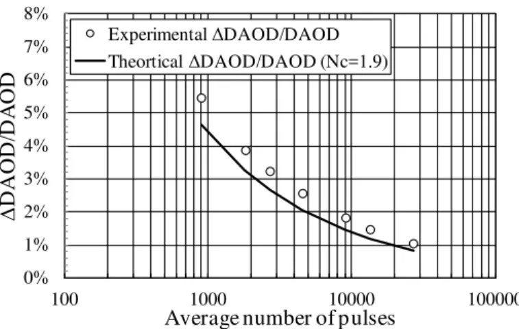
the hard target return is limited to improving the signal-to-noise ratio. Figure 7 shows

20

the relation between the average number of pulses and relative error of the DAOD for various shot pairs. We compared the theoretical and experimental values of the relative error of the DAOD. The theoretical values were calculated using Eqs. (4) and (9), and the results are shown as a black solid line in Fig. 7. The relative error of the DAOD by signal segmental averaging was found to decrease asN_L−1/2. To obtain a relative error

25

of 1–2 ppm under the assumptions that relative errors ofNair and σ were 0 %, our

re-sults indicate that the coherent IPDA lidar with the laser at a pulse repetition frequency of a few tens of KHz may be necessary to develop a coherent IPDA lidar.

(13)

AMTD

5, 8579–8607, 2012

S. Ishii et al.

Title Page

Tables Figures

◭ ◮

Back Close

Full Screen / Esc

Discussion

P

a

per

|

Dis

cussion

P

a

per

|

Discussion

P

a

per

|

Discussio

n

P

a

per

|

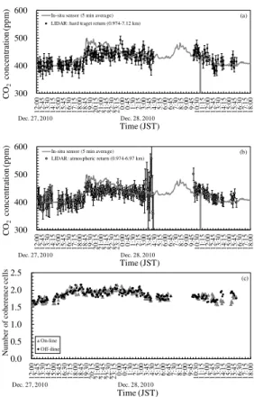
The horizontal experimental CO₂ measurements were done continuously from

12:10 JST on 27 December to 16:02 JST on 28 December 2010. The temporal vari-ations of the CO2volume mixing ratio measured using the Co2DiaWiL and the in situ

sensor are shown in Figs. 8a and b. The crosses and open circles show results ob-tained from hard target and atmospheric returns, respectively. The gray line shows

5

the data obtained from the in situ sensor. The time-series ofNC’s for on- and off-line

backscattered power is shown in Fig. 8c. The data show that the N_C’s for on- and off-line backscattered power were 1.5–1.9 during the day and 1.7-2.2 during at night. TheNC’s were roughly constant during the experimental period. The 4500 shot pairs

were used to estimate the CO₂ volume mixing ratios for both hard target and

atmo-10

spheric returns. The CO₂ volume mixing ratio for the hard target return was obtained

with a DAOD between 0.974 and 7.12 km and Eq. (5). The CO2 volume mixing ratio

for the atmospheric return was estimated for a column range from 0.974 to 6.97 km by using the slope method. There are 40 range-gated bins in the column range. The precision values of the Co2DiaWiL measurements for the hard target and atmospheric

15

returns shown in Figs. 8a and b were in the range of 2.8–5.3 and 1.5–11.0 %. Al-though meteorological data were not obtained close to the target surface, the data measured using our automatic weather station were used to calculate the absorption cross section of CO2 for the on- and off-line lasers. Since the difference between the

pressure measured using our automatic weather station and that at the hard target

20

was smaller than 1 hPa, the pressure induced error on the retrieved CO2volume

mix-ing ratio was negligible. However, if the temperature difference between the two points were larger than 1 K, it would result in a di_fference larger than 0.5 % in the CO₂ vol-ume mixing ratio. The error due to the difference between on- and off-line absorption

cross sections was 0.07 % in the CO2 volume mixing ratio on the Co2DiaWiL

mea-25

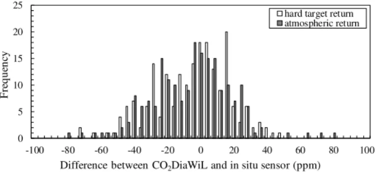
surement. The frequencies of di_fferences between the Co2DiaWiL measurements for

the hard target and atmospheric returns and the 5-min running averages of the in situ sensor are shown in Fig. 9. The CO2 volume mixing ratio estimated from the hard

(14)

AMTD

5, 8579–8607, 2012

S. Ishii et al.

Title Page

Tables Figures

◭ ◮

Back Close

Full Screen / Esc

Discussion

P

a

per

|

Dis

cussion

P

a

per

|

Discussion

P

a

per

|

Discussio

n

P

a

per

|

always lower/higher than the in situ sensor measurements. The average differences between the Co2DiaWiL measurements for the hard target and atmospheric returns were −4.6 and −5.0 ppm lower than the 5-min running averages of the in situ sen-sor. The difference of 5 ppm might be interpreted as a bias. The root-mean-square of the absolute values of difference between the Co2DiaWiL measurements for the hard

5

target and atmospheric returns and the 5-min running averages of the in situ sensor were 26.1 and 25.9 ppm. These statistical results indicate that the root-mean-square of the absolute values of the difference of the hard target return measurement was almost as the same as those of the atmospheric return measurement. The causes of the differences between the Co2DiaWiL and the in situ sensor are sampling volume,

10

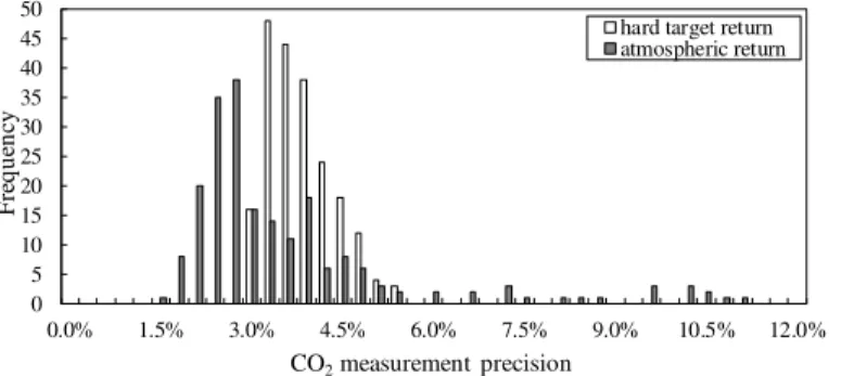
sampling location, and sampling height. It should also be emphasized that these re-sults were just an isolated comparison. Figure 10 shows the precision frequencies of the Co2DiaWiL measurements for the hard target and atmospheric returns conducted on 27 and 28 December. The precisions of the hard tarraget return measurement were mostly less than 3.8 %. On the other hand, the high precision frequencies of the

atmo-15

spheric return measurement were less than approximately 3.3 %. It should be noted that, although the long-range DIAL CO₂measurement with the atmospheric return can result in highly precise measurement, precision depends strongly on the fluctuation of the DAOD due to the decrease in the CNR. An important point is that the long-range

DIAL CO₂measurement with the hard target return measurement would be better for

20

maintaining data quality.

6 Conclusions

We used the Co2DiaWiL with a 2-µm single-frequency Q-switched laser with laser frequency offset locking to examine the detection sensitivity of a 2-µm IPDA lidar. Ex-perimental horizontal CO2measurements were conducted using hard target (surface)

25

and atmospheric (aerosol) returns in the western part of Tokyo on 11, 27 and 28 De-cember 2010. The CO2concentration was first measured with the 2-µm coherent IPDA

(15)

AMTD

5, 8579–8607, 2012

S. Ishii et al.

Title Page

Tables Figures

◭ ◮

Back Close

Full Screen / Esc

Discussion

P

a

per

|

Dis

cussion

P

a

per

|

Discussion

P

a

per

|

Discussio

n

P

a

per

|

lidar. The hard target is located about 7.12 km south of NICT. The results obtained from the hard target return were examined in detail and compared with those mea-sured from the atmospheric return and the in situ sensor. The range meamea-sured using the Co2DiaWiL showed a large fluctuation related mainly to speckle-induced intensity fluctuation. For coherent lidar, it is difficult to measure the range with a high precision of

5

less than 1 m due to the long laser pulse width. The precision of the range measured us-ing the Co2DiaWiL was within 0.012 km, which corresponded to the laser pulse width of 150 nsec. The precisions of CO2measurement due to the DAOD for the hard target and

900, 4500 and 27 000 shot pairs were 6.5, 2.8, and 1.2 %. The results indicated a laser operating at a high pulse repetition frequency of a few tens of KHz may be necessary

10

for the coherent IPDA lidar. Threfore, significant laser and optical device improvements

are necessary for future CO2 measurements with the coherent IPDA lidar. Although

the averages values of the differences between the Co2DiaWiL measurements were

about 5 ppm lower than the 5-min running averages of the in situ sensor, the compari-son between the Co2DiaWiL and in situ sensor CO2 measurements was difficult from

15

the point of the view of the one isolated comparison. Statistical comparisons indicated that there are no large di_fferences between hard target and atmospheric return mea-surements. The precision of the hard target return measurement was slightly worse than that of the atmospheric return measurement. TheNC for the hard target return

was limited to the improvement of the signal-to-noise ratio. The results indicate that

20

long-range DIAL CO2measurement with atmospheric return can enable highly precise

measurement. The precision of long-range DIAL CO2measurement with atmospheric

return depends strongly on the fluctuation of the DAOD. The long-range DIAL CO₂

measurement with hard target return may exhibit better data quality than that with at-mospheric return. The results presented in this paper indicate that it is important to use

25

a Q-switched laser to conduct range-resolved DAOD measurement with atmospheric return and that it is better to simultaneously conduct both hard target and atmospheric

(16)

AMTD

5, 8579–8607, 2012

S. Ishii et al.

Title Page

Tables Figures

◭ ◮

Back Close

Full Screen / Esc

Discussion

P

a

per

|

Dis

cussion

P

a

per

|

Discussion

P

a

per

|

Discussio

n

P

a

per

|

IPDA lidar with a Q-switched laser and a range-gated receiver has a great advantage in terms of discussing uncertainty due to the presence of aerosols and clouds.

References

Abshire, J. B., Riris, H., Allan, G. R., Weaver, C. J., Mao, J., Sun, X., Hasselbracj, W. E., Kawa, S. R., and Biraud, S.: Pulsed airborne lidar measurements of atmospheric CO₂column ab-5

sorption, Tellus, 62B, 770–783, 2010.

Amediek, A., Fix, A., Wirth, M., and Hert, G.: Development of an OPO system at 1.57 µm for integrated path DIAL measurement of atmospheric carbon dioxide, Appl. Phys., B92, 295– 302, 2008.

Browell, E. V., Dobler, J., Kooi, S. A., Choi, Y., Harrison, F. W., Moore III, B., and Zaccheo, T. 10

S.: Airborne validation of laser remote measurements of atmospheric carbon dioxide, Proc. 25th Int. Laser Radar Conf., 1, S6O–03, 2010.

Crisp, D., Atlas, R. M., Breon, F.-M., Brown, L. R., Burrows, J. P., Ciais, P., Connor, B. J., Doney, S. C., Fung, I. Y., Jacob, D. J., Miller, C. E., O’Brien, D., Pawson, S., Randerson, J. T., Rayner, P., Salawitch, R. J., Sander, S. P., Sen, B., Stephens, G. L., Tans, P. P., Toon, G. C., 15

Wennberg, P. O., Wofsy, S. C., Yung, Y. L., Kuang, Z., Chudasama, B., Sprague, G., Weiss, B., Pollock, R., Kenyon, D., and Schroll, S.: The Orbiting Carbon Observatory mission, Adv. Space. Res., 34, 700–709, 2004.

Ehret, G., Kiemle, C., Wirth, M., Amediek, A., Fix, A., and Houweling, S.: Space-borne remote sensing of CO₂, CH₄, and N₂O by integrated path differential absorption lidar: A sensitivity 20

analysis, Appl. Phys., B90, 593–608, 2008.

Etheridge, D. M., Steele, L. P., Langenfelds, R. L., Francey, R. J., Barnola, J.-M., and Morgan, V. I.: Natural and anthropogenic changes in atmospheric CO₂over the last 1000 years from air in Antarctic ice and firn, J. Geophys. Res., 101, 4115–4128, 1996.

Intergovernmental Panel on Climate Change (IPCC), Climate change 2007: The Physical Sci-25

ence Basis: Contribution of Working Group I to the Fourth Assessment Report of the In-tergovernmental Panel on Climate Change, edited by: Solomon, S., Qin, D., Manning, M., Chen, Z., Marquis, M., Averyt, K. B., Tignor, M., and Miller, H. L., Cambridge University Press, Cambridge, UK and New York, NY, USA, 996 pp., 2007.

(17)

AMTD

5, 8579–8607, 2012

S. Ishii et al.

Title Page

Tables Figures

◭ ◮

Back Close

Full Screen / Esc

Discussion

P

a

per

|

Dis

cussion

P

a

per

|

Discussion

P

a

per

|

Discussio

n

P

a

per

|

Gilbert, F., Flamant, P. H., Bruneau, D., and Loth, C.: Two-micrometer heterodyne differential absorption lidar measurements of the atmospheric CO₂ mixing ratio in the boundary layer, Appl. Opt., 45, 4448–4458, 2006.

Gilbert, F., Flamant, P. H., Cuesta, J., and Bruneau, D.: Vertical 2-µm heterodyne differential ab-sorption lidar measurements of mean CO₂mixing ratio in the troposphere. J. Atmos. Ocean. 5

Technol., 25, 1477–1499, 2008.

Goodman, J. W.: Statistical Optics, Wiley Classics Library, New York, 2000.

Ishii, S., Mizutani, K., Fukuoka, H., Ishikawa, T., Baron, P., Iwai, H., Aoki, T., Itabe, T., Sato, A., and Asai, K.: Coherent 2-µm differential absorption and wind lidar with conductively-cooled lLaser and two-axis scanning device, Appl. Opt., 49, 1809–1817, 2010.

10

Ishii, S., Mizutani, K., Baron, P., Iwai, H., Oda, R., Itabe, T., Fukuoka, H., Ishikawa, T., Koyama, M., Tanaka, T., Morino, I., Uchino, O., Sato, A., and Asai, K.: Partial CO₂Column-averaged Dry-air Mixing Ratio from Measurements by coherent 2-µm di_fferential absorption and wind lidar with Laser Frequency O_ffset Locking, J. Atmos. Ocea. Technol., 29, 1169–1181, doi.org/10.1175/JTECH-D-11-00180.1, 2012

15

Kawa, S. R., Mao, J., Abshire, J. B., Collatz, G. J., Sun, X., and Weaver, C. J.: Simulation studies for a space-based CO₂lidar mission, Tellus, 62B, 759–769, 2010.

Koch, G. J., Barnes, B. W., Petros, M., Beyon, J. Y., Amzajerdian, F., Yu, J., Davis, R. E., Ismail, S., Vay, S., Kavaya, M. J., and Singh, U. N.: Coherent differential absorption lidar measurements of CO₂, Appl. Opt., 43, 5092–5099, 2004.

20

Koch, G., Beyon, J. Y., Gilbert, F., Barnes, B. W., Ismail, S., Petros, M., Petzar, P. J., Yu, F. J., Modlin, E. A., Davis, K. J., and Singh, U. N.: Side-line tunable laser transmitter for differential absorption lidar measurements of CO₂: Design and application to atmospheric measure-ments, Appl. Opt., 47, 944–956, 2008.

Kuze, A., Suto, H., Nakajima, M., and Hamazaki, T.: Thermal and near infrared sensor for 25

carbon observation Fourier-transform spectrometer on the Greenhouse Gases Observing Satellite for greenhouse gases monitoring, Appl. Opt., 48, 6716–6733, 2009.

Le Qu ´er ´e, C., Raupach, M. R., Canadell, J. G., Marland, G., Marland, G., Bopp, L., Ciais, P., Conway, T. J., Doney, S. C., Feely, R. A., Foster, P., Friedlingstein, P., Gurney, K., Houghton, R. A., House, J. I., Huntingford, C., Levy, P. E., Lomas, M. R., Majkut, J., Metzl, N., Ometto, J. 30

(18)

AMTD

5, 8579–8607, 2012

S. Ishii et al.

Title Page

Tables Figures

◭ ◮

Back Close

Full Screen / Esc

Discussion

P

a

per

|

Dis

cussion

P

a

per

|

Discussion

P

a

per

|

Discussio

n

P

a

per

|

Menzies, R. T. and Tratt, D. M.: Differential laser absorption spectrometry for global profiling of tropospheric carbon dioxide: selection of optimum sounding frequencies for high-precision measurements, Appl. Opt., 42, 6569–6577, 2003.

Sakaizawa, D., Kawakami, S., Nakajima, M., Sawa, Y., and Matsueda, H.: Ground-based demonstration of CO₂remote sensor using 1.57 µm differential laser absorption spectrome-5

ter with direct detection, J. Appl. Remote. Sens., 4, 043548, doi:10.1117/1.3507092, 2010. Sato, A., Miyake, Y., Asai, K., Ishii, S., and Mizutani, K.: Tunable, Q-switched Tm,Ho:LLF laser

with a conductively cooled triangular prism rod, Appl. Opt., 51, 1236–1240, 2012.

Spiers, G. D., Menzies, R. T., Jacob, J., Christensen, L. E., Phillips, M. W., Choi, Y., and Browell, E. V.: Atmospheric CO₂measurements with a 2 µm airborne laser absorption spectrometer 10

employing coherent detection, Appl. Opt., 50, 2098–2111, 2011.

Yu, J., Trieu, B. C., Petros, M., Bai, Y., Petzar, P. J., Koch, G. J., Singh, U. N., and Kavaya, M. J.: Advanced 2-µm solid-state laser for wind and CO₂lidar applications, Society of Photo-Optical Instrumentation Engineers (SPIE) Conference Series, edited by: Singh, U. N., vol. 5575 of Society of Photo-Optical Instrumentation Engineers (SPIE) Conference Series, 6409, 15

C4091–C4091, doi:10.1117/12.696908, 2006.

(19)

AMTD

5, 8579–8607, 2012

S. Ishii et al.

Title Page

Tables Figures

◭ ◮

Back Close

Full Screen / Esc

Discussion

P

a

per

|

Dis

cussion

P

a

per

|

Discussion

P

a

per

|

Discussio

n

P

a

per

|

Table 1.Specifications of coherent 2-µm differential absorption and Doppler wind lidar. Transmitter

Laser Tm,Ho;YLF

Wavelength 2051.058 nm (On)/2051.250 nm (Off) Pulse energy 50-80 mJ/pulse (Operational)

Pulse width (FWHM) 150 ns

Pulse repetition 30 Hz

Polarization Circular

Receiver

Telescope type Mersenne off-axis

Diameter 0.1 m

Magnification 10

Detector for reference signal Balanced InGaAs-PIN photodiode Detector for backscattered signal InGaAs-PIN photodiode

Scanner

Scanning range Azimuth−10◦to 370◦ Elevation−20◦ to 200◦ E_ffective clear aperture 0.1 m

Scanning resolution 0.01◦

Scanning speed up to 60◦ s−1 Signal processing

Signal sampling frequency 500 MHz

Resolution 8 bits

FFT-point (reference) 4096

FFT-point (signal) 512

(20)

AMTD

5, 8579–8607, 2012

S. Ishii et al.

Title Page

Tables Figures

◭ ◮

Back Close

Full Screen / Esc

Discussion

P

a

per

|

Dis

cussion

P

a

per

|

Discussion

P

a

per

|

Discussio

n

P

a

per

|

Figure 1. (a) Map of area around NICT, hard target, and investigated areas. Contour lines a (a)

NICT

Hard target

(b)

Laser beam

NICT

Tama hills

Tama river Kokubunji

cliff line

Fig. 1. (a)Map of area around NICT, hard target, and investigated areas. Contour lines are represented at intervals of 10 m.(b)Cross section of topography data from NICT towards hard target.

(21)

AMTD

5, 8579–8607, 2012

S. Ishii et al.

Title Page Abstract Introduction Conclusions References Tables Figures ◭ ◮ ◭ ◮ Back Close

Full Screen / Esc

Printer-friendly Version Interactive Discussion Discussion P a per | Dis cussion P a per | Discussion P a per | Discussio n P a per | 0 500 1000 1500 2000 2500 3000 3500 4000

0 0.5 1 1.5 2 2.5 3 3.5 4 4.5 5

Re tu rn P o w er (a rb it ra ry u n it s)

Time after Q-switch triggering (µs) a (b) 0 50 100 150 200 250

0 5 10 15 20 25 30 35 40 45 50 55 60

IF s ig na l fr om A D c onve rt er

Time after Q-switch triggering (µs) Off-line signal Outgoing off-line laser

a (a) b 0 200 400 600 800 1000 1200 1400

0 5 10 15 20 25 30 35 40 45 50 55 60

Re tu rn P o w er (a rb it ra ry u n it s)

Time after Q-switch triggering (µs) b

(c)

(22)

AMTD

5, 8579–8607, 2012

S. Ishii et al.

Full Screen / Esc

Printer-friendly Version Interactive Discussion Discussion P a per | Dis cussion P a per | Discussion P a per | Discussio n P a per | 7.060 7.070 7.080 7.090 7.100 7.110 7.120 7.130 7.140

0 500 1000 1500 2000 2500 3000 3500 4000 4500

Es tim atte d r an g e ( k m )

Shot number of off-line laser 7.050 7.060 7.070 7.080 7.090 7.100 7.110 7.120 7.130 7.140 7.150

0 500 1000 1500 2000 2500 3000 3500 4000 4500

Es tim atte d r an g e ( k m )

Shot number of on-line laser (a) (b) 0 100 200 300 400 500 600 700 7. 06 7 7. 07 0 7. 07 3 7. 07 6 7. 07 9 7. 08 2 7. 08 5 7. 08 8 7. 09 1 7. 09 4 7. 09 7 7. 10 0 7. 10 3 7. 10 6 7. 10 9 7. 11 2 7. 11 5 7. 11 8 7. 12 1 7. 12 4 7. 12 7 7. 13 0 7. 13 3 7. 13 6 7. 13 9 F re que nc y

Estimated range (km)

On-line Off-line

(c)

Fig. 3.Range estimated from time difference between labels “a” and “b” in Fig. 2a for(a)on-line laser pulse and(b)off-line laser pulse and(c)frequency of estimated range for on- and offline laser pulse. Measurements were conducted from 01:50 to 01:55 JST on 11 December 2010.

(23)

AMTD

5, 8579–8607, 2012

S. Ishii et al.

Title Page

Tables Figures

◭ ◮

Back Close

Full Screen / Esc

Discussion

P

a

per

|

Dis

cussion

P

a

per

|

Discussion

P

a

per

|

Discussio

n

P

a

per

|

-20 -10 0 10 20 30 40

0 1 2 3 4 5 6 7 8 9 10

CN

R (d

B)

Range from Co2DiaWiL (km)

On-line Off-line

(24)

AMTD

5, 8579–8607, 2012

S. Ishii et al.

Title Page

Tables Figures

◭ ◮

Back Close

Full Screen / Esc

Discussion

P

a

per

|

Dis

cussion

P

a

per

|

Discussion

P

a

per

|

Discussio

n

P

a

per

|

-0.1 0 0.1 0.2 0.3 0.4 0.5 0.6

0 1 2 3 4 5 6 7 8 9 10

DAOD

900 shot pairs 4500 shot pairs 27000 shot pairs

(a)

0.1% 1.0% 10.0% 100.0%

0 1 2 3 4 5 6 7 8 9 10

∆

DAOD/

DAOD

900 shot pairs 4500 shot pairs 27000 shot pairs 0.3%

(b)

Fig. 5.Relation between range and(a)differential absorption optical depth (DAOD) and(b) rel-ative error of DAOD for 900 (open triangle), 4500 (open circle), and 27 000 (asterisk) shot pairs. Measurements were conducted from 01:50 to 02:20 JST on 11 December 2010. Dashed line shows relative error of DAOD of 0.3 % corresponding to 1 ppm in CO₂volume mixing ratio.

(25)

AMTD

5, 8579–8607, 2012

S. Ishii et al.

Title Page

Tables Figures

◭ ◮

Back Close

Full Screen / Esc

Discussion

P

a

per

|

Dis

cussion

P

a

per

|

Discussion

P

a

per

|

Discussio

n

P

a

per

|

0 0.1 0.2 0.3 0.4 0.5 0.6 0.7 0.8 0.9 1

0 0.5 1 1.5 2 2.5 3 3.5 4

P

DF

On-line normalized heterodyne power from hard target On-line Nc=1.0 Mt=1.9

(a)

0 0.1 0.2 0.3 0.4 0.5 0.6 0.7 0.8 0.9 1

0 0.5 1 1.5 2 2.5 3 3.5 4

P

DF

Off-line normalized heterodyne power from hard target Off-line Nc=1.0 Nc=1.9

(b)

(26)

AMTD

5, 8579–8607, 2012

S. Ishii et al.

Title Page

Tables Figures

◭ ◮

Back Close

Full Screen / Esc

Discussion

P

a

per

|

Dis

cussion

P

a

per

|

Discussion

P

a

per

|

Discussio

n

P

a

per

|

0% 1% 2% 3% 4% 5% 6% 7% 8%

100 1000 10000 100000

∆

DAOD/

DA

OD

Average number of pulses

Experimental ΔDAOD/DAOD Theortical ΔDAOD/DAOD (Nc=1.9)

Fig. 7.Calculated relative error of DAOD for various shot pairs. Measurements are same as those in Fig. 5.

(27)

AMTD

5, 8579–8607, 2012

S. Ishii et al.

Full Screen / Esc

Printer-friendly Version Interactive Discussion Discussion P a per | Dis cussion P a per | Discussion P a per | Discussio n P a per | ▲ ● 300 400 500 600 12 :00 12 :45 13 :30 14 :15 15 :00 15 :45 16 :30 17 :15 18 :00 18 :45 19 :30 20 :15 21 :00 21 :45 22 :30 23

:15 ₀:00 ₀:45 ₁:30 ₂:15 ₃:00 ₃:45 :30₄ ₅:15 ₆:00 ₆:45 ₇:30 ₈:15 ₉:00 ₉:45

10 :30 11 :15 12 :00 12 :45 13 :30 14 :15 15 :00 15 :45 16 :30 17 :15 18 :00 CO 2 con ce n tr at io n ( p p m ) Time (JST)

In-situ sensor (5 min average) LIDAR: hard traget return (0.974-7.12 km)

Dec. 27, 2010 Dec. 28, 2010

(a) 300 400 500 600 12 :00 12 :45 13 :30 14 :15 15 :00 15 :45 16 :30 17 :15 18 :00 18 :45 19 :30 20 :15 21 :00 21 :45 22 :30 23

:15 ₀:00 ₀:45 ₁:30 ₂:15 ₃:00 ₃:45 :30₄ ₅:15 ₆:00 ₆:45 ₇:30 ₈:15 ₉:00 ₉:45

10 :30 11 :15 12 :00 12 :45 13 :30 14 :15 15 :00 15 :45 16 :30 17 :15 18 :00 CO 2 con ce n tr at io n ( p p m ) Time (JST)

In-situ sensor (5 min average) LIDAR: atmospheric return (0.974-6.97 km)

Dec. 27, 2010 Dec. 28, 2010

(b) 0.0 0.5 1.0 1.5 2.0 2.5 12 :00 12 :45 13 :30 14 :15 15 :00 15 :45 16 :30 17 :15 18 :00 18 :45 19 :30 20 :15 21 :00 21 :45 22 :30 23

:15 ₀:00 ₀:45 ₁:30 ₂:15 ₃:00 ₃:45 :30₄ ₅:15 ₆:00 ₆:45 ₇:30 ₈:15 ₉:00 ₉:45

10 :30 11 :15 12 :00 12 :45 13 :30 14 :15 15 :00 15 :45 16 :30 17 :15 18 :00 N um be

r of c

ohe re nc e c e ll s Time (JST) On-line Off-iline

Dec. 27, 2010 Dec. 28, 2010

(c)

Fig. 8.Temporal variations of CO₂concentrations measured using Co2DiaWiL and in situ sen-sor on 27 and 28 December 2010: (a) hard target return and(b) atmospheric return. Laser frequency offset was 6.5 GHz for horizontal CO₂ measurement.(c) Time-series ofN_c: (•) on-and (

: (

▲

)

●

(28)

AMTD

5, 8579–8607, 2012

S. Ishii et al.

Title Page

Tables Figures

◭ ◮

Back Close

Full Screen / Esc

Discussion

P

a

per

|

Dis

cussion

P

a

per

|

Discussion

P

a

per

|

Discussio

n

P

a

per

|

0 5 10 15 20 25

-100 -80 -60 -40 -20 0 20 40 60 80 100

F

re

que

nc

y

Difference between CO2DiaWiL and in situ sensor (ppm) hard target return atmospheric return

Fig. 9.Frequency of differences between Co2DiaWiL measurements and 5-min running aver-ages of in situ sensor.

(29)

AMTD

5, 8579–8607, 2012

S. Ishii et al.

Title Page

Tables Figures

◭ ◮

Back Close

Full Screen / Esc

Discussion

P

a

per

|

Dis

cussion

P

a

per

|

Discussion

P

a

per

|

Discussio

n

P

a

per

|

Figure 10. Frequency of Co2DiaWiL measurement precision for hard target and atmospheric 0

5 10 15 20 25 30 35 40 45 50

0.0% 1.5% 3.0% 4.5% 6.0% 7.5% 9.0% 10.5% 12.0%

F

re

que

nc

y

CO2measurement precision

hard target return atmospheric return