www.atmos-meas-tech.net/9/5721/2016/ doi:10.5194/amt-9-5721-2016
© Author(s) 2016. CC Attribution 3.0 License.
2-D tomography of volcanic CO
2
from scanning hard-target
differential absorption lidar: the case of Solfatara,
Campi Flegrei (Italy)
Manuel Queißer1, Domenico Granieri2, and Mike Burton1
1School of Earth, Atmospheric and Environmental Sciences, University of Manchester, Oxford Road, Manchester M139PL, UK
2Istituto Nazionale di Geofisica e Vulcanologia (INGV), Sezione di Pisa, 50126 Pisa, Italy Correspondence to:Manuel Queißer (manuel.queisser@manchester.ac.uk)
Received: 16 May 2016 – Published in Atmos. Meas. Tech. Discuss.: 8 August 2016
Revised: 11 November 2016 – Accepted: 14 November 2016 – Published: 29 November 2016
Abstract. Solfatara is part of the active volcanic zone of Campi Flegrei (Italy), a densely populated urban area where ground uplift and increasing ground temperature are ob-served, connected with rising rates of CO2emission. A ma-jor pathway of CO2release at Campi Flegrei is diffuse soil degassing, and therefore quantifying diffuse CO2 emission rates is of vital interest. Conventional in situ probing of soil gas emissions with accumulation chambers is accurate over a small footprint but requires significant time and effort to cover large areas. An alternative approach is differential ab-sorption lidar, which allows for a fast and spatially integrated measurement. Here, a portable hard-target differential ab-sorption lidar has been used to acquire horizontal 1-D pro-files of column-integrated CO2 concentration at the Solfa-tara crater. To capture heterogenic features in the CO2 dis-tribution, a 2-D tomographic map of the CO2 distribution has been inverted from the 1-D profiles. The scan was per-formed one-sided, which is unfavorable for the inverse prob-lem. Nonetheless, the result is in agreement with independent measurements and furthermore confirms an area of anoma-lous CO2 degassing along the eastern edge as well as the center of the Solfatara crater. The method may have impor-tant implications for measurements of degassing features that can only be accessed from limited angles, such as airborne sensing of volcanic plumes. CO2 fluxes retrieved from the 2-D map are comparable, but modestly higher than emission rates from previous studies, perhaps reflecting an increase in CO2flux or a more integrated measurement or both.
1 Introduction
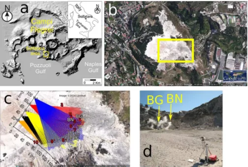
Figure 1.Geography and measurement geometry.(a)Location of the Solfatara crater as part of the volcanic area of Campi Flegrei, near Naples (Italy).(b)Nadir photo of Solfatara crater. The rectangle contains the region of interest.(c)Zoom of area outlined by the rectangle depicting the five instrument positions P1 to P5 with the following UTM coordinates: P1 (427476, 4519921), P2 (427485, 4519935), P3 (427495, 4519949), P4 (427507, 4519967) and P5 (427520, 4519986). Also shown are the respective range vectors (rays) for all five scans and the numbered locations of the LI-COR measurements.(d)Photo taken during the scan at P5 looking towards east. The largest clouds of condensed water aerosol appeared near the main vents (Bocca Nuova, BN, and Bocca Grande, BG) on the left. The CO2DIAL, visible in the
lower right corner, comprised of the tripod carrying the telescope (with transmitter unit) and the main unit (red box).
it may be dangerous to perform in situ measurements from within the volcanic plume (e.g., due to toxic gases or low visibility near the crater mouth). Secondly, in situ methods allow for a very accurate estimation of CO2 concentration, but only in the vicinity of the measurement point, potentially missing significant contributions from in between the mea-surement points.
Remote sensing techniques (see Platt et al., 2015, for overview of state of the art), notably active remote sensing platforms, including differential absorption lidar (DIAL) and spectrometers (Menzies and Chahine, 1974; Weibring et al., 1998; Koch et al., 2004; Kameyama et al., 2009), acquire columns of range-resolved (Sakaizawa et al., 2009; Aiuppa et al., 2015) or column-averaged (Amediek et al., 2008; Kameyama et al., 2009) CO2 concentrations. They provide a powerful tool to overcome the aforementioned drawbacks of in situ measurement techniques by offering a faster, safer and more comprehensive acquisition (spatial coverage yields inclusive CO2concentration profiles). Moreover, there is no need for receivers or retroreflectors at the opposite end of the measurement column, which not only increases flexibil-ity and timeliness of the acquisition but also is crucial for some measurements, including airborne or spaceborne acqui-sitions.
Active remote sensing platforms based on hard-target DIAL (topographic target DIAL) using continuous wave lasers can be made compact, rugged and portable, which
is desirable for platform-independent measurement of atmo-spheric CO2, be it ground based or airborne (Sakaizawa et al., 2013; Queißer et al., 2015a). However, the drawback compared with “traditional”, pulsed DIAL is that no range-resolved CO2concentrations are measured, but column den-sities (in m−2)or, as in this work, path length concentra-tion products are (called “path amount” hereafter, in ppm m). Hence, during a scanning measurement, no 2-D concentra-tion maps are obtained, but 1-D profiles of path amounts, that is, values of path amounts versus scanning angle. To obtain gas fluxes 1-D profiles suffice. However, there are good rea-sons to obtain gas distribution information (e.g., to localize flux hot spots), which is particularly important for heteroge-neous CO2emissions, including sites with both diffuse and vented degassing. It would be very desirable, and this was the motivation of this work, to use the 1-D profiles of path amounts to reconstruct a 2-D map that contains the geome-try of the anomalous CO2release, leaving aside precise CO2 mixing ratios. Note that tomographic reconstructions of vol-canic gas plumes have already been performed, however, for SO2and using passive remote sensing techniques (Kazahaya et al., 2008; Wright et al., 2008; Johansson et al., 2009).
Figure 2.Scheme of the CO2DIAL as used for this experiment. EOM: electro-optical modulator; DLEM: range finder module; EDFA:
erbium doped fiber amplifier. The beam pick is a glass wedge and reflects part of the transmitted light back into an integrating sphere (depicted as diffuser). ADC: analog-to-digital converter; DAC: digital-to-analog converter. The CO2cell is used to calibrate the seed laser
wavelengths. To minimize hard-target and turbulence-related speckle noise the collimator used had a relatively high divergence of 1.7 mrad, while the telescope field of view was 1.5 mrad. For mechanical reasons the optical band pass filter was mounted before the collimating lens. The change in transmission spectrum can be neglected.
resulting from two large collapses, the last one∼15 ka ago (Scarpati et al., 1993). CF is in direct vicinity to the metropo-lis of Naples and thus a direct threat to millions of residents. Thanks to its accessibility and strong CO2degassing Solfa-tara provides almost a model like volcano, a natural labo-ratory, to test new sensing approaches. However, it is part of one of the most dangerous volcanic zones in the world, show-ing ground uplift coupled with seismic activity with magma degassing likely having a significant role in triggering unrest (Chiodini at al., 2010). Solfatara therefore merits particular monitoring efforts and any new results on observables, may they stem from well-tried or new methods, are of direct im-portance to understand the fate of this active volcanic system.
2 Methods
2.1 Measuring 1-D profiles of CO2path amounts
The CO2DIAL (Fig. 2) is an active remote sensing platform based on the differential absorption lidar principle (Koch et al., 2004; Amediek et al., 2008). It is a further development of the portable instrument described in Queißer et al. (2015a, b). Specifics about the instrument and how CO2path amounts were retrieved are explained in detail in Queißer et al. (2016). Here, only a brief overview is given. By taking the ratio of the optical powers associated with the received signals for the wavelengths coinciding with an absorption line of CO2and the wavelength at the line edge,λONandλOFF, respectively,
one arrives at
2 R Z
0
dr1σ (r)NCO2(r)= −ln P (λ
ON) P (λOFF)ref P (λOFF) P (λON)ref
(1)
≡1τ, (2)
which is the differential optical depth1τ, the key quantity to be measured.NCO2is the CO2number densityRis the range, i.e., the distance between the instrument and the hard tar-get,1σ is the difference between the molecular absorption cross sections of CO2associated withλONandλOFF,P (λ)is the received (“science”) andP (λ)refis the transmitted opti-cal power (“reference”). The latter is measured as a reference to normalize fluctuations of the transmitted power. The nor-malized optical power in Eq. (1) is referred to as grand ratio (GR):
GR=P (λON) P (λOFF)ref P (λOFF) P (λON)ref
. (3)
and a maximum of 1.5 W. A glass wedge scatters a frac-tion of the transmitted light into an integrating sphere where the reference detector is mounted, which measuresP (λON) andP (λOFF). The transmitted light is diffusively backscat-tered by a hard target, which can be any surface located up to∼2000 m away from the instrument, and is received by a 200 mm diameter Schmidt–Cassegrain telescope with a focal length of 1950 mm and field of view of∼1.5 mrad. Typically the received optical power is a couple of nW at a bandwidth integrated noise of∼1 pW (root mean squared noise equiva-lent power). The analog-to-digital converter (ADC) operates at 250 kSamples s−1and has a resolution of 16 bit. The inte-gration time per scan angle was set to 4000 EOM modulation periods, which corresponds to data chunks of length 784 ms (integration time) for both science and reference channel. Each of these four chunks of data is demodulated using a digital lock-in routine following Dobler et al. (2013). After the lock-in operation one arrives at four DC signals, associ-ated with the optical powers P (λON),P (λOFF),P (λON)ref andP (λOFF)ref.1τ is calculated using the right-hand side of Eq. (1), after taking the mean of each of the four signals. However, to retrieve CO2path amounts the left-hand side of Eq. (1) was not used. Instead, to account for the instrumen-tal offset of1τ, prior to scanning the volcanic plume, values of 1τ were acquired for different R in the ambient atmo-sphere (Queißer et al., 2016). The points were used to fit a calibration curve. The ordinate atR=0 gave the instrumen-tal offset. The calibration curve was used to convert the mea-sured in-plume1τ to CO2path amountsYCO2 (in ppm m). Column-averaged CO2mixing ratiosXCO2,av(in ppm) were obtained by dividing path amounts by the hard-target range R. Note thatXCO2,av was mainly retrieved for display pur-poses rather than for data processing. The range was mea-sured by an onboard range finder (DLEM, Jenoptik, Ger-many), based on a 1550 nm lidar with pulse energy of 500 µJ and accuracy<1 m. By pivoting the receiver–transmitter unit using a step motor, values forYCO2per heading were attained and hence 1-D profiles.
The precision of the column-averaged CO2 mixing ratio was evaluated as
1X
CO2,av XCO2,av
2
=S/N−2+ σ
R hRi
2
+δSpeckle2 , (4) with the signal-to-noise-ratio (S/N) of
S/N= σGR
hGRi 1 ln(hGRi)
−1
, (5)
wherehGRiandσGRare the mean and standard deviation of the grand ratio, respectively. They were estimated from time series acquired at fixed angles in between the scans at CF. TheS/Naccounts for all noise sources occurring during ac-quisition, including instrumental noise, non-stationary base-line drift, solar background noise, atmospheric noise (mostly air turbulence) and perturbation by aerosol scattering (e.g.,
condensed water vapor). The second term depicts the relative range uncertainty (standard deviation of rangesσRover mean of rangeshRi), which is typically∼1 m. The relative uncer-tainty due to hard-target speckle was estimated as (MacKer-row et al., 1997)
δSpeckle=
1.22λOFFR
Dξ , (6)
whereDis the spot diameter on the hard target (in m) andξ is the dimension of the telescope field of view (in m) on the hard target. Typical values were 25 and 42 cm, respectively.
2.2 Reconstructing a 2-D map of CO2mixing ratios
The goal is to obtain CO2mixing ratios (XCO2, in ppm) at a given point (x,y). The region of interest (area bounding the scans) was divided into grid cells with length1x (inx di-rection) and1y(inydirection). Within a given grid cell the associated mixing ratio is uniform.XCO2 was inferred from the measuredYCO2 using an inverse technique following Pe-done et al. (2014a). The CO2path amount is associated with the product of a range segment and the (uniform) CO2 mix-ing ratioXCO2 along that range segment. For a given beam path and heading angle (hereafter also referred to as ray) and forpgrid cells traversed by the ray the corresponding gov-erning equation can be written as
p X
i=1
riXCO2,i=YCO2, (7)
whereri depicts the length of the ray segment in grid cell i
p P
i=1 ri =R
.XCO2,i is the (unknown) CO2mixing ratio within grid celli(in ppm). Including all rays, one arrives at a system of linear equations, which can be written as
Lc=a, (8)
whereLis am×nmatrix, called geometry matrix.ndepicts the number of model grid cells. The elements ofLare the length of allmpaths forngrid cells. For instance, the ele-mentlm=21,n=6depicts the length of ray 21 in grid cell num-ber 6. To be able to apply Eq. (7) to the measuredYCO2, the associated rays were mapped onto (x,y) coordinates using xj,k=rj,kcos1ϕj andyj,k=rj,ksin1ϕj.ϕj is the cumu-lative heading angle of thejth ray determined from the scan-ning angular velocity and the time interval between the rays retrieved from the time stamps of the data. For a given rayj, rj,k is thekth path length increment, such that
N P
k=1
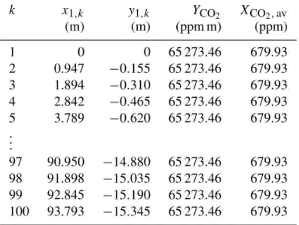
Table 1.Inversion data input file showing (x,y) coordinates with associated measuredYCO2andXCO2,av=YCO2/Rjof the first ray
(j=1) andxj=1,k,yj=1,kfor the first five and last four path length
increments.N=100.
k x1,k y1,k YCO2 XCO2,av
(m) (m) (ppm m) (ppm)
1 0 0 65 273.46 679.93
2 0.947 −0.155 65 273.46 679.93
3 1.894 −0.310 65 273.46 679.93
4 2.842 −0.465 65 273.46 679.93
5 3.789 −0.620 65 273.46 679.93
.. .
97 90.950 −14.880 65 273.46 679.93
98 91.898 −15.035 65 273.46 679.93
99 92.845 −15.190 65 273.46 679.93
100 93.793 −15.345 65 273.46 679.93
This was performed using the well-known rotation matrix with a rotation angle, which is the angle between the first ray and thex axis. TheYCO2 versus the resulting (x,y) co-ordinates formed the inversion input file (see Table 1 for an example). From the data in that input file an algorithm built the geometry matrix Lby using the (x,y) coordinates and computing the length of each ray in each model grid.cis a n×1 matrix containing uniform XCO2 per grid cell and is the desired quantity to be inverted.ais am×1 matrix con-taining the measured (observed)YCO2 for each ray, retrieved from the inversion input file. For simplicity,nx=ny, where nxandny are the number of grid cells inxandy direction, respectively. Thus,n=n2x.
Sincem > nthe system is overdetermined. This meansL
in Eq. (7) cannot be inverted to arrive atc, butchas to be approximated. This is done here using a least square fitting procedure. To solve Eq. (7) for ca least square solver, the MATLAB LSQR routine was used. The algorithm iteratively seeks values for c, which minimize the normalized misfit ka−Lck. Therefore,crepresents a model with a maximized likelihood of explaining the observed data a. By reshaping c into the measurement 2-D grid a 2-D map was obtained. Ordinary Kriging interpolation (Oliver, 1996) may then be applied to obtain a higher resolution estimate of the map.
2.3 CO2flux retrieval
From the inverted 2-D map ofXCO2the CO2flux (in kg s−1) was computed as
φCO2=10−6uNairMCO2 NA
Z Z
plume
dxdyXCO2,pl(x, y), (9)
whereXCO2,pl are the inverted, background-corrected CO2 mixing ratios computed as
XCO2,pl(x, y)=XCO2(x, y)−XCO2,bg, (10)
whereXCO2,bg=380 ppm is the background CO2mixing ra-tio at Solfatara measured in situ from an air sample, which was collected far from the degassing area, in accordance with Chiodini et al. (2011). The global average CO2level is now ∼400 ppm but this level may be quite different from one lo-cation to another for various reasons (latitude, weather condi-tions, seasonal effects, anthropogenic contributions). Inside and around the Solfatara there are many green areas (e.g., the nearby crater of Astroni), where the photosynthetic activity by plants likely causes the decrease in CO2levels compared to the more urbanized surroundings.uis the magnitude of the component of the plume transport speed perpendicular to the scanned cross section (in m s−1). Since the scans were performed along the horizontal planeurefers to the vertical component of the plume transport speed.Nairis the number density of air (in m−3), computed using meteorological data (pressure, temperature, humidity) acquired by a portable me-teorological station close to the instrument.MCO2 is the mo-lar mass of CO2 (in kg mol−1)andNA is Avogadro’s con-stant (in mol−1).
The plume transport speed was evaluated from digital video footage acquired during the measurement (Queißer et al., 2016), employing a video analysis program (Tracker from Open Source Physics). Condensed water vapor aerosol emitted by various vents in the region of interest was as-sumed to propagate with the same velocity as the volcanic CO2. At a given video frame a pixel was fixed and the calibrated propagated distance (in pixels) was measured as the video proceeded. Since the frame rate of the video was known (30 frames per second), the speed by which the tracked point and hence a parcel of gas was transported could be estimated.
The relative error of the CO2flux was estimated as 1φ
CO2 φCO2
2 =
1u
u 2
+ RR
plumedxdy1XCO2,pl(x, y) RR
plumedxdyXCO2,pl(x, y) !2
+ RR
plumedxdyσXCO2 RR
plumedxdyXCO2(x, y) !2
, (11) where1u is the absolute uncertainty of the plume speed, 1XCO2,plis the absolute error of the CO2mixing ratio (mea-surement precision) at a given point within the integrated area andσXCO2 is an estimate of the error of the inverted model. Figure 3 summarizes all main steps that were in-volved in the methods to retrieve the flux.
3 Results
Figure 3.Scheme summarizing the main data processing steps in-volved in this paper.
means of in situ measurements using a LI-COR CO2 ana-lyzer with 4 % accuracy. The LI-COR anaana-lyzer was measur-ing at the same height as the propagation height of the laser beam (ca. 2 m above ground). Due to logistical constraints the in situ measurements could only be measured the day before the experiment. Five scans were performed between 9:35 and 11:57 LT (duration 142 min) from five different lo-cations with a total ofm=627 beam paths (rays), which are shown along with the respective five instrument locations in Fig 1c. It is assumed that during the complete acquisition the CO2 distribution did not change (“frozen plume”). For each scan and for each heading differential optical depths1τ have been retrieved and converted intoYCO2 (andXCO2,av), as detailed in the method section. The resulting 1-D profiles of CO2 path amounts are shown in Fig. 3. Numerous wig-gles indicate widespread and heterogeneous degassing activ-ity, suggesting diffuse degassing or CO2advected by local wind eddies. In addition, there are symmetric features, such as around 26◦ in Fig. 3a, which appeared in scans carried
out prior to the experiment and the day before, thus suggest-ing vented degasssuggest-ing activity. The angular scannsuggest-ing veloc-ity was 2.1 mrad s−1, associated with an angular resolution of 1.65 mrad, which corresponds to a lateral resolution of around 24 cm between points in Fig. 3.
Before inverting XCO2, theYCO2 and the associated rays were mapped onto a (x, y) grid as detailed in the method section. The coordinate system was chosen such that the in-strument positions of all five scans were located on theyaxis
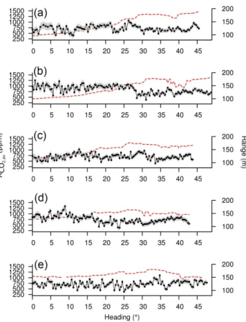
Figure 4.One-dimensional profiles ofXCO2,av, the total (not back-ground corrected) CO2mixing ratios, derived by dividing the path
amountsYCO2 (ppm m) per angle by the associated range. Each
value therefore represents a column-averaged mixing ratio. Each point corresponds to 784 ms integration time. For each profile and heading ranges are indicated by the red dashed line.(a) Profile acquired between 9:35:36 and 9:41:54. (b) Profile acquired be-tween 10:04:08 and 10:10:54.(c)Profile acquired between 10:31:24 and 10:37:28.(d)Profile acquired between 11:01:46 and 11:07:46.
(e)Profile acquired between 11:50:39 and 11:57:15. The grey enve-lope depicts precision (1 SD; Eq. 3).
(Fig. 1c). Table 1 shows an excerpt of the result of this proce-dure. Figure 5 shows the plot ofXCO2,avversusxj,kandyj,k (shown in Table 1). It represents a semi-quantitative map, in-dicating where high CO2concentrations are likely to be ex-pected and thus contains useful a priori information for the inversion.
capabil-ity to recover the true XCO2. Beyond that recovery became poorer. In addition, various inversions with random distri-bution of random XCO2 (drawn from a normal distribution with mean and standard deviations from the data presented in Fig. 5) were carried out that all yielded good recovery of XCO2. For the real data, however, already forn >16 the in-version yielded unreasonable high or low XCO2, which can be described as oscillatingXCO2. The difference between the synthetic and the real data vectorais that the former exhibits a higher variability of YCO2. This is illustrated in Fig. 7a, which shows the components ofa for one of the synthetic model realizations and the real data. The real data show high frequency components. One issue is the model discretization. In reality the scanned area was far from consisting of 16 grids with homogeneous XCO2 only, but instead was a complex distribution of an unknown number of CO2 patches, which leads to that spiky appearance of the real data vector. Further on, the more the “frozen” plume assumption holds the more the “humps” in Fig. 7a should resemble each other, since the x axis on Fig. 7a and b scales with the time of acquisition. For the synthetic case, there are five somewhat similar, but distorted, humps (Fig. 7b) due to the different viewing angle of each scan and differences in angle spans. This is, however, partially also the case for the real data vector (Fig. 7a), more so for the first four scans and less so for the last one. The spikes, i.e., the high frequency components, however, differ a lot, suggesting short-lived fluctuations on a small spatial scale that do not reappear between subsequent scans. This high frequency “noise” is due to the fact that actual fluctu-ations of theXCO2 occurred during the measurement. They happen on a faster timescale than the measurements of the five profiles (which took 142 min) and the scans themselves, violating our “frozen” plume assumption, at least for small patches of CO2. This leads to inconsistencies between the system of linear equations (there is no solution that satisfies all equations simultaneously) and hence problems to fit the spiky data.
Adding these high frequency components to the synthetic data by perturbing them using random perturbations drawn from normal distributedYCO2 (Fig. 7b) and performing versions gave an outcome very similar to the real data in-version. The inversion struggled to recover the true model XCO2 (Fig. 7c), yielding oscillations. To improve the real data inversion result synthetic inversions were performed af-ter smoothing the perturbed synthetic data vectora(Fig. 7b). Low-pass filtering the data, however, removes peaks and therefore falsifies the data, which the iteration then tries to fit, yielding poorly recovered XCO2. Smoothing had there-fore to be applied with care. As a result, moderately smooth-ing the data vectorausing a running average with window size 14 (rays) yielded reasonable recovery of the true model (Fig. 7d). However, performing synthetic tests with over 500 random arrangements of the grid cells occasionally led to oscillations in the model, meaning that the true XCO2 was over- and undershot again. It is important to note that this
Figure 5.Contour plot ofYCO2 after mapping them onto (x,y)
co-ordinates (which is the input to the inversion), divided by the range for all 627 beam paths (same as shown in Table 1 for first ray), which yields column-averaged mixing ratiosXCO2,av. Also shown
are the instrument positions (squares onyaxis) starting with P1 at
y=20 m. For display purposes the data have been regridded on a regular grid of 90×90 points using natural interpolation. One would expect high anomalous CO2mixing ratios near the main vents (BN and BG nearx=120 m,y=140 m) and the southern part of the area. Low anomalous CO2mixing ratios are to be expected in the
northwestern part. Note that due to the abundance of data some data points were masking each other. They were thus averaged, leading to a maximum mixing ratio lower than actually observed (e.g., in Fig. 4b).
occurred for grid cells at the model edges. This is the area where ray coverage is the poorest. It appeared that by in-creasing the number of grid cellsnthis issue worsened. The inverse problem is then still overdetermined in the sense of ray coverage (for instance, forn=64 on average there are still 10 rays per grid cell). However, this is not the case for the edge grid cells, as some grid cells are not traversed by some rays, which is aggravated with increasingn. Another contribution to the inconsistency of the system of linear equa-tions was given by rays that are not traversing the edge grid cells due to the topography of the hard target (slope). These two issues are illustrated in Fig. 7e. Moreover, albeit being a largely overdetermined (in fact mix-determined) problem, the rays are close to being parallel as the acquisition was one-sided and the instrument positions were not widely spread out. At best, the relatively large number of rays with similar angles provides redundancy of information. At worst, instead of adding extra information the lack of angle diversity may have contributed to the inconsistency of the problem, mak-ing the solution more unstable, meanmak-ing that a small change in data caused large variations in the model. Increasing the model grid numbernincreased inconsistency.
Figure 6.Synthetic inversion result withn=16 grid cells.(a)True model used to generate synthetic column-averagedYCO2. Each grid cell
is identified by a grid number. The dotted line outlines the ray coverage. The instrument positions are indicated.(b)Inverted model.(c)True and invertedXCO2versus grid cell. The invertedXCO2for grid 13 is off since the ray coverage associated with that area was poor.
of recovering an unknown and dynamic distribution of model parameters, in this caseXCO2, is inherently ill posed (Zhang et al., 2016), which implies non-uniqueness of the solution. This non-uniqueness is caused, for instance, by the unknown number of CO2patches or sources and their heterogenic and anisotropic distribution (Hamilton et al., 2014). In addition, a lack of observational data (mainly “frozen plume” assump-tion and angle diversity) caused inconsistency of the prob-lem, which led to both unrealistic model parameters (“os-cillations”) and a further amplified non-uniqueness of the model. It is apparent that increasing the grid number of the model would aggravate inconsistency and thus model error and non-uniqueness.
A more promising measure therefore was to omit parts of the rays, which is effectively smoothing the data vector without falsifying it, so that inconsistencies in Eq. (7) are reduced. Best results were obtained by selecting only every third ray and the corresponding YCO2 as input to the inver-sion.
As for the synthetic tests, a constantXCO2, the mean of the raw data (Fig. 5), was used as a starting model for inverting the real data. As a consequence of the discussion above the maximum feasible number of grid cells wasn=16 for a ro-bust inversion. The resulting grid length was1x=38 m and 1y=33 m. The inverted model is shown in Fig. 8a. To in-crease spatial resolution the inverted model was interpolated onto a grid with grid spacing 1x/8 and1y/8 using ordi-nary Kriging interpolation. The result is shown in Fig. 8b. The zones without ray coverage were excluded from the 2-D
map. Overlaying the resulting 2-D map of CO2mixing ratios with the map of Solfatara reveals a zone of increased anoma-lous CO2 degassing activity along the southeastern edge of Solfatara, which is in reasonable agreement with in situ data from the LI-COR CO2analyzer (Fig. 8c).
Figure 7.Synthetic inversion tests with perturbed data.(a)Data vectora(Eq. 7), showing the real and synthetic data (used for inversion
result in Fig. 6) versus ray number.(b)Synthetic data vector, perturbed synthetic data vector and smoothed perturbed synthetic data vector.
(c)Inversion result using the perturbed synthetic data from(b).(d)Inversion result using the smoothed perturbed synthetic data. As the true model values were drawn from a random distribution, the model arrangement differs between(c)and(d).(e)Scheme of a single grid cell at the model edge facing the instrument position with two subsequent rays that have traversed the same grid cells before reaching the displayed grid. As they are in the same grid and nearly parallel, Eq. (6) should yield almost identical path amounts for both rays. However, this is not the case since, due to the topography, their lengths differ. This adds inconsistency to Eq. (7). If as a remedy the number of model grid cells would be increased, for instance such that the grid spacing is halved (dotted lines), this would lead to grid cells without ray coverage, as illustrated here, and hence erroneous model values.
4 Discussion
Retrieving CO2 path amounts using calibration based on mixing ratios as done here is not optimal as the mixing ra-tios depend on temperature, pressure and humidity of the air. It was a solution that was adopted for practical reasons. Com-pared with the precision of the instrument the resulting bias was, however, low and could be neglected. Typically, the air temperature varied between 11 and 15◦C and relative hu-midity varied between 55 and 65 %. The air pressure was steady around 974 hPa. In a simplified estimation, this cor-responds to a bias of ∼1.5 % of the total column-averaged mixing ratio, which would correspond to around 9 ppm, as-suming typical measured path amounts and ranges. To put this into context, the error of the column-averaged mixing ra-tio was typically∼110 ppm (Fig. 3) and is dominated by the instrumentS/N. The associated increase in flux uncertainty would be less than 1 %. In the future, however, a better re-trieval scheme will be adopted. This is important as we strive to increase in the measurement precision of the CO2DIAL
to sense more subtle CO2emissions than at Solfatara and a bias related to uncertainty of the number density becomes relevant. Note that a bias of 20 ppm due to uncertainties in background mixing ratio would also entail a small decrease in measurement precision by∼4 % and an increase in flux error by roughly 2 %.
Figure 8.Retrieved 2-D model ofXCO2.(a)Inverted model ofXCO2.(b)InvertedXCO2 after ordinary Kriging interpolation (interpolated
grid size is 3.75 by 4.38 m). The ray coverage is depicted by the dotted line. The straight lines outline the grid.(c)XCO2superposed onto nadir
photo of Solfatara for those areas covered by the rays. To project the inverted model onto the map the function “overlay image” of Google Earth software has been used using altitude 0 relative to instrument altitude above ground. Also shown areXCO2from in situ measurements
(measurement points 3 to 10) using the LI-COR CO2analyzer. Note that the in situ values had been acquired a day before the scans and thus serve as an approximate reference only. Moreover, since measured column-integrated mixing ratios were below 1500 ppm, there is noXCO2
of 1500 ppm expected in the inversion result.
near 26◦in the first scan in Fig. 3a. The second scan (Fig. 3b) indicates a rather abrupt decrease inXCO2,av at 28◦, in line with the edge of the zone of elevated CO2 mixing ratios at the crater center (left part of Fig. 8c). This central degassing feature is coherent with results of recent campaigns (Granieri et al., 2010; Tassi et al., 2013; Bagnato et al., 2014). The in-crease in XCO2,av near 9◦ in Fig. 3d matches the position of the local peak in XCO2 between in situ points 7 and 8 in Fig. 6c. Provided sufficient rays, which was the case for the zones away from the edges of the 2-D map, disagreement be-tween the peaks in the 1-D data (Fig. 3) and those in the 2-D map (Fig. 6) are likely due to physical fluctuations in CO2 concentration (“frozen” plume approximation), as evinced in the result section. During acquisition one could visually iden-tify at least five small vents emitting water vapor and there-fore most likely also CO2. Though not recovered due to the limited spatial and temporal resolution of the inversion, this
advocates that there are in fact separate vents south of the main vents, near the edge of the Solfatara crater.
RetrievedXCO2 peak near 1300 ppm (2 m above ground), in line with the in situ LI-COR data, although not spatially matching them in places. This can be explained by the fact that the in situ values were acquired the day before so that local wind and thus dispersion patterns were different. Nev-ertheless, both the LI-COR in situ data and the inversion re-sult indicate high XCO2 near the main vents and along the crater edge. Near the main vents the highest CO2 mixing ratios in the 2-D map are located ca. 17 m west of BN. In fact, the whole zone of highXCO2 is shifted∼17 m north-west from where one would expect it. Since the predomi-nant wind direction at the time of acquisition was around 300◦, to first order one would expect the CO2 to disperse rather towards southeast, along the crater edge. The main vent area was at the edge of the scanned area. Note that the relative inversion residualka−Lck
average 18 % of 1XCO2,pl is unexplained by the model in Fig. 8a. Note that due to the non-uniqueness of the prob-lem a lower misfit does not imply that the inverted model is closer to the “true” model. For instance, increasing the grid number decreased the misfit but yielded models withXCO2 much larger than the maximum or lower than the minimum in Fig. 4. Although being close to the expected distribution, the mismatch is therefore likely due to a non-unique realization of the model. The latter is related to poor ray coverage for grid 16 (northeastern most), which is partly corresponding to the zone containing the main vents, and the error resulting from the low model discretization (in realityXCO2 was cer-tainly not constant over 30 m). Note that the acquisition fo-cused on the zone south of the main vents. Possibly, but less likely, CO2was advected slightly towards west due to disper-sive mechanism related to local wind eddies decoupled from the main wind direction. These dispersive mechanisms take place in any case and make a distinction between CO2from the main vents and the surrounding diffuse degassing chal-lenging. For that reason, in future acquisitions at that site the region of interest shall be scanned from instrument positions aligned along a half circle around the zone rather than using a “flat” scan geometry as chosen here.
For a comparison, CO2 fluxes were computed directly from the 1-D profiles (Fig. 4), that is, similar to Eq. (8) but using path amounts, ignoring any heterogeneity in the CO2 distribution. Given the uncertainty, the average flux of all five scans (1055±389 tons day−1) is compatible with the result obtained from the 2-D map (1465±798 tons day−1).
However, both the CO2 flux from the 2-D map and from the 1-D profiles are higher than fluxes previously es-timated. Pedone et al. (2014a) report a CO2 flux of only ∼300 tons day−1 in early 2013, but it focused on the area around the Solfatara main vents, that is, 8000 m2. In this study the area considered for flux computation was over 21 000 m2. Moreover, the average degassing rate at Solfa-tara has been increasing by ∼9 % each year over the past 10 years or so (Chiodini et al., 2010; d’Auria, 2015). The magnitude of the retrieved flux of this work equals the total CO2flux of diffuse degassing structure (which encompasses the Solfatara crater, the Pisciarelli fumaroles and the area around Solfatara crater) reported by Granieri et al. (2003), however, 13 years prior to this study, when emission rates were 1.0913 (or 3) times lower. A very rough extrapola-tion of the 1465 tons day−1 obtained here to the whole of Solfatara crater, that is, by assuming a constant flux per unit area (Queißer et al., 2016), would yield a flux between 2400 and 4700 tons day−1. This makes 1465 tons day−1 a coherent figure. Extrapolating the flux for the main vent area of 300 tons day−1 from 2013 would yield a flux of 390 tons day−1 in early 2016. Integrating CO2 mixing ra-tios of the area around the main vents only (bounded to the south by in situ point 6; Fig. 8c) yields a flux of 364± 206 tons day−1of CO2, in excellent agreement with the ex-trapolated flux. Finally, we note that to our knowledge all
former studies except one (Pedone et al., 2014a) inferred XCO2 and hence CO2 fluxes from a grid of point measure-ments. If the area associated with lower CO2 concentration was larger than the area with very high CO2concentration, point sampling may have missed degassing activity in be-tween the measurement points and so tended to yield lower flux values.
5 Conclusions
As magmatic CO2degassing rates are tracers for the dynam-ics and chemistry of the magma plumbing system beneath Campi Flegrei and at volcanic areas in general, a compre-hensive quantification of magmatic CO2degassing strength is of interest for volcanology and of vital importance for civil protection.
Scanning hard-target DIAL measurements has been per-formed at Solfatara crater (Campi Flegrei, Italy), which al-lowed an inclusive measurement of CO2amounts in the form of 1-D profiles of CO2 path amounts. From the 1-D pro-files a 2-D map of CO2mixing ratiosXCO2 has been recon-structed, outlining the main CO2distribution. Primarily the one-sided acquisition geometry of the input 1-D profiles and assumptions about the emission dynamics (“frozen” plume) increased inconsistency of the inverse problem and limited the feasible spatial resolution of the model.
However, the resulting map of XCO2 was in satisfactory agreement with independent measurements of CO2 mixing ratio. Therefore, the 2-D map was deemed to be useful to re-trieve the CO2 flux. The fluxes retrieved using that map is compatible with previous results. The 1-D profiles have been acquired from a single half space (one-sided), which indi-cates this tomography method to be potentially beneficial for scanning strongly non-isotropic CO2 distributions, such as diffuse emissions, that can be viewed from limited angles only, sites difficult to access (e.g., volcanic craters), or air-borne acquisitions. The authors expect a more adapted acqui-sition geometry to enhance resolution of the 2-D map, which would allow a more accurate gas flux estimation. However, more tests are necessary to assess general applicability and increase confidence in this method.
6 Data availability
The data as well as the MATLAB script used for the to-mographic inversion are available upon request from the Research Data Repository of the University of Manchester (UK).
Acknowledgements. The research leading to these results has received funding from the European Research Council under the European Union’s Seventh Framework Programme (FP/2007-2013)/ERC grant agreement no. 279802. Our gratitude goes to Rosario Avino and Antonio Carandente (INGV Osservatorio Vesuviano), who sampled the in situ CO2mixing ratios. We thank
Graham Allen (NASA Goddard Space Flight Center) and Luca Fiorani (ENEA) for sharing extremely valuable experiences in lidar development with us.
Edited by: G. Ehret
Reviewed by: two anonymous referees
References
Aiuppa, A., Burton, M., Allard, P., Caltabiano, T., Giudice, G., Gur-rieri, S., Liuzzo, M., and Salerno, G.: First observational evi-dence for the CO2-driven origin of Stromboli’s major explosions,
Solid Earth, 2, 135–142, doi:10.5194/se-2-135-2011, 2011. Aiuppa, A., Tamburello, G., Di Napoli, R., Cardellini, C., Chiodini,
G., Giudice, G., Grassa, F., and Pedone, M.: First observations of the fumarolic gas output from a restless caldera: Implications for the current period of unrest (2005–2013) at Campi Flegrei, Geochem. Geophys. Geosyst., 14, 4153–4169, 2013.
Aiuppa, A., Fiorani, L., Santoro, S., Parracino, S., Nuvoli, M., Chiodini, G., Minopoli, C., and Tamburello, G.: New ground-based lidar enables volcanic CO2flux measurements, Sci. Rep.,
5, 13614, doi:10.1038/srep13614, 2015.
Amediek, A., Fix, A., Wirth, M., and Ehret, G.: Development of an OPO system at 1.57 µm for integrated path DIAL measure-ment of atmospheric carbon dioxide, Appl. Phys. B, 92, 295–302, 2008.
d’Auria, L.: Update sullo stato dei Campi Flegrei, INGV, Sezione di Napoli, Report, available at ftp://ftp.ingv.it/pro/web_ ingv/Convegno_Struttura_Vulcani/presentazioni/15_D’auria_ CampiFlegrei/dauria_cf.pdf (last access: May 2016), 2015. Bagnato, E., Barra, M., Cardellini, C., Chiodini, G., Parello, F., and
Sprovieri, M.: First combined flux chamber survey of mercury and CO2emissions from soil diffuse degassing at Solfatara of Pozzuoli crater, Campi Flegrei (Italy): Mapping and quantifi-cation of gas release, J. Volcanol. Geotherm. Res., 289, 26–40 2014.
Baubron, J. C., Allard, P., Sabroux, J. C., Tedesco, D., and Toutain, J. P.: Soil gas emanations as precursory indicators of volcanic eruptions, J. Geol. Soc. London 148, 571–576, 1991.
Burton, M. R., Sawyer, G. M., and Granieri, D.: Deep carbon emis-sions from Volcanoes, Rev. Mineral. Geochem., 75, 323–354, 2013.
Carapezza, M. L., Inguaggiato, S., Brusca, L., and Longo, M.: Geo-chemical precursors of the activity of an open-conduit volcano: The Stromboli 2002-2003 eruptive events, Geophys. Res. Lett., 31, L07620, doi:10.1029/2004GL019614, 2004.
Chiodini, G., Baldini, A., Barberi, F., Carapezza, M. L., Cardellini, C., Frondini, F., Granieri, D., and Ranaldi, M.: Carbon dioxide degassing at Latera caldera (Italy): Evidence of geothermal reser-voir and evaluation of its potential energy, J. Geophys. Res., 112, B12204, doi:10.1029/2006JB004896, 2007.
Chiodini, G., Caliro, S., Cardellini, C., Granieri, D., Avino, R., Bal-dini, A., Donnini, M., and Minopoli, C.: Long-term variations of the Campi Flegrei, Italy, volcanic system as revealed by the mon-itoring of hydrothermal activity, J. Geophys. Res., 115, B03205, doi:10.1029/2008JB006258, 2010.
Chiodini, G., Caliro S., Aiuppa, A., Avino, R., Granieri, D., Moretti, R., and Parello, F.: First 13C/12C isotopic character-isation of volcanic plume CO2, Bull. Volcanol., 73, 531–542,
doi:10.1007/s00445-010-0423-2, 2011.
Chiodini, G., Pappalardo, L., Aiuppa, A., and Caliro, S.: The geo-logical CO2degassing history of a long-lived caldera, Geology,
43, 767–770, 2015.
instru-mentation for the study of gaseous emissions at active volcanoes, Int. J. Mass Spectrom., 295, 105–112, 2010.
Dobler, J. T., Harrison, F. W., Browell, E. V., Lin, B., McGregor, D., Kooi, S., Choi, Y., and Ismail, S.: Atmospheric CO2column
measurements with an airborne intensity-modulated continuous-wave 1.57-micron fiber laser lidar, Appl. Opt., 52, 2874–2894, 2013.
Frezzotti, M.-L. and Touret, J. L. R.: CO2, carbonate-rich melts, and
brines in the mantle, Geosci. Front., 5, 697–710, 2014.
Gerlach, T. M., Delgado, H., McGee, K. A., Doukas, M. P., Vene-gas, J. J., and Cárdenas, L.: Application of the LI-COR CO2
an-alyzer to volcanic plumes: A case study, volcán Popocatépetl, Mexico, June 7 and 10, 1995, J. Geophys. Res., 102, 8005–8019, 1997.
Granieri, D., Chiodini, G., Marzocchi, W., and Avino, R.: Contin-uous monitoring of CO2 soil diffuse degassing at Phlegraean
Fields (Italy): influence of environmental and volcanic param-eters, Earth Planet. Sci. Lett., 212, 167–179, 2003.
Granieri, D., Avino, R., and Chiodini, G.: Carbon dioxide diffuse emission from the soil: ten years of observations at Vesuvio and Campi Flegrei (Pozzuoli), and linkages with volcanic activity, Bull. Volcanol., 72, 103–118, doi:10.1007/s00445-009-0304-8, 2010.
Granieri, D., Carapezza, M. L., Barberi, F., Ranaldi, M., Ricci, T., and Tarchini, L.: Atmospheric dispersion of natural carbon diox-ide emissions on Vulcano Island, Italy, J. Geophys. Res.-Sol. Ea., 119, 5398–5413, doi:10.1002/2013JB010688, 2014.
Hamilton, S. J., Lassas, M., and Siltaen, S.: A direct re-construction method for anisotropic electrical impedance to-mography, Inverse Problems, 30, 075007, doi:10.1088/0266-5611/30/7/075007, 2014.
Hards, V. L.: Volcanic contributions to the global carbon cycle, British Geological Survey Occasional Report No. 10, 26 pp., 2005.
Hobro, J. W. D., Singh, S. C., and Minshull, T. A.: Three-dimensional tomographic inversion of combined reflection and refraction seismic traveltime data, Geophys. J. Int., 152, 79–93, 2003.
Johansson, M., Galle, B., Rivera, B., and Zhang, Y.: Tomographic reconstruction of gas plumes using scanning DOAS, Bull. Vol-canol., 71, 1169–1178, 2009.
Kameyama, S., Imaki, M., Hirano, Y., Ueno, S., Kawakami, S., Sakaizawa, D., and Nakajima, M.: Development of 1.6 µm continuous-wave modulation hard-target differential absorption lidar system for CO2sensing, Opt. Lett., 34, 1513–1515, 2009.
Kazahaya, R., Mori, T., Kazahaya, K., and Hirabayashi, J.: Com-puted tomography reconstruction of SO2concentration
distribu-tion in the volcanic plume of Miyakejima, Japan, by airborne traverse technique using three UV spectrometers, Geophys. Res. Lett., 35, L13816, doi:10.1029/2008GL034177, 2008.
Koch, G. J, Barnes, B. W., Petros, M., Beyon, J. Y., Amzajerdian, F., Yu, J., Davis, R. E, Ismail, S., Vay, S., Kavaya, M. J, and Singh, U. N.: Coherent differential absorption lidar measurements of CO2, Appl. Opt., 43, 5092–5099, 2004.
La Spina, G., Burton, M., and de Vitturi, M.: Temperature evolution during magma ascent in basaltic effusive eruptions: A numerical application to Stromboli volcano, Earth Planet. Sci. Lett., 426, 89–100, 2015.
Lee, H., Muirhead, J. D., Fischer, T. P., Ebinger, C. J., Katten-horn, S. A., Sharp, Z. D., and Kianji, G.: Massive and prolonged deep carbon emissions associated with continental rifting, Nat. Geosci., 9, 145–149, 2016.
Lewicki, J. L., Bergfeld, D., Cardellini, C., Chiodini, G., Granieri, D., Varley, N., and Werner, C.: Comparative soil CO2flux
mea-surements and geostatistical estimation methods on Masaya vol-cano, Nicaragua, Bull. Volcanol., 68, 76–90, 2005.
McGee, K. A., Doukas, M. P., McGimsey, R. G., Neal, C. A., and Wessels, R. L.: Atmospheric contribution of gas emissions from Augustine volcano, Alaska during the 2006 eruption, Geophys. Res. Lett., 35, L03306, doi:10.1029/2007GL032301, 2008. MacKerrow, E. P, Schmitt, M. J., and Thompson, D. C.: Effect
of speckle on lidar pulse-pair ratio statistics, Appl. Optics, 36, 8650–8669, 1997.
Menzies, R. T. and Chahine, M. T.: Remote Atmospheric Sensing with an Airborne Laser Absorption Spectrometer, Appl. Opt., 13, 2840–2849, 1974.
Oliver, M. A.: Kriging: a method of estimation for environ-mental and rare disease data, Geo. Soc. Sp., 113, 245–254, doi:10.1144/GSL.SP.1996.113.01.21, 1996.
Pedone, M., Aiuppa, A., Giudice, G., Grassa, F., Cardellini, C., Chiodini, G., and Valenza, M.: Volcanic CO2 flux
measure-ment at Campi Flegrei by Tunable Diode Laser absorption Spectroscopy, Bull. Volcanol., 76, 812, doi:10.1007/s00445-014-0812-z, 2014a.
Pedone, M., Aiuppa, A., Giudice, G., Grassa, F., Francofonte, V., Bergsson, B., and Ilyinskaya, E.: Tunable diode laser measure-ments of hydrothermal/volcanic CO2 and implications for the
global CO2budget, Solid Earth, 5, 1209–1221,
doi:10.5194/se-5-1209-2014, 2014b.
Platt, U., Lübke, P., Kuhn, J., Bobrowski, N., Prata, F., Burton, M., and Kern, C.: Quantitative imaging of volcanic plumes -Results, needs, and future trends, J. Volcanol. Geotherm. Res., 300, 7–21, 2015.
Petrazzuoli, S. M., Troise, C., Pingue, F., and DeNatale, G.: The mechanisms of Campi Flegrei unrests as related to plastic be-haviour of the caldera borders, Ann. Geofis., 42, 529–544, 1999. Queißer, M., Burton, M., and Fiorani, L.: Differential absorption lidar for volcanic CO2sensing tested in an unstable atmosphere,
Opt. Express, 23, 6634–6644, 2015a.
Queißer, M., Granieri, D., Burton, M., La Spina, A., Salerno, G., Avino, R., and Fiorani, L.: Intercomparing CO2 amounts
from dispersion modeling, 1.6 µm differential absorption lidar and open path FTIR at a natural CO2 release at Caldara di
Manziana, Italy, Atmos. Meas. Tech. Discuss., 8, 4325–4345, doi:10.5194/amtd-8-4325-2015, 2015b.
Queißer, M., Granieri, D., and Burton, M.: A new frontier in CO2
flux measurements using a highly portable DIAL laser system, Sci. Rep., 6, 33834, doi:10.1038/srep33834, 2016.
Tashkun, S., Tennyson, J., Toon, G. C., Tyuterev, V. G., Auwera, J. V., and Wagner, G.: The HITRAN 2012 Molecular Spectro-scopic Database, J. Quant. Spectrosc. Ra., 130, 4–50, 2013. Sakaizawa, D., Nagasawa, C., Nagai, T., Abo, M., Shibata, Y.,
Nakazato, M., and Sakai, T.: Development of a 1.6 µm differen-tial absorption lidar with a quasi-phase-matching optical para-metric oscillator and photon-counting detector for the vertical CO2profile, Appl. Opt., 48, 748–757, 2009.
Sakaizawa, D., Kawakami, S., Nakajima, M., Tanaka, T., Morino, I., and Uchino, O.: An airborne amplitude-modulated 1.57 µm dif-ferential laser absorption spectrometer: simultaneous measure-ment of partial column-averaged dry air mixing ratio of CO2and
target range, Atmos. Meas. Tech., 6, 387–396, doi:10.5194/amt-6-387-2013, 2013.
Scarpati, C., Cole, P., and Perrotta, A.: The Neapolitan Yellow Tuff-A large volume multiphase eruption from Campi Flegrei, South-ern Italy, Bull. Volcanol., 55, 343–356, 1993.
Snieder, R. and Trampert, J.: Inverse Problems in Geophysics, in: Wavefield Inversion, edited by: Wirgin, A., Vienna, Springer Ver-lag, 119–190, doi:10.1007/978-3-7091-2486-4, 1999.
Tassi, F., Nisi, B., Cardellini, C., Capecchiacci, F., Donnini, M., Vaselli, O., Avino, R., and Chiodini, G.: Diffuse soil emission of hydrothermal gases (CO2, CH4and C6H6)at the Solfatara crater (Phlegraean Fields, southern Italy), Appl. Geochem., 35, 142– 153, 2013.
Weibring, P., Edner, H., Svanberg, S., Cecchi, G., Pantani, L., Fer-rara, R., and Caltabiano, T.: Monitoring of volcanic sulphur diox-ide emissions using differential absorption lidar (DIAL), differ-ential optical absorption spectroscopy (DOAS), and correlation spectroscopy (COSPEC), Appl. Phys. B, 67, 419–426, 1998. Wright, T. E., Burton, M. R., Pyle, D. M., and Caltabiano, T.:
Scan-ning tomography of SO2distribution in a volcanic gas plume,
Geophys. Res. Lett., 35, L17811, doi:10.1029/2008GL034640, 2008.