www.clim-past.net/5/633/2009/
© Author(s) 2009. This work is distributed under the Creative Commons Attribution 3.0 License.
of the Past
Antarctic ice-sheet response to atmospheric CO
2
and insolation in
the Middle Miocene
P. M. Langebroek1,*, A. Paul1,2, and M. Schulz1,2
1Faculty of Geosciences, University of Bremen, Bremen, Germany
2MARUM – Center for Marine Environmental Sciences, University of Bremen, Bremen, Germany *now at: Alfred Wegener Institute for Polar and Marine Research (AWI), Bremerhaven, Germany Received: 17 July 2008 – Published in Clim. Past Discuss.: 12 August 2008
Revised: 15 September 2009 – Accepted: 18 September 2009 – Published: 22 October 2009
Abstract. Foraminiferal oxygen isotopes from deep-sea se-diment cores suggest that a rapid expansion of the Antarctic ice sheet took place in the Middle Miocene around 13.9 mil-lion years ago. The origin for this transition is still not under-stood satisfactorily. One possible cause is a drop in the partial pressure of atmospheric carbon dioxide (pCO2) in combina-tion with orbital forcing. A complicacombina-tion is the large uncer-tainty in the magnitude and timing of the reconstructedpCO2 variability and additionally the low temporal resolution of the availablepCO2records in the Middle Miocene. We used an ice sheet-climate model of reduced complexity to assess vari-ations in Antarctic ice sheet volume induced bypCO2 and insolation forcing in the Middle Miocene. The ice-sheet sen-sitivity to atmospheric CO2was tested for several scenarios with constantpCO2forcing or a regular decrease inpCO2. This showed that small, ephemeral ice sheets existed under relatively high atmospheric CO2 conditions (between 640– 900 ppm), whereas more stable, large ice sheets occurred whenpCO2was less than∼600 ppm. The main result of this study is that thepCO2-level must have declined just before or during the period of oxygen-isotope increase, thereby cross-ing apCO2 glaciation threshold of around 615 ppm. After the decline, the exact timing of the Antarctic ice-sheet expan-sion depends also on the relative minimum in summer insola-tion at approximately 13.89 million years ago. Although the mechanisms described appear to be robust, the exact values of thepCO2thresholds are likely to be model-dependent.
1 Introduction
Over the last 65 million years (Ma) the climate of the Earth has undergone a long-term cooling (e.g. Zachos et al., 2001;
Correspondence to:P. M. Langebroek ([email protected])
Shevenell et al., 2004). Superimposed on this gradual cool-ing are several shifts of a sudden increase in oxygen isotope values (δ18O) and a global sea-level drop (Miller et al., 1998, 2005). These events indicate rapid cooling and expansion of the Antarctic ice sheet. The rapid transitions could be caused by changes in ocean circulation and closing/opening of gate-ways (e.g. Flower and Kennett, 1995), enhanced chemical weathering and burial of organic matter (e.g. Raymo, 1994), or low eccentricity forcing in combination with a decline in atmospheric CO2partial pressure (pCO2) (Holbourn et al., 2005, 2007).
This study addresses the last hypothesis by exploring the response of the Antarctic ice sheet to variations inpCO2and insolation. The ice-sheet fluctuations of one of the most pro-found cooling events in the Cenozoic, the Middle Miocene climate transition (e.g. Shevenell et al., 2004; Holbourn et al., 2005) were computed in an ice sheet-climate model, which was forced by pCO2 and insolation only. In the Middle Miocene the Antarctic continent was located close to its present position and the Antarctic Circumpolar Current was developed as well. Small, highly dynamic, ice sheets covered Antarctica in the Early Miocene (e.g. Pekar and DeConto, 2006; Van Tuyll et al., 2007) and possibly started expand-ing from∼15 Ma in an orbitally-paced fashion (Shevenell et al., 2008). We investigated the final advance into a large ice sheet, which occurred between 13.9 and 13.8 Ma (Hol-bourn et al., 2005). High-resolution benthicδ18Oc records
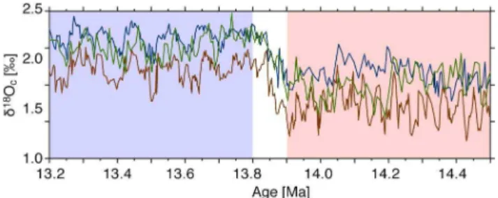
(Shevenell et al., 2004; Holbourn et al., 2005) show a mean increase of approximately 0.5‰ for this transition (Fig. 1).
Fig. 1. Compilation of high-resolution benthicδ18Ocrecords for
the Middle Miocene. The two records from Holbourn et al. (2005) are plotted in blue (Site 1237) and red (Site 1146). Another ODP record (Site 1171), at latitudes closer to Antarctica, is indicated in green (Shevenell et al., 2004) on the same time scale. The mean difference for every record from the period before (13.9–14.5 Ma) to after (13.2–13.8 Ma) the transition is approximately 0.5‰.
very small. The methods used to reconstruct paleo-pCO2 levels (e.g. alkenones, Pagani et al., 2005, stomatal index, K¨urschner et al., 2008, and boron isotopes, Pearson and Palmer, 2000; Demicco et al., 2003) involve large uncertain-ties. Furthermore, the different methods result in values that differ by more than 100–200 ppm amongst each other, indi-cating even larger errors than those assigned to the individual reconstructions.
We first explore the stability of the modeled Antarctic ice sheet under a large range of pCO2 levels in order to de-terminepCO2-thresholds for which the Antarctic continent glaciates and deglaciates (hysteresis experiments). Secondly, the ice-sheet response to variations in insolation is investi-gated by keeping thepCO2at a constant level. Thirdly, the combined effect of varyingpCO2and insolation forcings on the ice-sheet size are assessed.
2 Methods and experimental set-up 2.1 Ice sheet-climate model
In this study, we used a coupled ice sheet-climate model. The ice-sheet component has previously been applied to study Quaternary Northern Hemisphere glaciations (Sima, 2005; Sima et al., 2006). We changed the model set-up to an Antarctic configuration, forced only bypCO2and insolation. Furthermore we extended the model by including important climatic feedbacks.
The climate component consists of three large-scale boxes covering the entire southern hemisphere: a low (0–30◦S), middle (30–60◦S) and high (60–90◦S) latitude box (Fig. 2). The forcing consists of seasonal orbital forcing based on Laskar et al. (2004) combined with prescribed atmospheric pCO2levels. In the large-scale boxes of the climate model, energy is conserved and redistributed by meridional energy transport, taking into account the latent heat fluxes due to
Fig. 2. Set-up of the model. Upper: Large-scale box model con-sisting of low (0–30◦S), middle (30–60◦S) and high (60–90◦S) latitude cells. Each compartment is forced by shortwave (SW) and longwave (LW) radiation at the top of the atmosphere and sensible heat transport by eddies (H T), as well as latent heat transport in-duced by evaporation and snowfall (LH). The two lower latitude boxes are described by one general temperature (T) and albedo (α). Lower: The high-latitude, Antarctic box is subdivided into smaller grid cells with a resolution of 0.5◦in latitude. For each cell the en-ergy and mass balances are solved for surface and atmospheric tem-peratures (Ts andTa, respectively). Fluxes include incoming and
outgoing shortwave radiation at the top of atmosphere (SWa) and
at the land/ice/snow surface (SWs); reflected longwave radiation at
the top of atmosphere (LWa); longwave (LW), sensible heat (SH)
and latent heat of evaporation (LHeva) fluxes between the surface and atmosphere; latent heat of snowfall in atmosphere (LHsnow); heat flux into underlying bedrock (Fs). In all boxes ice flow
veloc-ities and ice height are computed, depending on the mass balance, local temperature (T), albedo (α) and isostasy.
The atmospheric and surface energy balances include pa-rameterizations for short- and long-wave radiation, latent heat of evaporation and snowfall, sensible heat exchange, heat flux into the surface and energy used by melting of ice and snow (Pollard, 1982, 1983; Jentsch, 1987, 1991; Wang and Mysak, 2000). Total snow accumulation and its latitu-dinal distribution is tuned to the present-day (total) Antarc-tic accumulation. The parameterization for snowfall de-pends on surface temperature, distance from the coast, sur-face height and daily sursur-face temperature (Oerlemans, 2002, 2004). Therefore, it includes important processes such as the elevation-desert effect (Pollard, 1983).
The ice-sheet model is symmetric around the South Pole. Within the ice sheet, flow velocities and temperatures are computed with a vertical resolution of 12 layers. The alti-tude and ice thickness of every latialti-tude grid cell are derived by solving the continuity equation using basal melting, local bedrock isostasy and a surface mass balance (Sima, 2005; Sima et al., 2006). The initial ice-free bedrock topography is reconstructed using the BEDMAP project database (Lythe et al., 2000) for bedrock elevation and ice thickness, con-sidering local isostasy. For the axially symmetric ice-sheet model, the high spatial resolution of the dataset is reduced, averaging the topography into the 0.5◦wide latitude bands. The initial bedrock used by the model is a simplified ver-sion of the zonally-averaged topography that includes a bulge close to the continental shelf and a flatter hinterland, resem-bling East Antarctica. Although no separate ocean compo-nent is included in the model, the energy and mass balances within the Antarctic box include the albedo of (seasonally varying) sea-ice. This is parameterized depending on the near-surface temperature of the appropriate grid cells. The surface albedo of the Antarctic continent depends on the ice and snow content of the corresponding grid cell and com-bines albedos of land (0.3), ice (0.35) and snow (0.75). A more detailed description of the climate forcing can be found in the Appendix.
2.2 Climate sensitivity of the model
The equilibrium climate sensitivity as estimated from 19 dif-ferent atmospheric general circulation models ranges from 2.1 to 4.4◦C, with an average of 3.2◦C (Randall et al., 2007). These models do not include a dynamic ice-sheet component, but do account for changes in snow cover and albedo. To tune the climate sensitivity of our model, we first ran the coupled ice sheet-climate model for the last 100 ka with constant pre-industrialpCO2of 280 ppm and varying orbital parameters. The modeled present-day ice sheet is in equilibrium with the radiative forcing and has a volume of 25.0×10¹⁵m3, similar to its estimated present-day size (e.g. Huybrechts et al., 2000; Oerlemans, 2002; Huybrechts, 2004). The mean hemispheric surface temperature is 14.9◦C. We deliberately enhanced the model sensitivity to changes inpCO2 in order to account for the missing water vapor feedback (see Appendix). In the
tuned model, a doubling ofpCO2 while maintaining fixed ice-sheet height and (seasonal) insolation distribution results in a hemispheric mean temperature increase of 2.5◦C. This value falls within the range of the values reported by the IPCC report (2007). The largest increase is found in atmo-spheric and surface temperatures in the Antarctic high lati-tude box, with values up to 3.9 and 4.4◦C, respectively. This polar amplification is due to the included ice-albedo feed-back and is comparable to pCO2-doubling simulations in comprehensive climate models (e.g. Masson-Delmotte et al., 2006a,b).
2.3 Insolation andpCO2forcings
Based on Earth’s orbital elements as computed by Laskar et al. (2004) we calculated daily insolation (Berger, 1978a,b) at the top of the atmosphere (for every latitude box) and at the surface for the high resolution Antarctic cells (60–90◦S). We used two different averages for comparison to ice-volume variations: annual mean and caloric summer (half-year of highest values) insolation. Since the atmospheric CO2level in the Middle Miocene is not very well constrained, the model was forced by prescribed scenarios of constantpCO2 and by a constant decrease inpCO2.
2.4 Experimental set-up
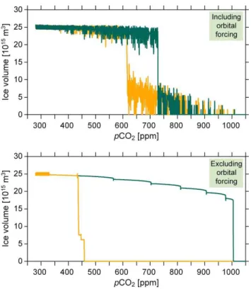
Firstly, hysteresis experiments were carried out in order to findpCO2-threshold values at which the Antarctic continent (de)glaciates. Two experiments were performed, one with and one without orbital forcing. The former started at 35 Ma at apCO2level of 1120 ppm. After slowly decreasingpCO2 to 280 ppm (reached at 20 Ma),pCO2was increased again to 1400 ppm (at 0 Ma). Because of this very slow decrease, the timing of the orbital parameters is not very important and the results would be similar if the experiments had started earlier or later. The latter experiment followed a similar scheme, but started with 560 ppm at 20 Ma. pCO2of 280 ppm was reached at 15 Ma and was increased to 1120 ppm at 0 Ma. In this case the timing is irrelevant, because the orbital parame-ters were fixed to present-day. In both experiments, the rate ofpCO2decrease as well as increase was 280 ppm/5 Ma (as in Pollard and DeConto, 2005) and ice volume is considered to be close to equilibrium.
Secondly, different levels of constant atmospheric CO2 were applied for model runs of a 1 Ma period, from 14.2 to 13.2 Ma (preceded by a 100 ka long spin-up time). This allows investigation of the effect of insolation fluctuations on ice-sheet volume under different constantpCO2conditions. The range between 300 and 1100 ppm was investigated in steps of 50 ppm with an increased resolution of 10 ppm from 590 to 650 ppm.
Fig. 3.Hysteresis experiment. Starting from no-ice conditions and highpCO2(orange) or starting from full ice sheet and lowpCO2 (green). Upper panel shows hysteresis including orbital forcing, lower panel without orbital variations. Rate of pCO2 change is 280 ppm/5 Ma.
ran from 14.1 to 13.7 Ma (without spin-up time) with varying insolation.
In all experiments daily insolation as a function of latitude was applied. The computations were performed at a daily time-step.
3 Results
3.1 Hysteresis experiments
To assess the sensitivity of the simulated ice volume topCO2 changes and to find the critical range of pCO2 at which the Antarctic continent (de)glaciates, two types of hystere-sis experiments were performed. The first included orbital variations, whereas the second was only forced by atmo-spheric CO2 (Fig. 3). In the former case of including or-bital variations, the (rapid) transition into a large ice sheet occurred around 615 ppm, preceded by a semi-stable small ice sheet. Orbital forcing acts as noise, therefore the ice sheet deglaciated under a relatively lowpCO2 when this was in-cluded (∼725 ppm), resulting in a small hysteresis window of approximately 110 ppm. In the latter case, where the or-bital variations were omitted, glaciation and deglaciation
oc-Fig. 4.ConstantpCO2experiments in the Middle Miocene (14.2– 13.2 Ma). Upper: Resulting ice-volume variations of four typical
pCO2forcing (280 ppm (black), 590 ppm (blue), 620 ppm (green) and 640 ppm (red)). Lower: Mean ice volume (dot) and standard deviation (arrows) of large (black/blue) and small (red) ice sheets, defined by theirpCO2level. The blue rectangle shows the Middle Miocene glaciation period as indicated by oxygen-isotope records.
curs at∼436 and 1004 ppm, respectively, accounting for a much larger hysteresis window of∼568 ppm. The modeled rate ofpCO2change was slow at 280 ppm/5 Ma, similar to the experiments of Pollard and DeConto (2005).
3.2 ConstantpCO2experiments
The criticalpCO2 for glaciation is around 615 ppm, when including orbital forcing. Below this threshold the entire Antarctic continent glaciates, with mean ice volumes be-tween 23 and 25×1015 m3 (Fig. 4). Between ∼640 and
∼700 ppm small ice sheets exist (almost) continuously over the entire modeled period. Higher pCO2 levels result in small, ephemeral ice sheets. Under constantpCO2forcing and insolation derived from Middle Miocene orbital param-eters (between 14.2 and 13.2 Ma) either large or small ice sheets occurs (Figs. 4 and 5). Only constantpCO2 values close to the threshold of 615 ppm cause a transition between these two states. Using constant 620 ppm forcing, Antarctica glaciates at 13.43 Ma.
The small ice sheets show large variations in ice vol-ume, up to∼2.3×10¹⁵ m3 for constantpCO2of 640 ppm. The volume of large ice sheets vary less under constant pCO2 conditions, with a maximum standard deviation of
∼1.0×10¹⁵ m3forpCO2values close to the threshold and nearly no variance at lower pCO2 levels. Two runs with constantpCO2close to the glaciation threshold and maxi-mum ice-volume variability are used to represent the large ice sheet (590 ppm) and the small ice sheet (640 ppm).
Fig. 5. Cross-section of large (left) and small (right) Antarctic ice sheets. Color scale corresponds to annual mean ice temperatures.
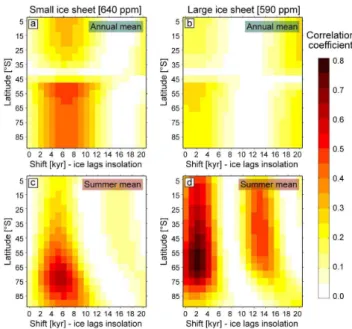
of southern latitude (Fig. 6). Variations in volume of both the large and small ice sheet correlate better to high (max-imum around 70◦S), than to low latitudes. In the case of the large ice sheet, the highest correlation coefficients are reached when ice volume lags insolation by approximately 2 ka. Maximum correlation coefficient values are 0.28 and 0.78 for annual and summer mean insolation, respectively. The small ice sheet matches insolation averages best for a lag of 5–6 ka. Maximum correlation coefficients for annual and summer mean insolation are 0.49 and 0.62, respectively. 3.3 VaryingpCO2experiments
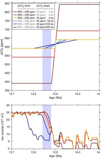
The first sensitivity test focusses on initial and finalpCO2 levels. In this set of experiments atmospheric CO2decreases linearly at a rate of 50 ppm/ka (Fig. 7 – yellow to red curves). In every experiment, the mid-point of the pCO2 drop oc-curs at the same moment in time (13.9 Ma), varying only the initial and finalpCO2 levels. The resulting ice volume transitions occur at about the same time, whereby the largest difference inpCO2forces the most rapid ice-sheet transition (Fig. 7 – red curve). Repeating the experiment for different slopes of thepCO2 transition gives practically identical re-sults (not shown).
The second test investigates the effect of the rate at which the atmospheric CO2 decreases during ice-sheet growth (Fig. 7 – blue curves). Experiments forced by a slow decrease inpCO2result in a variable duration of ice-sheet transition, between 20–30 ka. In runs with a rapid pCO2 drop, the transition length is independent of thepCO2drawdown rate. This relation also holds for different timings of thep CO2-transition (not shown).
In the last set of sensitivity experiments, the forcing is ap-plied at different moments in time resulting in different tim-ing of the ice-sheet expansion (Fig. 8).
4 Discussion
4.1 Hysteresis experiments
In the hysteresis experiment including Miocene orbital variations, a glaciation pCO2-threshold of approximately
Fig. 6. Ice-sheet variations correlated to insolation at latitudes be-tween 0 and 90◦S. Insolation is shifted backwards in time by 1 ka on horizontal axis (ice volume lags insolation). Correlation coeffi-cients are given for a small (aandc) and large (bandd) ice sheet and for annual (a and b) and summer mean (c and d) insolation. Best correlation is found for latitudes around 70◦S and a shift of 5– 6 ka (small ice sheet) or 2 ka (large ice sheet). Highest correlation coefficients for a small ice sheet are 0.49 and 0.62, for annual and summer mean insolation, respectively. Maxima for a large ice sheet are 0.28 (annual) and 0.78 (summer mean insolation).
615 ppm is found. The Antarctic ice sheet deglaciates when thepCO2increases by another∼110 ppm (at∼725 ppm). Annual mean temperatures over Antarctica differ by approxi-mately 2.5◦C between the glaciation and deglaciation thresh-olds. This hysteresis window is slightly smaller than in sim-ulations with the ice-sheet model of Pollard and DeConto (2005) (∼120 ppm), but similar to the computations of Huy-brechts (1993). The latter author proposed a range in hys-teresis width varying between ∼1 and 5◦C depending on the initial bedrock topography. Using a present-day orbital setting, Antarctic glaciation and deglaciation occurs under
∼435 and ∼1005 ppm, respectively (Fig. 3). This much larger hysteresis window is consistent with the findings of Pollard and DeConto (2005). Nevertheless, the synthetic set of orbital parameters applied by DeConto and Pollard (2003) and Pollard and DeConto (2005) resulted in a less extreme insolation variation than the orbital parameters used in this study (following Laskar et al., 2004). Indeed, when applying the DeConto and Pollard (2003) set of orbital parameters the hysteresis window increases to approximately 140 ppm (not shown).
Fig. 7. pCO2 sensitivity experiments – level of initial and final
pCO2(yellow to red colors) and rate ofpCO2decrease (blue col-ors). Colors in upper panel showpCO2forcing and correspond to ice-volume transition in lower panel. Blue box indicates approx-imate Antarctic glaciation as retrieved from sedimentary records. Glaciation is independent from initial and finalpCO2levels (red to orange). On the contrary, the rate of thepCO2drawdown is impor-tant. Extremely slow drop inpCO2(dark blue) results in delayed ice-sheet extension, relatively slow decrease (light blue) causes ap-propriate timing with glaciation. ApCO2drop of 50 ppm/50 ka or faster (for example 50 ppm/4 ka in orange) gives the same ice-sheet transition as 50 ppm/50 ka.
Pollard and DeConto, 2005). These show glaciation and deglaciation thresholds under much higher Antarctic temper-atures (10–20◦C higher than present-day, Huybrechts, 1993) or higherpCO2levels (∼780 and∼900 ppm, DeConto and Pollard, 2003). Although the values of DeConto and Pollard (2003) and DeConto et al. (2008) apply well to the Eocene-Oligocene transition, it is unlikely thatpCO2 levels in the Middle Miocene declined from values above ∼780 ppm. The relatively low glaciation threshold modeled in this study
Fig. 8. pCO2sensitivity experiment – timing ofpCO2decrease. Colors in(a)show pCO2 forcing and correspond to ice-volume transition in(b). Blue box indicates approximate Antarctic glacia-tion as found in sedimentary records. Green/orange curves result from fastpCO2transition (50 ppm/4 ka); purple/blue ones from a slow drop (50 ppm/200 ka). Black (gray) text in legend indi-cates best (not) fitting solutions (see Discussion section). Orange and dark blue curves correspond to their counterparts in Fig. 7.(c)
Annual mean insolation at 70◦S.(d) Summer mean insolation at 70◦S.
is much closer to thepCO2-reconstructions for the Middle Miocene (e.g. Pearson and Palmer, 2000; Demicco et al., 2003; Pagani et al., 2005; K¨urschner et al., 2008).
resulting hysteresis window shifted to lowerpCO2-values, with a glaciation threshold of approximately 400 ppm and a deglaciation around 425 ppm.
The modeled glaciation threshold value also depends on the initial bedrock topography. Huybrechts (1993) showed that the difference in Antarctic mean temperature between a flat and an unloaded present-day bedrock topography is approximately 8◦C, with higher bedrock elevations glaciat-ing at higher temperatures. The initial bedrock topography used in this study has elevations in between these extreme bedrock scenarios. Increasing the initial topography would probably cause an Antarctic glaciation under higherp CO2-values. The exact effects should be investigated in a bedrock-sensitivity study, which is beyond the scope of this study.
Another modeled process possibly affecting the glaciation threshold is the mass balance computation. The ice sheet-climate model lacks an interactive hydrological model. The total accumulation and its latitudinal distribution is tuned to values describing the present-day Antarctic ice sheet and de-pends on distance to the South Pole, surface height and daily surface temperature. However, if other factors have a large impact on the local mass balance and were significantly dif-ferent in the past, the glaciation threshold might be difdif-ferent. In summary, thepCO2threshold values could be slightly different than presented above, mainly depending on the ini-tial bedrock topography. If the climate sensitivity and the hy-drological cycle were significantly different in the past, these would also affect the threshold values.
4.2 ConstantpCO2experiments
Two types of stable ice sheets occur under the large range ofpCO2-levels investigated (Fig. 4). Small ice sheets show large ice-volume variations, where obliquity and precession are the dominant frequencies. On the other hand, large ice sheets reveal smaller ice-volume variations. These small fluctuations have a stronger influence of precession over obliquity and are therefore stronger correlated to summer in-solation than to annual mean inin-solation (Fig. 6). Huybers and Tziperman (2008) found a comparable relation between the ice-sheet size and the dominant frequencies for a Northern Hemisphere Pliocene ice sheet. They proposed that in the warm climate conditions under which thin (small) ice sheets occur, a long ablation season can counterbalance the oppo-site effect precession has on summer and fall insolation. The higher insolation intensity is then counteracted by a shorter summer duration. This effect reduces the precession signal in the ice-volume variations, and the obliquity becomes the dominant frequency. Raymo and Niscancioglu (2003) pro-posed that the obliquity signal is the result of variations in the insolation gradient between low and high latitudes, caus-ing variations in the meridional moisture and heat fluxes. However, our results show a strong obliquity frequency in the ice volume without explicitly calculating a moisture flux between low and high latitudes. Our modeled obliquity could
be caused by the opposing effects of insolation intensity and duration (as proposed by Huybers and Tziperman, 2008), be-cause we included daily insolation in the ice sheet-climate model. In large ice sheets the ablation period is too short to be influenced by this effect.
The difference in time lag between ice volume and inso-lation (5–6 ka for a large ice sheet versus 2 ka for a small ice sheet) is probably also related to the different frequen-cies dominating the ice-volume variations. Large ice sheets appear to be closer to resonance with the precessional forc-ing and therefore show a small time lag. Small ice sheets follow precessional forcing less closely, which explains the large time lag to insolation forcing.
The Antarctic ice-sheet expansion largely depends on a strong minimum in (summer) insolation (see next section), indicating a dependence on the insolation intensity, not on the summer duration.
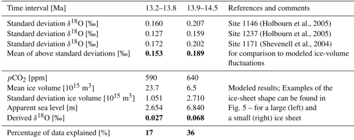
Under constant pCO2, the small ice sheets show much larger variations in volume than the large ice sheets. This can partly be observed in the oxygen-isotope record (Table 1). An F-test shows that the variance of the original oxygen-isotope data in the restricted time domains is significantly different (significance level of 90%). This difference might be explained by the fact that small ice sheets are more easily perturbed by changes in the forcing. Additionally, ablation plays a major role in ice-volume variations and occurs on two sides of the small ice sheet, whereas the large ice sheet only has an ablation zone at the outer rim (Fig. 5).
Correlations between continental ice volume and the oxy-gen isotopic composition of seawater vary around 1‰ for 100 m sea-level change (e.g. Fairbanks and Matthews, 1978; Schrag et al., 1996; Zachos et al., 2001). Using the present ocean area (3.6×10⁶km2) and the densities of water and ice (1000 kg/m3and 910 kg/m3, respectively), an apparent sea-level drop of 100 m is equivalent to ice build-up with a vol-ume of approximately 40×1015 m3. The ice-volume varia-tions in the large and small ice sheet result in sea-level fluctu-ations of 2.654 and 6.840 m, respectively (Table 1). This cor-responds toδ18O variations of 0.027 and 0.068‰. Accord-ingly, the fluctuations in the modeled ice-volume records can explain∼17 and∼36% of the variations found in the benthic oxygen-isotope records. The calibration does not account for variations inpCO2and does not take care of any effects caused by changes in (deep sea) temperature, salinity, local runoff, oxygen-isotope ratio of the ice, etc. Notwithstanding the crude calibration, the correlation between the standard deviations of data- and model-derived oxygen-isotope ratios is high.
The synchronous eccentricity and obliquity minima at
Table 1.Standard deviation of benthic oxygen-isotope records (cf. Shevenell et al., 2004; Holbourn et al., 2005) compared to the standard deviation derived from the modeled ice volume of the example constantpCO2experiments. Typical large ice sheet exists under 590 ppm (Fig. 5 – left); typical small ice sheet is found under a constantpCO2of 640 ppm (Fig. 5 – right).
Time interval [Ma] 13.2–13.8 13.9–14.5 References and comments
Standard deviationδ18O [‰] 0.160 0.207 Site 1146 (Holbourn et al., 2005) Standard deviationδ18O [‰] 0.127 0.159 Site 1237 (Holbourn et al., 2005) Standard deviationδ18O [‰] 0.172 0.202 Site 1171 (Shevenell et al., 2004) Mean of above standard deviations [‰] 0.153 0.189 for comparison to modeled ice-volume
fluctuations
pCO2[ppm] 590 640
Mean ice volume [1015m3] 23.7 6.5 Modeled results; Examples of the Standard deviation ice volume [1015m3] 1.051 2.710 ice-sheet shape can be found in Apparent sea level [m] 2.654 6.840 Fig. 5 – for a large (left) and Derivedδ18O [‰] 0.027 0.068 a small (right) ice sheet Percentage of data explained [%] 17 36
for an Antarctic glaciation at that time. Only constant at-mospheric CO2 levels at or very close to the threshold of 615 ppm can induce a transition from small to large ice vol-ume (Fig. 4). However, the modeled timing of the transi-tion occurs∼450 ka later than the transition identified from oxygen isotope records. Therefore, in order to glaciate the Antarctic continent at the right moment in time, a decrease inpCO2seems unavoidable (as previously proposed by Hol-bourn et al., 2005).
All high-resolution oxygen-isotope records (Shevenell et al., 2004; Holbourn et al., 2005) show a mean increase of approximately 0.5‰ from the period before (13.9–14.5 Ma) to the period after (13.2–13.8 Ma) the rapid transition (see also Fig. 1). The two stable large and small ice-sheet sim-ulations around the pCO2-threshold have average ice vol-umes of ∼23.7 and ∼6.5×10¹⁵ m3. ApCO2-decline be-tween these two states would result in a sea level differ-ence of∼43.3 m. This sea-level drop would increase the oxygen-isotope ratio of sea water by approximately 0.43‰. This suggests that more than 85% of the Middle Miocene oxygen-isotope transition found in the sedimentary records can be explained by ice-volume expansion on Antarctica. In future research this comparison will be further investigated by including oxygen isotopes directly in the ice sheet-climate model.
4.3 VaryingpCO2experiments
The first sensitivity test (see Sect. 3.3) showed that a larger difference between initial and finalpCO2forcing resulted in a faster ice-sheet expansion. This can be explained by the different variability of the ice sheet at differentpCO2 lev-els. The larger standard deviations of 1.051×10¹⁵ m3 and 2.710×10¹⁵ m3 (Table 1) in the 590 and 640 ppm runs, re-spectively, increase the probability for insolation variations
to act against a rapid ice-volume transition. The sedimentary records do not indicate such a rapid glaciation (e.g. Shevenell et al., 2004; Holbourn et al., 2005), but do show large vari-ability in time (Fig. 1). Furthermore, under highpCO2levels hardly any ice covered the Antarctic continent (Fig. 4 and 7). Previous studies (e.g. Pekar and DeConto, 2006) did show evidence for a dynamic ice sheet shortly before the Middle Miocene. Therefore, the relatively small difference inpCO2 between 640 and 590 ppm, crossing the threshold value of
∼615 ppm, was used in the remaining sensitivity experi-ments.
The second sensitivity test dealt with the slope of the at-mospheric CO2 drawdown (Fig. 7 – blue curves). The du-ration of the ice-sheet transition was defined as the period in which ice volume is larger than the maximum volume of the small ice sheet and smaller than the minimum size of the large ice sheet. Additional experiments showed that the slow forcing did not have a strong effect on the duration of the ice-sheet expansion. The duration merely depended on the timing of thepCO2drop. This quite constrained timing (see next paragraph) limited the glaciation event to a length of approximately 30 ka, comparable to the time interval of 30– 40 ka derived fromδ18O records (cf. Holbourn et al., 2005).
The third set of sensitivity experiments investigated the timing of the pCO2 decrease for 50 ppm/200 ka and for 50 ppm/4 ka (Fig. 8). The best fit to δ18O data (glacia-tion time shown by blue box) occurred when the simula(glacia-tions crossed thepCO2threshold of approximately 615 ppm be-tween∼13.90 and∼13.93 Ma.
during minima in summer insolation. For a modeled ice-sheet expansion to occur in the Middle Miocene at the same time as indicated by the shift to heavier benthic oxygen-isotope ratios in the sedimentary records, the minimum in high-latitude summer insolation at approximately 13.89 Ma appears to be the most suitable candidate for triggering the transition. A clear example is the experiment of fastpCO2 decrease at 13.925 Ma (Fig. 8 – yellow curve), where an increasing insolation opposed ice growth. Only when the summer insolation reached the minimum of∼13.89 Ma, the ice volume expanded. Our results suggest 13.89 Ma as a more important insolation moment for the Antarctic glacia-tion than the previously suggested 13.84 Ma. These experi-ments were based on a 50 ppm difference inpCO2, but ex-tending this range would give similar results (see first sensi-tivity test).
The comparison of the three sensitivity experiments to high-resolution oxygen-isotope records indicates thatpCO2 should drop below the threshold of∼615 ppm just before the ice-sheet transition (as suggested by Holbourn et al., 2005). Most probably the initial and finalpCO2levels were close to the threshold values, otherwise the variation in the ice-sheet volume was extremely small or even no ice was cov-ering the Antarctic continent. The exact timing of the ice-sheet expansion depends largely on the orbital parameters, where the minimum of summer and annual mean insolation at∼13.89 Ma takes a key position.
5 Conclusions
Despite the relatively simple geometry of our ice sheet-climate model, the realistically tuned sheet-climate sensitivity and hysteresis experiments allows us to conclude that the mech-anism described below is robust. However, exact values are model dependent and should only be taken as a guideline.
1. It is very unlikely that a constant pCO2 in combina-tion with orbital forcing induced the large-scale Antarc-tic glaciation in the Middle Miocene. Constant levels produced either a large (below∼610 ppm) or a small (above∼630 ppm) ice sheet. Modeled ice volume had a smaller ice-volume standard deviation than expected from benthic oxygen-isotope records. The residual vari-ation in these isotope records probably originate from fluctuations inpCO2and other changes in climatic or local conditions.
2. The extent of thepCO2 drawdown was not important for the timing or duration of the glaciation transition, as long as it crossed the∼615 ppm threshold. Moderate or quickpCO2 reductions resulted in comparable and realistic ice-sheet extension. The timing of thepCO2 decrease was important, because favorable orbital pa-rameters enhanced the ice-sheet expansion. In order to expand the Antarctic ice sheet in the appropriate time
interval as indicated by benthic oxygen-isotope records (13.84–13.88 Ma) thepCO2threshold must have been crossed between∼13.90 and∼13.93 Ma.
3. After the decrease inpCO2 the minimum in summer insolation restricted the timing of ice growth on Antarc-tica. Therefore, the main ice-sheet expansion probably started around 13.89 Ma.
Appendix A Model description
The ice sheet-climate model is controlled by energy and mass balances. Orbital elements are derived following the work of Laskar et al. (2004). They drive the seasonal solar radia-tion at the top of the atmosphere and define, together with thepCO2, the amount of energy entering the entire climate system.
A1 Energy and temperature balances
The model consists of three large-scale boxes covering the entire southern hemisphere: a low (0–30◦S), middle (30– 60◦S) and high (60–90◦S) latitude box (Fig. 2). Within the climate system energy is conserved and changes in time are described by (Pollard, 1983; Hartmann, 1994):
∂Eao
∂t =RTOA−1Fao+LH (A1)
whereEaois the total energy in the system,tthe time,RTOA the net incoming solar radiation at the top of the atmosphere, 1Fao the divergence of the meridional energy transport in the ocean as well as in the atmosphere, andLH the latent heat added to the atmosphere after condensation and freezing of water vapor. The net incoming radiation is the sum of the incoming short-wave radiation (SWp) and the outgoing
short- and long-wave radiation (LWp): RTOA=SWp↓−SWp↑−LWp↑.
Radiation fluxes in the twolower latitudeboxes (0–30◦S and 30–60◦S) are parameterized as:
SWp↓−SWp↑=Q(1−αp) LWp↑=εpσ Ta4+fCO2
whereQis the solar insolation at the top of the atmosphere, αp the planetary albedo,εp the planetary emissivity andσ
the Stefan-Boltzmann constant.Tais interpreted as the
near-surface air temperature andfCO2 as the effect of the
atmo-spheric CO2content (cf., Myhre et al., 1998):
fCO2 = −8
ln(CO2
280)
Therefore, a doubling ofpCO2from 280 ppm (pre-industrial conditions) to 560 ppm accounts for a reduction of 8 W/m2 in the outgoing longwave radiation of the two lower lati-tude boxes, accounting not only forpCO2, but also for other greenhouse gases (mainly water vapor, see Sect. A4).
The physical processes in thehigh latitudebox are deci-phered in much higher resolution and complexity. For every 0.5◦ latitude energy and mass balances for the atmosphere and for the surfaces are simultaneously solved. Atmospheric temperature (Ta) is described by:
Ca dTa
dt =Ra+LW+SH+LHeva+LHsnow
and surface temperature (Ts) by: Cs
dTs
dt =Rs −LW−SH−LHeva−Fs−Fm
whereCa,s is the heat capacity for the atmosphere and
sur-face, respectively.
The incoming energy at the top of the atmosphere and at the surface is represented as (Jentsch, 1987; Wang and Mysak, 2000):
Ra=SWa↓−SWa↑−LWa↑
=Q(1−αa)(1−τ )(1+τ αs)−(ε2σ Ta4+(1−ε1)σ Ts4)
Rs =SWs↓−SWs↑
=τ Q(1−αa)(1−αs)
whereτ is the atmospheric transmissivity of solar radiation, αa,s the atmospheric and surface albedos, ε2 an emissivity constant andε1a term describing the greenhouse effect (see below).
The longwave and sensible heat fluxes between the atmo-sphere and surface are parameterized as:
LW =σ Ts4−ε1σ Ta4
SH=λ(Ts−Ta)
whereλis a heat exchange coefficient which in principle de-pends on wind speed, atmospheric density and heat capacity, but is taken to be constant. The heat flux into the subsurface soil or upper ice layer (Fs) is given by:
Fs =
2k1 1z1
(Ts −Ta)
wherek1is the thermal conductance of snow and 1z1 the depth range of conduction.
The latent heat due to evaporation (LHeva) is parameter-ized as (Hartmann, 1994):
LHeva=ρairLvCDEU[qs∗(1−RH)+
RH Be
cp Lv
(Ts−Ta)]
whereρairis the air density,Lvis the latent heat of
vapora-tion,CDEan exchange coefficient,Uthe wind speed,qs∗the
sea surface humidity,Bethe equilibrium Bowen ratio,cpthe
specific heat of dry air and RH the relative humidity. The latent heat associated with snowfall (LHsnow) depends on the accumulation of snow:
LHsnow=LsA
whereLs is the latent heat of sublimation andAthe
accu-mulation. The snow is considered to be evaporated in the low latitude box, accounting for theLH-term in the energy equation (Eq. A1). The total accumulation and its latitudinal distribution is tuned to the present-day total Antarctic accu-mulation and depends on the distance to the South Pole (r), the surface height (hsfc) and the daily surface temperature (Ts) (Oerlemans, 2002, 2004). It therefore includes processes
such as the elevation-desert effect (Pollard, 1983): A=(ca+cbr)e
−hsfc(r) cd eκTs
whereca,bare (tuning) constants,cdis a characteristic length
scale and κ a constant describing the precipitation depen-dence on temperature. Only when the local temperature is below 2◦C, snow is accumulated (Oerlemans, 2001).
The amount of energy available for melting (Fm) depends
on the incoming energy and the thickness and heat capac-ity of the top surface layer (Fraedrich et al., 2005). The af-fected layer is 20 cm deep (dtop) and consists of snow (dsnow), soil (dsoil) or a mixture of both. The heat capacity (Cs) used
for computation of the surface temperature is therefore com-puted by:
Cs =
CsnowCsoildtop
Csnowdsoil+Csoildsnow
The atmospheric and surface temperature equations are si-multaneously solved. Daily computation is necessary, be-cause the orbital cycle as well as processes of snow accumu-lation and melting have a strong seasonal imprint (Pollard, 1983). The meridional heat transport (1Feo) accounts for the coupling between the boxes, and is proportional to the temperature gradient based on the diffusion approximation (Sellers, 1970; North, 1975). The atmospheric temperatures, and also the surface temperatures, are further extrapolated to-wards their altitudes (hsfc) according to the prescribed lapse rate,Ŵlapse:
Ta=Ta+Ŵlapsehsfc(r).
A2 Mass balance
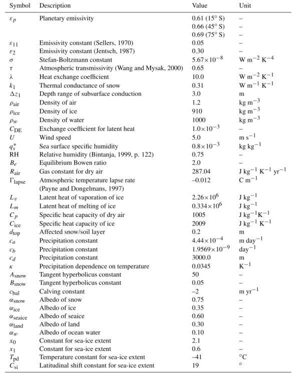
Table A1.List and desciption of constant parameters.
Symbol Description Value Unit
εp Planetary emissivity 0.61 (15◦S) –
0.66 (45◦S) – 0.69 (75◦S) –
ε11 Emissivity constant (Sellers, 1970) 0.05 –
ε2 Emissivity constant (Jentsch, 1987) 0.30 –
σ Stefan-Boltzmann constant 5.67×10⁻⁸ W m−2K−4
τ Atmospheric transmissivity (Wang and Mysak, 2000) 0.65 –
λ Heat exchange coefficient 10.0 W m−2K−1
k1 Thermal conductance of snow 0.31 W m−1K−1
1z1 Depth range of subsurface conduction 3.0 m
ρair Density of air 1.2 kg m−3
ρice Density of ice 910 kg m−3
ρw Density of water 1000 kg m−3
CDE Exchange coefficient for latent heat 1.0×10⁻³ –
U Wind speed 5.0 m s−1
qs∗ Sea surface specific humidity 0.8×10⁻³ kg kg−1 RH Relative humidity (Bintanja, 1999, p. 122) 0.75 –
Be Equilibrium Bowen ratio 2.0 –
Rair Gas constant for dry air 287.04 J kg−1K−1yr−1
Ŵlapse Atmospheric temperature lapse rate –0.012 C m−1 (Payne and Dongelmans, 1997)
Lv Latent heat of vaporation of ice 2.26×10⁶ J kg−1
Lm Latent heat of melting of ice 0.334×10⁶ J kg−1
Cp Specific heat capacity of dry air 1005 J kg−1K−1
Cice Specific heat capacity of ice 2009 J kg−1K−1
dtop Affected snow/soil layer 0.2 m
ca Precipitation constant 4.44×10⁻⁴ m day−1
cb Precipitation constant 1.9569×10⁻⁹ day−1
cd Precipitation constant 3000.0 m
κ Precipitation dependence on temperature 0.0345 K−1
Asnow Tangent hyperbolicus constant 50 –
Bsnow Tangent hyperbolicus constant 0.05 –
cbal Calving constant –2 m yr−1
αsnow Albedo of snow 0.75 –
αice Albedo of ice 0.35 –
αseaice Albedo of seaice 0.60 –
αland Albedo of land 0.30 –
αw Albedo of ocean water 0.10 –
x0 Constant for sea-ice extent 2.1 –
x1 Constant for sea-ice extent 0.6 –
Tpd Temperature constant for sea-ice extent –41 ◦C
Csi Latitudinal shift constant for sea-ice extent 19 ◦
The ice sheet is allowed to grow into the surrounding ocean as long as it is hydrostatically floating. When the total weight of the ice column exceeds the floating criteria, calving occurs (Pollard, 1982) and the total mass balance (G) will be set to a negative value (cbal):
G=cbalifρairhice< ρw(hsfc−hice)
whereρiceandρw are the densities of ice and water,
respec-tively,hiceis the ice thickness, andhsfc, the elevation of the
surface with respect to the current sea level, which is taken as a constant reference level. This crude calving parameteriza-tion also accounts for occurrence of proglacial lakes and/or marine incursions (Pollard, 1982).
Bottom melting (S) occurs when the temperature in the basal layer (Tbase) exceeds the pressure melting point (Tpmp):
S= Cice Lm
(Tbase−Tpmp) 1zbase
whereCiceis the specific heat of ice andLmthe specific
la-tent heat of fusion of ice and1zbasethe thickness of the basal layer.
A3 Albedo
A separate snow balance is computed to parameterize the surface albedo. The formulas for this cumulative balance re-semble the previous surface mass and energy balance equa-tions, except for the fact that the snow depth cannot become negative. The daily derived surface albedo (αs) depends on
the snow depth (dsnow), when the snow layer is thicker than 10 cm:
α= αsnow+αice
2
+ αsnow−αice
2 tanh(Asnow(dsnow−Bsnow))
where the slope (Asnow) and shift (Asnow) are constant and αsnowandαiceare the albedos of snow and ice, respectively. When there is less or no ice/snow, the land, ocean (low and middle latitude boxes) or sea-ice albedos (high latitude box) are used. The latitudinal extent of sea-ice (latsi) is given by (Jentsch, 1987):
latsi=sin−1[tanh(x0( Tpd
Ta
)x1)] −C
si
wherex0andx1are tuning constants,Tpda measure for the present-day value of sea-water temperature andCsia latitu-dinal shift.
The planetary (αp) and atmospheric (αa) albedos are
parameterized as functions of latitude (Wang and Mysak, 2000):
αp =0.6−0.4 cos(lat) αa=0.3−0.1 sin(lat).
A4 Greenhouse effect
The longwave radiation constantε1 accounts for the green-house effect due topCO2and other greenhouse gases: ε1=ε10+ε11
p
e′
where,e′is the atmospheric vapor pressure, related to the sat-uration specific humidity (qsat) and relative humidity (RH): e′=1.6×10³RHqsat
where: qsat=
1.57×10¹¹ ρairRairTa
e−5421Ta
withRairbeing the gas constant for dry air.
According to Staley and Jurica (1970) and Jentsch (1991), the CO2-emission factor can be parameterized by:
εCO2
10 =0.1+0.025ln(CO2). (A2)
The other main greenhouse gas, water vapor (H2O), also contributes about half to the (present-day) greenhouse effect. Because of the fact that we do not explicitly compute the hydrological cycle, this feedback can not be parameterized separately. To still include the effect of water vapor, we in-creased the climate sensitivity topCO2Eq. (A2) is therefore expanded and retuned to:
ε10=ε10CO2+ε10H2O=0.27+0.05ln(CO2).
A doubling of atmospheric CO2results in a climate sensitiv-ity of 2.5◦C and modeled present-day ice-sheet size, accumu-lation and temperature distribution are similar to estimates (Huybrechts et al., 2000; Oerlemans, 2002).
A5 List of constant parameters
Table A1 gives an overview of the parameters used in the ice sheet-climate model.
Acknowledgements. This project was funded by the DFG (Deutsche Forschungsgemeinschaft) within the European Graduate College “Proxies in Earth History”. We thank the three anonymous reviewers and the editor for their constructive comments.
Edited by: E. W. Wolff
References
Abels, H. A., Hilgen, F. J., Krijgsman, W., Kruk, R. W., Raffi, I., Turco, E., and Zachariasse, W. J.: Long-period orbital con-trol on middle Miocene global cooling: Integrated statigraphy and astronomical tuning of the Blue Clay Formation on Malta, Paleoceanography, 20, 2362–2367, doi:10.1029/2004PA001129, 2005.
Berger, A. L.: Long Term Variations of Caloric Insolation resulting from the Earth’s orbital elements, Quaternary Res., 9, 139–167, 1978a.
Berger, A. L.: Long Term Variations of Daily Insolation and Qua-ternary Climatic Changes, J. Atmos. Sci., 35, 2362–2367, 1978b. Bintanja, R.: The Antarctic ice sheet and climate, Ph.D. thesis,
Uni-versity of Utrecht, The Netherlands, 1999.
Coxall, H. K., Wilson, P. A., P¨alike, H., Lear, C., and Backman, J.: Rapid stepwise onset of Antarctic glaciation and deeper calcite compensation in the Pacific Ocean, Nature, 443, 53–57, 2005. DeConto, R. M. and Pollard, D.: Rapid Cenozoic glaciation of
Antarctica induced by declining atmospheric CO2, Nature, 42, 245–249, 2003.
DeConto, R. M., Pollard, D., Wilson, P. A., P¨alike, H., Lear, C. H., and Pagani, M.: Thresholds for Cenozoic bipolar glaciation, Na-ture, 455, 652–657, 2008.
Demicco, R. V., Lowenstein, T. K., and Hardie, L. A.: Atmospheric
pCO2since 60 Ma from records of seawater pH, calcium, and primary carbonate mineralogy, Geology, 31, 793–796, 2003. Fairbanks, R. G. and Matthews, R. K.: The Marine Oxygen Isotope
Flower, B. P. and Kennett, J. P.: Middle Miocene deep-water pa-leoceanography in the Southwest Pacific relations with East Antarctic ice-sheet development, Paleoceanography, 10, 1095– 1112, 1995.
Fraedrich, K., Jansen, H., Kirk, E., and Lunkeit, F.: The Planet Simulator: towards a user friendly model, Meteor. Zeitschrift, 14, 299–30, 2005.
Hartmann, D. L.: Global Physical Climatology, Academic Press, San Diego, 1994.
Holbourn, A., Kuhnt, W., Schulz, M., and Erlenkeuser, H.: Impacts of orbital forcing and atmospheric carbon dioxide on Miocene ice-sheet expansion, Nature, 438, 483–487, 2005.
Holbourn, A., Kuhnt, W., Schulz, M., Flores, J. A., and Ander-son, N.: Orbitally-paced climate evolution during the middle Miocene “Monterey” carbon-isotope excursion, Earth Planet. Sc. Lett., 261, 534–550, 2007.
Huybers, P. and Tziperman, E.: Integrated summer insolation forc-ing and 40,000-year glacial cycles: The perspective from an ice-sheet/energy-balance model, Paleoceanography, 23, PA1208, doi:10.1029/2007PA001463, 2008.
Huybrechts, P.: Glaciological modelling of the Late Cenozoic East Antarctic ice sheet: Stability or dynamism?, Geogr. Ann., 75, 221–238, 1993.
Huybrechts, P.: Antarctica, in: Mass balance of the cryosphere: observations and modelling of contemporary and future changes, edited by: Bamber, J. L. and Payne, A. J., 491–523, Cambridge University Press, Cambridge, United Kingdom, 2004.
Huybrechts, P., Steinhage, D., Wilhems, F., and Bamber, J.: Balance velocities and measured properties of the Antarctic ice sheet from a new compilation of gridded data for modeling, Ann. Glaciol., 30, 52–60, 2000.
Jentsch, V.: Cloud-ice-vapor feedbacks in a global climate model, in: Irreversible Phenomena and Dynamical Systems Analysis in Geosciences, edited by: Nicolis, C. and Nicolis, G., Reidel Pub-lishing Company, Dordrecht, The Netherlands, 1987.
Jentsch, V.: An Energy Balance Climate Model With Hydrological Cycle. 1. Model Description and Sensitivity to Internal Parame-ters, J. Geophys. Res., 96, 17 169–17 179, 1991.
K¨urschner, W. M., Kvacek, Z., and Dilcher, D. L.: The impact of Miocene atmospheric carbon dioxide fluctuations on climate and the evolution of terrestrial ecosystems, Proc. Nat. Acad. Sci. USA, 106, 449–453, 2008.
Laskar, J., Robutel, P., Joutel, F., Gastineau, M., Correia, A. C. M., and Levrard, B.: A long-term numerical solution for the insola-tion quantities of the Earth, Astron. Astrophys., 428, 261–285, 2004.
Lythe, M. B., Vaughan, D. G., and the BEDMAP Consortium: BEDMAP – bed topography of the Antarctic. 1:10 000 000 scale map, British Antarctic Survey, Cambridge, United Kingdom, 2000.
Masson-Delmotte, V., Dreyfus, G., Braconnot, P., Johnsen, S., Jouzel, J., Kageyama, M., Landais, A., Loutre, M.-F., Nouet, J., Parrenin, F., Raynaud, D., Stenni, B., and Tuenter, E.: Past temperature reconstructions from deep ice cores: relevance for future climate change, Clim. Past, 2, 145–165, 2006a.
Masson-Delmotte, V., Kageyama, M., Branconnot, P., Charbit, S., Krinner, G., Ritz, C., Guilyardi, E., Jourzel, J., Abe-Ouchi, A., Crucifix, M., Gladstone, R. M., Hewitt, C. D., Kitoh, A., LeGrande, A. N., Marti, O., Merkel, U., Motoi, T., Ohgaito, R.,
Otto-Bliesner, B., Peltier, W. R., Ross, I., Valdes, P. J., Vettoretti, G., Weber, S. L., Wolk, F., and Yu, Y.: Past and future polar am-plifications of climate change: climate model intercomparisons and ice-core constraints, Clim. Dynam., 26, 513–529, 2006b. Miller, K. G., Mountain, G. S., Browning, J. V., Kominz, M.,
Sugar-man, P. J., Christie-Blick, N. C., Katz, M. E., and Wright, J. D.: Cenozoic global sea level, sequences, and the New Jersey tran-sect: results from coastal plan and continental slope drilling, Rev. Geophys., 36, 569–601, 1998.
Miller, K. G., Kominz, M., Browning, J. V., Wright, J. D., Moun-tain, G. S., Katz, M. E., Sugarman, P. J., Cramer, B. S., Christie-Blick, N. C., and Pekar, S. F.: The Phanerozoic record of global sea-level change, Science, 310, 1293–1298, 2005.
Myhre, G., Highwood, E. J., Shine, K. P., and Stordal, F.: New es-timates of radiative forcing due to well mixed greenhouse gases, Geophys. Res. Lett., 25, 2715–2718, 1998.
North, G. R.: Theory of Energy Balance Climate Models, J. Atmos. Sci., 32, 2033–2043, 1975.
Oerlemans, J.: Glaciers and climate change, in: Modeling glacier mass balance, edited by: Oerlemans, J., chap. 4, Balkema, The Netherlands, 2001.
Oerlemans, J.: Global dynamics of the Antarctic ice sheet, Clim. Dynam., 19, 85–93, 2002.
Oerlemans, J.: Antarctic ice volume and deep-sea temperature dur-ing the last 50 Myr: a model study, Ann. Glaciol., 39, 13–19, 2004.
Pagani, M., Zachos, J. C., H., F. K., Tipple, B., and Bohaty, S.: Marked decline in atmospheric carbon dioxide concentrations during the Paleogene, Science, 309, 600–603, 2005.
Payne, A. J. and Dongelmans, P. W.: Self-organization on the ther-momechanical flow of ice sheets, J. Geophys. Res., 106, 12219– 12233, 1997.
Pearson, P. N. and Palmer, M. R.: Atmospheric carbon dioxide con-centrations over the past 60 million years, Nature, 406, 695–699, 2000.
Pekar, S. F. and DeConto, R. M.: High-resolution ice-volume esti-mates for the early Miocene: Evidence for a dynamic ice sheet in Antarctica, Palaeogeogr. Palaeocl., 231, 101–109, 2006. Pollard, D.: A simple ice sheet model yields realistic 100 kyr glacial
cycles, Nature, 296, 334–338, 1982.
Pollard, D.: A Coupled Climate-Ice Sheet Model Applied to the Quaternary Ice Ages, J. Geophys. Res., 88, 7705–7718, 1983. Pollard, D. and DeConto, R. M.: Hysteresis in Cenozoic Antarctic
ice-sheet variations, Global Planet. Change, 45, 9–21, 2005. Randall, D. A., Wood, R. A., Bony, S., Colman, R., Fichefet, T.,
Fyfe, J., Kattsov, V., Pitman, A., Shukla, J., Srinivasan, J., Stouf-fer, R., Sumi, A., and Taylor, K.: Climate Change 2007: The Scientific Basis, Contribution of Working Group 1 to the Fourth Assessment Report of the Intergovernmental Panel on Climate Change, edited by: Solomon, S., Qin, D., Manning, M., Chen, Z., Marquis, M., Averyt, K., Tignor, M., and Miller, H., p. 881, Cambridge University Press, Cambridge, United Kingdom and New York, NY, USA, 2007.
Raymo, M. E.: The initiation of northern hemisphere glaciation, Paleoceanography, 9, 399–404, 1994.
Raymo, M. E. and Niscancioglu, K.: The 41 kyr world: Mi-lankovitch’s other unsolved mystery, Paleoceanography, 18, 1011, doi:10.1029/2002PA000791, 2003.
con-straints on the temperature and oxygen isotopic composition of the Glacial Ocean, Science, 272, 1930–1932, 1996.
Sellers, W. D.: A global climate model based on the energy balance of the earth-atmosphere system, J. Appl. Meteorol., 8, 392–400, 1970.
Shevenell, A., Kenneth, J. P., and Lea, D. W.: Middle Miocene Southern Ocean cooling and Antarctic cryosphere expansion, Science, 305, 1766–1770, 2004.
Shevenell, A., Kenneth, J. P., and Lea, D. W.: Middle Miocene ice sheet dynamics, deep-sea temperatures, and carbon cycling: A Southern Ocean perspective, Geochem. Geophy. Geosy., 9, Q02006, doi:10.1029/2007GC001736, 2008.
Sima, A.: Modeling oxygen isotopes in ice sheets linked to Quater-nary ice-volume variations, Ph.D. thesis, University of Bremen, Germany, 2005.
Sima, A., Paul, A., Schulz, M., and Oerlemans, J.: Modeling the oxygen-isotope composition of the North American Ice Sheet and its effect on the isotopic composition of the ocean during the last glacial cycle, Geophys. Res. Lett., 33, L15706, doi: 10.1029/2006GL026923, 2006.
Staley, D. O. and Jurica, G. M.: Flux emissivity tables for water vapor carbon dioxide and ozone, J. Appl. Meteorol., 9, 365–372, 1970.
Van Tuyll, C. I., van de Wal, R. S. W., and Oerlemans, J.: The response of a simple Antarctic ice-flow model to temperature and sea-level fluctuations over the Cenozoic era, Ann. Glaciol., 46, 69–77, 2007.
Wang, Z. and Mysak, L. A.: A simple coupled atmosphere-ocean-sea ice-land surface model for climate and paleoclimate studies, J. Climate, 13, 1150–1172, 2000.
Zachos, J. C., Pagani, M., Sloan, L., Thomas, E., and Billups, K.: Trends, Rythms, and Aberrations in Global Climate 65 Ma to Present, Science, 292, 686–693, 2001.