Modeling geologically abrupt climate changes in the Miocene

(1)

CPD

6, 2687–2701, 2010

Modeling geologically abrupt

climate changes in the Miocene

B. J. Haupt and D. Seidov

Title Page

Abstract Introduction

Conclusions References

Tables Figures

◭ ◮

Back Close

Full Screen / Esc

Printer-friendly Version Interactive Discussion

Discussion

P

a

per

|

Dis

cussion

P

a

per

|

Discussion

P

a

per

|

Discussio

n

P

a

per

Clim. Past Discuss., 6, 2687–2701, 2010 www.clim-past-discuss.net/6/2687/2010/ doi:10.5194/cpd-6-2687-2010

Climate of the Past Discussions

This discussion paper is/has been under review for the journal Climate of the Past (CP). Please refer to the corresponding final paper in CP if available.

Modeling geologically abrupt climate

changes in the Miocene

B. J. Haupt1and D. Seidov2

1

EMS Earth and Environmental Systems Institute, Pennsylvania State University, PA 16802, University Park, USA

2

NOAA/NODC, Ocean Climate Laboratory, MD 20910, Silver Spring, USA

Received: 9 November 2010 – Accepted: 25 November 2010 – Published: 14 December 2010

Correspondence to: B. J. Haupt (bjhaupt@psu.edu)

(2)

CPD

6, 2687–2701, 2010

Title Page

Tables Figures

◭ ◮

Back Close

Full Screen / Esc

Discussion

P

a

per

|

Dis

cussion

P

a

per

|

Discussion

P

a

per

|

Discussio

n

P

a

per

|

Abstract

The gradual cooling of the Cenozoic, including the Miocene epoch, was punctuated by many geologically abrupt warming and cooling episodes – strong deviations from the cooling trend with time span of ten to hundred thousands of years. Our working hypoth-esis is that some of those warming episodes at least partially might have been caused

5

by dynamics of the emerging Antarctic Ice Sheet, which, in turn, might have caused strong changes of sea surface salinity in the Miocene Southern Ocean. Feasibility of this hypothesis is explored in a series of coupled ocean-atmosphere computer exper-iments. The results suggest that relatively small and geologically short-lived changes in freshwater balance in the Southern Ocean could have significantly contributed to at

10

least two prominent warming episodes in the Miocene. Importantly, the experiments also suggest that the Southern Ocean was more sensitive to the salinity changes in the Miocene than today, which can attributed to the opening of the Central American Isthmus as a major di_fference between the Miocene and the present-day ocean-sea geometry.

15

1 Introduction

The Miocene is a geological epoch extending from about 23 to 5.3 Ma and is a time of continuous cooling that began in the middle of the Cenozoic Era (Crowley and North, 1991; see recent update in Thomas, 2008). This long-term Paleogene cooling trend is thought to be caused by continuous decrease of atmospheric CO₂ (Pagani et al.,

20

2005; Shellito et al., 2003; Zachos et al., 2008). After opening of Drake Passage in the Oligocene and emerging of a paleo analog of the present-day Antarctic Circumpolar Current (ACC) – proto-ACC, climate cooling had accelerated (e.g., Barron and Peter-son, 1991; Bice et al., 2000; Seidov, 1986). The ocean-cryosphere interaction might have already then become a significant element of ocean circulation and climate.

(3)

CPD

6, 2687–2701, 2010

Title Page

Tables Figures

◭ ◮

Back Close

Full Screen / Esc

Discussion

P

a

per

|

Dis

cussion

P

a

per

|

Discussion

P

a

per

|

Discussio

n

P

a

per

The geological and glaciological reconstructions of early and middle Miocene expose prominent warm spikes and seal level rises around 22, 16, 14, and 12 Ma, coincident with strong excursions ofδ18O, e.g., Abreu and Anderson, 1998; Bush and Philander, 1997. These geologically short-lived departures from the main cooling trend are hard to explain in terms of the familiar greenhouse gases paradigm and call for looking at the

5

sea-ice interactions which have fitted the timing of those disturbances. This may make sense as the Miocene sea-level history suggests that ice sheets existed for geologi-cally short intervals (i.e., lasting about 100 000 years) even in the previously assumed ice-free Late Eocene (e.g., Miller et al., 2005). Far from being an only possible expla-nation, the dynamics of emerging of the Antarctic Ice Sheet could be a plausible one

10

specifically for short-term deglaciation episodes.

Understanding paleoclimate dynamics on geological scale is a very challenging task. In our case, straightforward computer simulations of entire Miocene Epoch are not fea-sible, neither currently nor in foreseeable future. Zooming onto much shorter but pre-sumably critical climate-changing events, linked to identifiable forces, may be a more

15

practical albeit inherently limited and narrowed alternative. We therefore focus on the role of freshwater in some of the Miocene abrupt (on geological time scale) changes in climate around 22 and 15 Ma. The results, as much of paleoclimate modeling, should thus be viewed as just one of the possibilities within an ensemble of probable scenarios. Elaborating further, we stress that freshwater control of ocean circulation is a

pow-20

erful but definitely not a solo cause of climate change. Intense freshwater impacts are just a member of important climate-controlling forces family with varying relative impor-tance throughout geologic history. However, we do believe that in the presence of a newly developed southern cryosphere, oceanic salinity change role rose up to perhaps few critical elements of geologically short paleoclimate episodes occurred in the Early

25

(4)

CPD

6, 2687–2701, 2010

Title Page

Tables Figures

◭ ◮

Back Close

Full Screen / Esc

Discussion

P

a

per

|

Dis

cussion

P

a

per

|

Discussion

P

a

per

|

Discussio

n

P

a

per

|

2 Numerical experiments

We simulate the Miocene climate episodes using an Atmospheric General Circulation Model (AGCM) and an Oceanic General Circulation Model (OGCM) – the Community Climate Model (CCM) version 3.6 from the National Center for Atmospheric Research and Modular Ocean Model (MOM) version 2.2 from Geophysical Fluid Dynamics

Lab-5

oratory (Cox and Bryan, 1984).

Both models are coupled offline by using the fluxes from AGCM to run the ocean model, and using temperature from the OGCM to re-run the slab-ocean AGCM. For the initial spin up we iterated a sequence of three AGCM-OGCM runs which have been proven sufficient even if the first iteration is forced with zonal sea surface temperatures

10

(SSTs) (Dickens, 2004). The end of control experiments is the starting time for the hos-ing experiments (Table 1). This is a common approach in many paleoclimate modelhos-ing experiments (Barron and Moore, 1994; Bice et al., 2000).

CCM has triangular T42 grid resolution, which is a rough equivalent of a grid with 2.8◦

×2.8◦ horizontal resolution (e.g., Vertenstein and Kluzek, 1999; Kluzek et al.,

15

1999). MOM’s horizontal resolution in our experiments is 4◦

×4◦ on 16 levels with the levels’ thickness gradually increasing with depth (Pacanowski, 1996). This grid resolu-tion is sufficient for resolving a rather realistic ocean bathymetry and major ocean circu-lation features, like water transports, convection depths, inter-basin water exchanges, etc. (e.g., Haupt and Seidov, 2001, 2007; Herrmann, 2003; Herrmann et al., 2004;

20

Seidov and Haupt, 1997, 2003a, b, 2005).

The OGCM has been forced with surface winds, SSTs, and freshwater fluxes at the ocean surface resulted from the AGCM runs (the freshwater fluxes were converted into a salt flux; see Seidov and Haupt, 2005). The model accounts for sea ice phe-nomenologically: SSTs cannot fall below−1.88◦_{C even if the atmosphere would cool} 25

far below freezing.

(5)

CPD

6, 2687–2701, 2010

Title Page

Tables Figures

◭ ◮

Back Close

Full Screen / Esc

Discussion

P

a

per

|

Dis

cussion

P

a

per

|

Discussion

P

a

per

|

Discussio

n

P

a

per

Scotese, 1997; Scotese et al., 1998). Two different land-sea distributions, orographies, and bathymetries are used for 20 and 14 Ma. Compared to 20 Ma, the 14 Ma land-sea geometry has a wider Drake Passage, wider opening of the Australo-Antarctic seaway (e.g., Crowley and North, 1991; Toggweiler and Bjornsson, 2000, and shoaling and narrowing of the Central American Isthmus; Maier-Reimer et al., 1990).

5

Each of the two sets of experiments consists of a control run with undisturbed air-sea water exchanges, and the runs with locally increased or decreased freshwater fluxes tied to possible cryosphere melting or growing. The nature or dynamics of those melting/growing processes are beyond the scope of our study (e.g., changes in CO2 or albedo). We only presume that they might have caused substantial disturbances of

10

freshwater fluxes within the ocean-ice-atmosphere system.

Perturbing freshwater fluxes by adding or removing freshwater is conventionally re-ferred to as “hosing” freshwater at the sea surface (e.g., Stouffer et al., 2007). In our experiments, freshwater is added (fresher surface water) or removed (saltier surface water) around Antarctica. Experiment setups and some key results are summarized

15

in Table 1.

Both control ocean experiments start from an initially homogeneous ocean state with a temperature of 4◦_{C and a salinity of 34.25 psu (practical salinity unit) everywhere and} continue for 10 000 years of model time (Table 1, Exp. m20-1 and m14-1). The OGCM is forced using the output from the AGCM, which is being run for 20 years in the “slab

20

ocean” mode. The resulting wind stress, temperature, and freshwater fluxes are av-eraged over the last 10 years of the AGCM simulations and converted into boundary conditions suitable for OGCM. The 20-year integration time and 10-year averaging pe-riod was proved to be sufficient for the AGCM to reach equilibrium (Dickens, 2004). The OGCM runs for 10 000 years and reaches a complete equilibrium (Seidov and

25

(6)

CPD

6, 2687–2701, 2010

Title Page

Tables Figures

◭ ◮

Back Close

Full Screen / Esc

Discussion

P

a

per

|

Dis

cussion

P

a

per

|

Discussion

P

a

per

|

Discussio

n

P

a

per

|

The freshwater hosing experiments are referred to as Exps. m20-1 and m14-1. In these experiments the freshwater fluxes across the sea surface in a belt between Antarctica and 60◦_{S are perturbed to mimic relatively short-term episodes of melting} or buildup of the elements of young southern cryosphere.

Adding freshwater (hosing) in the model reflects ice melting (Table 1); freshwater

5

removal is an equivalent of salinity rise due to brine rejection process or depositing frozen sea water in the Antarctic ice sheets. Addition or removal are of rather modest rate of only 0.01 Sv (1 Sv₌106m3/s). The hosing experiments were started from the two control runs and continued for 500 years each.

Figure 1 shows two patterns of ocean circulation at 75 m in experiments m20-1 and

10

m14-1 (Table 1). Patterns of ocean circulation of the two control experiments are no-ticeably different though an emerging North Atlantic Current and the onset of a proto-ACC are clearly present in both runs. However, despite the Miocene land-sea geom-etry has much in common with the present-day geomgeom-etry; a strong present-day-type Atlantic meridional overturning has not yet developed (Table 1).

15

Comparison of Exp. m20-2 and m14-2 to their respective control experiments (Exp. m20-1 and m14-1) reveals that the Miocene ocean is far more sensitive to fresh-ening of the SO than its present-day analogue (as, for example, in experiments by Stouffer et al., 2007). Adding freshwater around Antarctica leads to ∼20% reduction of the southward cross-equatorial global heat transport in both Miocene cases if

com-20

pared to the control experiments (Table 1). However, the heat transport maxima in both hemispheres are much stronger affected by freshwater hosing in the middle Miocene (compare Exps. m20-1 and m20-2 and Exps. m14-1 and m14-2, respectively).

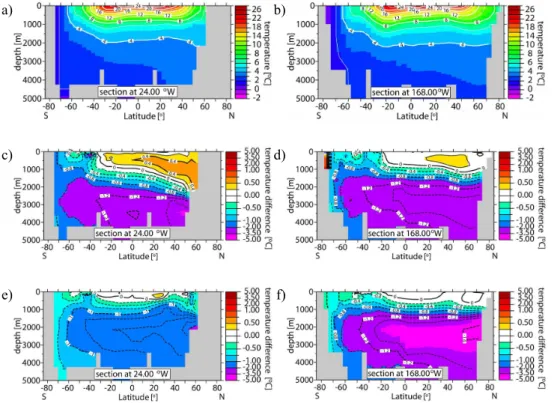
Figure 2 shows temperature sections along 25◦_{W and 170}◦_{W, i.e., in the Atlantic} Ocean and Pacific Ocean, respectively at 20 Ma. Figure 3 depicts the same for 14 Ma.

25

The upper panels show temperature in the control runs, whereas the middle and bottom panels show temperature differences relative to the control experiments.

(7)

CPD

6, 2687–2701, 2010

Title Page

Tables Figures

◭ ◮

Back Close

Full Screen / Esc

Discussion

P

a

per

|

Dis

cussion

P

a

per

|

Discussion

P

a

per

|

Discussio

n

P

a

per

of 40◦_{S at 14 Ma than at 20 Ma. The increased northward oceanic heat transport and} increased deepwater formation does lead to a slightly stronger pumping of warmer wa-ter into the deep ocean in the Northern Hemisphere (NH) at 20 Ma (Fig. 2c and d). However, there is no significant increase in deepwater formation in the NH contradict-ing a simple bi-polar seesaw scheme at 14 Ma. Where the bi-polar scheme is valid, a

5

significant, significant drop of deepwater production in the Southern Hemisphere (SH) from 85 Sv to 55 Sv in the 14 Ma hosing experiment (Exp. m14-2, Table 1) would have led to noteceably strongr nothbound overturning. Therefore, we argue that ocean-land geometry has precident over the other controls, including freshwater, of deepwater formation in high latitudes.

10

The amplitude and duration of the freshwater impacts are identical in both sets of experiments and the background atmospheric boundary conditions are very similar as well. Yet the response of the deep ocean to a southern freshening impact is noticeably different. Commonly to both sets, the expected warming of the deep ocean did not happen. Warming occurs mostly in the upper ocean in the NH and in the southern

15

tropics. In fact, this warming of the upper ocean occurs coincidently with cooling of the deep ocean. It is not yet clear what might have caused such counter-intuitive behavior. Salinizing of proto SO water around Antarctica increases during the early Miocene (Exp. m20-3). Surprisingly, the meridional overturning south of 40◦_{S and the} merid-ional overturning north of 40◦_{N decreases despite of salinizing. Consequently, the} 20

“heat piracy” (“stealing” heat from the opposite hemisphere) decreases from−1.5 PW to−1.53 PW (Table 1) (1 PW=1015W). Salinizing in the SH does not seem to have any sizable effect. This outcome supports the idea of lower SST, rather than higher SSS, being a primary control of the southern overturning. In contrast, freshening can hamper the overturning even if temperature remains close to freezing point. Meridional

25

temperature sections in both the Atlantic and Pacific do not change noticeably in the deep ocean (Fig. 2e and f).

(8)

CPD

6, 2687–2701, 2010

Title Page

Tables Figures

◭ ◮

Back Close

Full Screen / Esc

Discussion

P

a

per

|

Dis

cussion

P

a

per

|

Discussion

P

a

per

|

Discussio

n

P

a

per

|

Counter-intuitively, the meridional overturning south of 40◦_{S slows from 85 Sv to 65 Sv} and the oceanic cross-equatorial heat transport decreases from−1.3 PW to−0.8 PW.

In some studies it has been suggested (see the discussion and more references in Wright and Miller, 1996), that during the warm climates of the Mesozoic and early Cenozoic a poleward flow of warm saline deepwater (WSDW) originated in the low

lati-5

tudes ascending in high southern latitudes. None of our experiments show a formation of WSDW in low latitudes. In all runs, for Miocene 20 and 14 Ma, with and without fresh-water disturbances (salinizing or freshening), deepfresh-water always formed in the high and never in the low latitudes. Even in more distant past, the Early Cretaceous, a relatively warm deep ocean can exist with deepwater formed in the high latitudes in one of the

10

hemispheres (Haupt and Seidov, 2001); see also (Brady et al., 1998).

3 Discussion and conclusions

We hope that our results shed some new light on whether ocean changes might have accompanied the fluctuation of the sea ice extends of the young Antarctic Ice Sheet in the Miocene. The numerical experiments indicate higher sensitivity of the Miocene

15

ocean circulation to freshwater hosing in the proto Southern Ocean then of the present-day climate. One possible explanation is that it is the opening of the Central American Isthmus that was responsible for a stronger than present-day sensitivity of the ocean thermohaline circulation to small freshwater disturbances in the SO around Antarctica. Model 20 and 14 Ma configurations differ only in ocean-land geometry, yet the overall

20

ocean’s response to exactly the same freshwater impacts is very different. Thus it is a plausible assumption that the geometry of the proto-ACC which is responsible for these differences. Moreover, we argue that relatively small and geologically short-lived changes in freshwater balance in the SO could be responsible, at least partially, for at least two prominent disruptions of the dynamic Miocene’s general cooling trend.

25

(9)

CPD

6, 2687–2701, 2010

Title Page

Tables Figures

◭ ◮

Back Close

Full Screen / Esc

Discussion

P

a

per

|

Dis

cussion

P

a

per

|

Discussion

P

a

per

|

Discussio

n

P

a

per

Acknowledgements. This study was partly supported by NSF (NSF projects # 0224605 and ATM 00-00545).

References

Aagaard, K., Fahrbach, E., Meincke, J., and Swift, J. H.: Saline outflow from the Arctic Ocean: Its contribution to the deep waters of the Greenland, Norwegian, and Iceland seas, J.

Geo-5

phys. Res., 96, 20433–20441, 1991.

Abreu, V. S. and Anderson, J. B.: Glacial eustacy during the Cenozoic: Sequence stratigraphic implications, American Association Petroleum Geologists Bulletin, 82, 1385–1400, 1998. Barron, E. J. and Peterson, W. H.: The Cenozoic ocean circulation based on ocean general

circulation model results, Palaeogeogr. Palaeocl., 83, 1–28, 1991.

10

Barron, E. J. and Moore, G. T.: Climate model applications in paleoenvironmental analysis, SEPM Short Course Notes, Geological Society Publishing, Tulsa, Oklahoma, USA, 339 pp., 1994.

Bice, K. L., Scotese, C. R., Seidov, D., and Barron, E. J.: Quantifying the role of geographic change in Cenozoic ocean heat transport using uncoupled atmosphere and ocean models,

15

Palaeogeogr. Palaeocl., 161, 295–310, 2000.

Brady, E. C., DeConto, R. M., and Thompson, S. L.: Deep water formation and poleward ocean heat transport in the warm climate extreme of the Cretaceous (80 Ma), Geophys. Res. Lett., 25, 4205–4208, 1998.

Bush, A. B. G. and Philander, S. G. H.: The late Cretaceous: Simulation with a coupled

20

atmosphere-ocean general circulation model, Paleoceanography, 12, 495–516, 1997. Cox, M. and Bryan, K.: A numerical model of the ventilated thermocline, J. Phys. Oceanogr.,

14, 674–687, 1984.

Crowley, T. J. and North, G. R.: Paleoclimatology, New York, Oxford Univ. Press, 339 pp., 1991. Dickens, J. M.: Ocean-atmosphere feedback in climate simulations using off-line modules of a

25

coupled ocean-atmosphere model, Department of Meteorology, Pennsylvania State Univer-sity, University Park, 77 pp., 2004.

(10)

CPD

6, 2687–2701, 2010

Title Page

Tables Figures

◭ ◮

Back Close

Full Screen / Esc

Discussion

P

a

per

|

Dis

cussion

P

a

per

|

Discussion

P

a

per

|

Discussio

n

P

a

per

|

Haupt, B. J. and Seidov, D.: Warm deep-water ocean conveyor during the Cretaceous time, Geology, 29, 295–298, 2001.

Haupt, B. J. and Seidov, D.: Strengths and weaknesses of the global ocean conveyor: Inter-basin freshwater disparities as the major control, Prog. Oceanogr., 73, 358–369, 2007. Herrmann, A. D.: Late Ordovician ocean-climate system and paleobiogeography, Pennsylvania

5

State University, University Park, PA, USA, 196 pp., 2003.

Herrmann, A. D., Haupt, B. J., Patzkowsky, M. E., Seidov, D., and Slingerland, R. L.: Response of Late Ordovician paleoceanography to changes in sea level, continental drift, and atmo-sphericpCO₂: potential causes for long-term cooling and glaciation, Palaeogeogr. Palaeocl., 210, 385–401, 2004.

10

Kluzek, E. B., Olson, J., Rosinski, J. M., Truesdale, J. E., and Vertenstein, M.: User’s Guide to NCAR CCM3.6, National Center for Atmospheric Research, Boulder, Colorado, 151 pp., 1999.

Maier-Reimer, E., Mikolajewicz, U., and Crowley, T.: Ocean general circulation model sensitivity experiment with an open central American isthmus, Paleoceanography, 5, 349–366, 1990.

15

Miller, K. G., Kominz, M. A., Browning, J. V., Wright, J. D., Mountain, G. S., Katz, M. E., Sug-arman, P. J., Cramer, B. S., Christie-Blick, N., and Pekar, S. F.: The Phanerozoic record of global sea-level change, Science, 310, 1293–1298, 2005.

Pacanowski, R. C.: MOM 2. Documentation, User’s Guide and Reference Manual, GFDL Ocean Technical Report #3.2, edited by: Pacanowski, R. C., Geophysical Fluid Dynamics

20

Laboratory/NOAA, Princeton, NJ, 329 pp., 1996.

Pagani, M., Zachos, J. C., Freeman, K. H., Tipple, B., and Bohaty, S.: Marked decline in atmospheric carbon dioxide concentrations during the Paleogene, Science, 309, 600–603, 2005.

Scotese, C. R.: Paleogeographic Atlas, PALEOMAP Progress Report 90-0497, University of

25

Texas at Arlington, Arlington, Texas, 37 pp., 1997.

Scotese, C. R., Ross, M. I., and Schettino, A.: Plate tectonic reconstruction and animation, EOS, 79, p. 334, 1998.

Seidov, D. G.: Auto-oscillations in the system ’large-scale circulation and synoptic ocean ed-dies, Izvestiya USSR Acad. Sc., Atmospheric and Oceanic Physics, 22, 679–685, 1986.

30

Seidov, D. and Haupt, B. J.: Global ocean thermohaline conveyor at present and in the late Quaternary, Geophys. Res. Lett., 24, 2817–2820, 1997.

(11)

CPD

6, 2687–2701, 2010

Title Page

Tables Figures

◭ ◮

Back Close

Full Screen / Esc

Discussion

P

a

per

|

Dis

cussion

P

a

per

|

Discussion

P

a

per

|

Discussio

n

P

a

per

Planet. Change, 36, 99–116, 2003a.

Seidov, D. and Haupt, B. J.: Freshwater teleconnections and ocean thermohaline circulation, Geophys. Res. Lett., 30, 1–4, 2003b.

Seidov, D. and Haupt, B. J.: How to run a minimalist’s global ocean conveyor, Geophys. Res. Lett., 32, 1–4, 2005.

5

Shellito, C. J., Sloan, L. C., and Huber, M.: Climate model sensitivity to atmospheric CO₂levels in the Early-Middle Paleogene, Palaeogeogr. Palaeocl., 193, 113–123, 2003.

Stouffer, R. J., Seidov, D., and Haupt, B. J.: Climate Response to external sources of freshwa-ter: North Atlantic versus the Southern Ocean, J. Climate, 20, 436–448, 2007.

Thomas, E.: Descent into the icehouse, Geology, 36, 191–192, 10.1130/focus022008.1, 2008.

10

Toggweiler, J. R. and Bjornsson, H.: Drake Passage and palaeoclimate, J. Quaternary. Sci., 15, 319–328, 2000.

Vertenstein, M. and Kluzek, E. B.: User’s Guide to LSM1.1, National Center for Atmospheric Research, Boulder, Colorado, 26, 1999.

Wright, J. D. and Miller, K. G.: Control of the North Atlantic Deep Water circulation by the

15

Greenland-Scotland ridge, Paleoceanography, 11, 157–170, 1996.

Zachos, J. C., Dickens, G. R., and Zeebe, R. E.: An early Cenozoic perspective on greenhouse warming and carbon-cycle dynamics, Nature, 451, 279–283, doi:210.1038/nature06588, 2008.

(12)

CPD

6, 2687–2701, 2010

Title Page

Tables Figures

◭ ◮

Back Close

Full Screen / Esc

Discussion

P

a

per

|

Dis

cussion

P

a

per

|

Discussion

P

a

per

|

Discussio

n

P

a

per

|

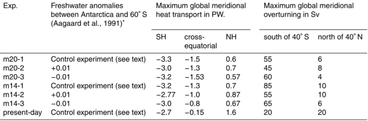
Table 1.Freshwater fluxes between the coast Antarctica and 60◦_{S. (}∗_{Added/removed water is}

redistributed over the entire sea surface to conserve water and salt balance in the World Ocean. Plus means added freshwater (hosing; fresher surface water), and minus means removal of freshwater (saltier surface water). The rates are in Sv; m20 stands for early Miocene (∼20 Ma)

and m14 for middle Miocene (∼14 Ma)).

Exp. Freshwater anomalies Maximum global meridional Maximum global meridional

between Antarctica and 60◦_S _{heat transport in PW.} _{overturning in Sv}

(Aagaard et al., 1991)∗

SH cross- NH south of 40◦_S _{north of 40}◦_N

equatorial

m20-1 Control experiment (see text) −3.3 −1.5 0.6 55 6

m20-2 +0.01 −3.0 −1.3 0.7 45 8

m20-3 −0.01 −3.2 −1.53 0.57 60 4

m14-1 Control experiment (see text) −3.2 −1.3 0.7 85 10

m14-2 +0.01 −2.77 −1.0 0.87 55 10

m14-3 −0.01 −3.0 −0.8 0.67 65 6

(13)

CPD

6, 2687–2701, 2010

Title Page

Tables Figures

◭ ◮

Back Close

Full Screen / Esc

Discussion

P

a

per

|

Dis

cussion

P

a

per

|

Discussion

P

a

per

|

Discussio

n

P

a

per

a)

b)

(14)

CPD

6, 2687–2701, 2010

Title Page

Tables Figures

◭ ◮

Back Close

Full Screen / Esc

Discussion

P

a

per

|

Dis

cussion

P

a

per

|

Discussion

P

a

per

|

Discussio

n

P

a

per

|

a) b)

c) d)

e) f)

Fig. 2.Temperature sections in the Atlantic (left column) and Pacific Oceans (right column):(a)

(15)

CPD

6, 2687–2701, 2010

Title Page

Tables Figures

◭ ◮

Back Close

Full Screen / Esc

Discussion

P

a

per

|

Dis

cussion

P

a

per

|

Discussion

P

a

per

|

Discussio

n

P

a

per

a) b)

c) d)

e) f)

Fig. 3. As in Fig. 2 for 14 Ma. Temperature sections in the Atlantic (left column) and Pacific

Oceans (right column): (a)and(b)Exp. m14-1,(c)and(d)Exp. m14-2 minus m14-1,(e)and