Abstract—The identification problem of periodically varying systems is considered in this paper. It is demonstrated that the systems with periodically varying parameters can be estimated using orthogonal functions; in this case the model can be approximated by Hartley series in the continuous range. The main advantage of using orthogonal functions is that the integro-differential equations are transformed into algebraic equations, this facilitates the identification process. The method presented in this paper was used to estimate parameters in the main rotor model of a helicopter, with satisfactory results.
Index Terms— System identification, periodically varying parameters, Hartley series, basis function, operational matrix.
I. INTRODUCTION
In a wide variety of practical applications, the characteristics of the plant dynamics are changing through time due to aging of components or the variation of the reference. When the dynamics of the system is changing at a slow pace, the least squares algorithm (with and without forgetting factor) is quite effective when it is used to follow this type of behavior. Nevertheless, the efficiency of the algorithm diminishes when the dynamics is changing rapidly. In the past years, systems with fast changing dynamics are being used more often in modern engineering applications; in particular, linear periodic time varying systems (LPTVS) have appeared in different areas such as Control, Power Electronics, Aeronautics, Communications and Signal Processing [1]. For example, in aeronautics, the equations that describe the flight dynamics in aircrafts have coefficients that are functions of time. Recently, the high speeds and accelerations that modern aircrafts can handle, have contributed to show that the parameters of the system that depend on speed will change in the same fashion. For instance, the dynamic of a main rotor in a helicopter, which can be modeled by a linear periodic system, is important from the control perspective due to the fact that a precise control of certain variables in the system can help to attenuate vibrations in the rotor components, that eventually may cause high levels of stress and fatigue [2]. Thus, there
Manuscript received July 23, 2012; revised August 9, 2012.
Isidro I. Lázaro is with the Electrical Engineering Department of the Universidad Michoacana de San Nicolás de Hidalgo, Morelia, México. (mail: [email protected]).
Alberto Álvarez is a graduate student at the Electrical Engineering Department of the Universidad Michoacana de San Nicolás de Hidalgo, Morelia, México. (mail: [email protected]).
Juan Anzurez is with the Electrical Engineering Department of the Universidad Michoacana de San Nicolás de Hidalgo, Morelia, México. (mail: [email protected]).
are important reasons to develop parametric identification techniques for this type of systems, some of these methodologies can be found in [3]-[5]. Also, the use of basis functions and operational matrices allows the approximation of system parameters of a previously known model; therefore, the LPTVS can be estimated through an approximation using orthogonal series [6]-[10].
The use of orthogonal series expansions is well known as an alternative for approximation and representation of functions. During the last two decades, algebraic methods have been established for the solution of problems described by differential equations, such as analysis of linear time invariant and time varying systems, model reduction, optimal control and system identification. The problem of parameter identification using orthogonal series includes linear time varying/invariant systems, lumped and distributed systems, also the nonlinear case.
The main purpose of this paper is to provide an alternative method for parametric identification. It is based on the transformation of the integro-differential equations that are used to describe the system into an algebraic set of equations. Some other advantages of this methodology are: easy implementation of the algorithm in computational packages (Matlab, Mathematica, C code, etc.) and the easy control of the identification procedure and its algorithm.
The structure of this paper is as follows: Section 2 is dedicated to the general background on approximation using Hartley series expansions and operational matrices. In section 3, the algorithm for the parametric identification for linear periodically time varying systems is presented. The application of the presented method and the associated results can be found in Section 4. The last section is devoted to the conclusions of this work.
II. ORTHOGONAL SERIES EXPANSIONS AND OPERATIONAL
PROPIERTIES VIA HARTLEY SERIES
In this section a brief review of the Hartley series is given. It can be stated that the kernel function of the familiar Fourier transform and Fourier series is complex exponential,
!!!"#.
The Hartley transform and series uses a similar frequency based kernel, the function cos !" +sin (!"), also known as the cosine and sine function or !"#(∙) [11].
Ident
ification
of
Linear
Periodically
Time
-Varying Systems
B
ased on
Hartley
Series
A. Hartley Series
An integrable function f(t) defined over the interval (0,!)
can be approximated in terms of Hartley series as f t F
( )
tt Φ = ) ( (1) Where
F=
[
F−n F−1 F0 F1 Fn]
(1,2n+1) (2)
[
]
tn n
t) φ φ1 φ0 φ1 φ
( = − −
Φ (3)
The basis functions for the Hartley series can be defined
as !!=!"# !"# =cos !"# +sin (!"#).
Each coefficient of the vector F, is calculated as follows
∫
Φ
=
t
n
k
f
t
t
dt
F
0
)
(
)
(
(4)Therefore, every function that complies with the Dirichlet conditions in the interval (0,!) can be approximated by means of a matrix product, as indicated by (1). The number of terms in the series is related to the error level; in this case, more terms mean a better approximation and a reduction in the error. The operational properties of the orthogonal series can be written in terms of an integration matrix, where the main idea is the fact that the integral of an orthogonal series can be expressed also as an orthogonal series; in general, this property can be defined as
(
)
(
)
0 0t
P
d
T
n t n t nΦ
=
∫
∫
τ
τ
(5)In the case of the Hartley series, the structure of the
integration matrix P is presented in [8] and it is shown in the
following equation
P=!1
!1 n 1 n ! " !1 2 1 2
!1 1
1
n
1
2 1
! !1 !1
2
1
n
!1 1 !1 2 1 2 ! " !1 n 1 n " # $ $ $ $ $ $ $ $ $ $ $ $ $ $ $ $ $ $ $ % & ' ' ' ' ' ' ' ' ' ' ' ' ' ' ' ' ' ' '
(2n+1)((2n+1)
(6)
For the analysis of LPTV Systems, two additional matrices must be defined, the product matrix and the coefficient matrix. The product of the vector of basis functions and its transpose gives the product matrix, this is
( )
t( ) ( )
t
t
t
Π
=
Φ
Φ
(7)The coefficient matrix is defined in terms of the product matrix and the vector of basis functions. This matrix satisfies the following relation
[ ]
C Φ( )t = ( )∏t c (8)The matrix C, of order 2n+1 is the coefficient matrix
when a vector c is given.
[ ]
0 1 1 2 2 3 2 2 1 1
1 1 1 1
1 1 0 2 1 1
3 3 3 3
1 1 1 1
2 2 0 1 2 2 2 2
3 3 3 3
3 2 1 0 1 2 3
1 1 0 1
2 2 2 2 1
3 3 2 2
2 2 0
2 2 0
2 2
1
2 2 2 2 2 2 2
2
2 2
c c c c c c c c c c
c c c c
c c c c c c
c c c c
c c c c
c c c c c c c c
c c c c
C c c c c c c c
c c c c c
c c c c c
c c c c
− − − − − − − − − − − − − − − − − − − − − − − − − − − − − + + − + + − + − + − + + + − + + + − + + = − + − + + + + − 1 2 2 2 2
1 1 1 1
1 1 2 0 1 1
3 3 3 3
1 1 2 2 3 2 2 1 1 0
0 2 2
0 2 2
c c
c c
c c c c
c c c c c c
c c c c
c c c c c c c c c c
− − − − − − − − − − − − ⎡ ⎤ ⎢ ⎥ ⎢ ⎥ ⎢ ⎥ ⎢ ⎥ ⎢ ⎥ ⎢ ⎥ ⎢ ⎥ ⎢ ⎥ ⎢ ⎥ ⎢ ⎥ ⎢ ⎥ ⎢ ⎥ ⎢ ⎥ + ⎢ + − ⎥ ⎢ ⎥ − + ⎢ ⎥ + + ⎢ ⎥ + + + − ⎢ ⎥ ⎢ ⎥ − + + + ⎢ ⎥ ⎢ ⎥ ⎣ ⎦ (9)
III. PARAMETER ESTIMATION FOR LINEAR PERIODICALLY TIME-VARYING SYSTEMS
Any given differential equation of degree n can be expressed as a set of state-space equations. This same set can be transformed into an algebraic set of equations using operational matrices. In this section, a methodology to solve the identification problem and estimate the unknown parameters using the input-output data is presented [12].
A. Identification Algorithm
Linear periodically time-varying systems can be described in general sense by the following set of state-space equations
( )
( ) ( )
( ) ( )
•
t = t t + t t
x A x B u (10)
where !(!)∈ℜ!×!
and !(!)∈ℜ!×! are the state and
input vectors respectively, and !(!)∈ℜ!×!
and !(!)∈ ℜ!×! are the corresponding periodic coefficients with the following properties
( )
t =(
t+T for)
0≤ ≤t TA A B
( )
t =B(
t+T for)
0≤ ≤t T (11)Using function approximations via orthogonal series, the expressions for the elements aij(t) and bij(t) of matrices A(t) and B(t) that satisfy the Dirichlet conditions in the interval
(0,!), can be expressed as
'
( ) ( )
ij ij
a t ≅AΦ t
b t
ij( )
≅
B
ij'Φ
( )
t
(12) WhereAij'
= A
!n A0 An
"
# $% Bij
'
= B
!n B0 Bn
"
# $%
(13) Similarly, the elements of vector !(!)∈ℜ!"!
and
'
( )
( )
i i
x t
≅
X
Φ
t
'( ) ( )
i i
u t ≅UΦt
(14)
With this in mind, the orthogonal series of the product
A(t)x(t) is
A(t)x(t)=
A11 '!
(t)X1 '!
(t)++A
1n '!
(t)X n '!
(t)
A21 '!(
t)X1 '!
(t)++A
2n ' !
(t)X n '!
(t) !
A
n1 '!
(t)X
1 '!
(t)++A
nn ' !
(t)X n '!
(t) "
# $ $ $ $ $ $
%
& ' ' ' ' ' '
(15)
Where every factor !!"! ! ! !!!!(!) may be rearranged using the product and coefficient matrix as follows
' ' ' '
( ) ( ) ( ) ( ) ( ) ( )
ij j ij j ij j
AΦt X tΦt =AΦ Φt t X =A ⎣⎡X ⎦⎤Φ t (16)
Matrix [!!]∈ℜ(
!×!) is the coefficient matrix of the vector !(!)∈ℜ!"!
where m =2n+1. It may be shown that with the above simplification, the product ! ! !(!) may be written as
A(t)x(t)=
A11 '
A12
' A
1n
'
A
21
' A
22
' A
2n
'
! ! " !
A
n1
' A
n2
' A
nn
'
!
" # # # # # #
$
% & & & & & &
X1
!" #$
X2
!" #$
!
X n
!" #$ !
" % % % % % %
#
$ & & & & & &
'(t)
(17) In other words,
A t x t( ) ( )=A X
[ ]
Φ( )t (18)Where [!!] is the coefficient matrix corresponding to
each coefficient, ! is the matrix formed by all the coefficient matrices [!!].A is the matrix formed for every
vector [!′!"] and Φ(!) is the basis vector. A similar procedure is used for B(t)u(t) yielding
[ ]
( ) ( ) B U ( )
B t u t = Φt
(19)
Where !(!)∈ℜ!×!(!), !(!)∈ℜ!(!×!) and
Φ(!)∈ℜ(!×!)
Integrating in both sides (10), we have that
0
0 0
( )
( )
( ) ( )
( ) ( )
t t
x t
−
x
t
=
∫
A t x t dt
+
∫
B t u t dt
(20)Using operational matrices and substituting (18) and (19) into (20) yields
[ ]
[ ]
0
( ) ( ) A X ( ) B U ( )
XΦt =XΦt + PΦt + Φ P t
(21) Where X0is the same size of X and contains the initial conditions of every state.
X0=
0 x
1(0) 0
! ! ! ! !
0 x
n(0) 0
!
" # # # #
$
% & & & &
(22)
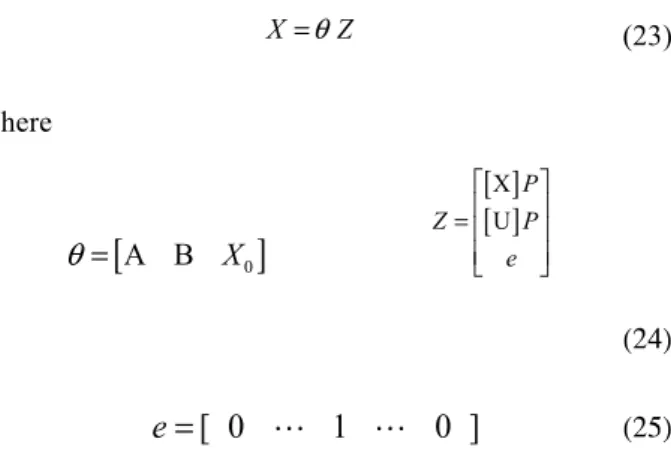
Equation (21) can be rewritten as
X=θ Z
(23) Where
[
A B X0]
θ
=[ ]
[ ]
X UP
Z P
e
⎡ ⎤
⎢ ⎥
=⎢ ⎥
⎢ ⎥
⎣ ⎦
(24)
e
=
[ 0
1
0 ]
(25)Using the above equations and solving for the unknown parameters we obtain [9]:
' ' 1 ( )
XZ ZZ
θ
−= (26) From the equation (26) the parameter coefficients can be obtained provided that (!!!)!! exists.
B. Analytical Redundancy
In dynamic systems, it is common to find physical redundancy, for example in the implementation of several devices of the same characteristics within the same measurement and control system. Another example consists in the use two or more sensors to anticipate every eventuality before a failure that causes system instability occurs. Another alternative, that is often more economical, is the application of analytical redundancy. This kind of redundancy involves the ability to run multiple experiments on the system to identify; the use of more than one input enables the excitation of the different operation modes in the
system for every experiment. Another option is to apply the
same signal at different frequencies and change the phase or/and magnitude. Subsequently, all this information is used for parameter estimation, as shown in Fig. 1. The disadvantage of this method is the off-line identification.
Fig. 1. Analytical redundancy scheme.
IV. APPLICATIONS
A simple theoretical second order periodic system is used as an introductory example in order to illustrate the methodology described in section III. Then, the application of the procedure is shown using the equations of the dynamics of a helicopter main rotor in forward flight.
System
System
System
Excitation u1
Excitation u2
Excitation uk
Output y2 Output y1
Output yk
Measuring states
Inputs
A. Second Order Periodic System
Let´s consider a second order linear system with a periodic coefficient described by [13].
( )
•
1
0 1 0
( ) ( )
1 1
t x t u t f
⎡ ⎤ ⎡ ⎤
=⎢ ⎥ +⎢ ⎥
− − ⎣ ⎦
⎣ ⎦
x
(27)
Where f1is a system with periodically varying parameters given by
f1(t)=1+sin(5
!t
) (28)And excited by a periodic input u(t)=sign
(
(sin!t))
and ω=2π.In order to perform the parametric identification of the system described by (27), equation (26) was used considering only the first 15 terms of the Hartley series and an analytical redundancy of 3. The system was excited off-line, with the purpose of having simulation data corresponding to the input-output behavior, with the following signals
u
1
(
t
)
=
sign
(
(sin
!
t
)
)
u
2(t)=1.2cos(3!t)+0.5cos(5!t)
u
3(t)=1+0.2cos(3!t)+0.05cos(5!t)
(29)
The simulation results obtained with the help of Matlab are shown in Fig. 2. In this figure, the parametric
identification of matrix A(t) is displayed when using only 15
terms of the Hartley series and it can be seen the difference between the estimated and real values. Fig 3. Shows the
results for the constant coefficients of matrix B(t)
Fig. 2. Parameter estimates of A(t) with n = 15.
Fig. 3. Parameter estimates of B(t) with n = 15.
With the purpose of improving the approximation between the estimated and the real parameter values, another test was performed considering 35 terms of the Hartley series. Fig. 4. Shows the improvements of the identification for the only periodic time-varying parameter in the system
a22(t). In this case, the varying nature of the parameters is
sinusoidal; therefore, the use of Hartley series for parametric identification is adequate since a low number of terms are
used in the estimation process.
Fig. 4. Parameter estimate a22(t) with n = 35.
B. Helicopter Main Rotor Model
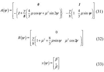
The equations that describe the dynamics in frontal flight of a helicopter main rotor are presented in [14]-[15]. The model for one of the blades can be written in the form of a linear periodic system, and has the following form
( )
( ) ( )
( ) ( )
•
ψ = ψ ψ + ψ ψ
x A x B u
(30)
Each matrix in (30) is described by 0 0.5 1 1.5 2
-3 -2 -1 0
1 a11 vs a11 estimated
Time (seconds)
0 0.5 1 1.5 2 0
0.5 1 1.5
2 a12 vs a12 estimated
Time (seconds)
0 0.5 1 1.5 2 -6
-4 -2 0 2
a21 vs a21 estimated
Time (seconds)
0 0.5 1 1.5 2 -4
-3 -2 -1 0 1
a22 vs a22 estimated
Time (seconds)
0 0.2 0.4 0.6 0.8 1 1.2 1.4 1.6 1.8 2
-0.1 -0.05 0 0.05
0.1 b11 vs b11 estimated
Time (seconds)
0 0.2 0.4 0.6 0.8 1 1.2 1.4 1.6 1.8 2
0.7 0.8 0.9 1 1.1 1.2
b21 vs b21 estimated
Time (seconds)
0.2 0.4 0.6 0.8 1 1.2 1.4 1.6 1.8 -6
-5 -4 -3 -2 -1 0 1 2 3
4 a22 vs a22 estimated
( )
4 2 4cos sin 2 1 sin
3 8 3
ψ γ γ
µ ψ µ ψ µ ψ
⎡ ⎤
⎢ ⎧ ⎫ ⎥
⎛ ⎞ ⎛ ⎞
⎢ ⎨ ⎜ + ⎟⎬ − ⎜ +⎟⎥
⎢ ⎩ ⎝ ⎠⎭ ⎝ ⎠⎥
⎣ ⎦
0 1
A = - 1 +
8
(31)
( )
2 20
8
1 sin cos 2
8 3
Bψ γ
µ µ ψ µ ψ
⎡ ⎤
⎢ ⎥
⎛ ⎞
⎢ ⎜ + + − ⎟⎥
⎢ ⎝ ⎠⎥
⎣ ⎦
= (32)
( )
xβ ψ
β• ⎡ ⎤ ⎢ ⎥ ⎢ ⎥ ⎣ ⎦
= (33)
Where µ=0.3 represents the advance ratio of the helicopter and γ =8 is the Lock number. In this case, ψ=ωt , and ω is the angular velocity. The first state variable β represents the angle of the blade with respect to the rotation plane and it is shown in Fig. 5.
Fig. 5. Main rotor simplified diagram.
In order to illustrate the identification procedure of LPTV systems, the aforementioned rotor model is used (30). The analytical redundancy value used in the simulation was 4, and the off-line applied signals that were used to obtain input-output measurements were
1( ) 1 0.1cos(5 )
u t = + t
2( ) 0.8cos(2 ) 0.1cos(5 )
u t = t + t
3
( )
3
0.1sin(3 )
u
t
=
t
+
t
4( ) 1.1cos( ) 0.2sin(3 ) 0.15cos(3 ) 0.1sin(5 )
u t = t + t + t + t
(34)
A total of 35 terms of the Hartley Series were used to perform the identification procedure. Four different signals
are used to generate the set of measurements (state x(t) and
input u(t)) when the analytical redundancy value is 4.
Applying the concepts of operational matrices, the [X] and [U] coefficient matrices are generated and employed in the off-line identification technique.
The algorithms to identify the periodic parameters in the model were developed in Matlab and the results obtained from comparing the estimated vs. real parameters of matrix
A(t) can be seen in Fig. 6 and 7 when n = 15. A small error
can be observed and it is even smaller for the second cycle of operation in the system. The error tends to decrease when
the value of n increases.
Fig. 6. Parameter estimates of A(t) with n = 15.
Fig. 7. Parameter estimates of B(t) with n = 15.
Figures 8 and 9 show the estimated parameters for
matrices A(t) and B(t) when n = 35. Again, the correlation
between the real values and the estimated ones, for both invariant and periodically variant parameters, can be seen.
In Fig. 10, the absolute error of the periodic parameters in
matrix A(t) is displayed. From this graphic, it can be seen
that the error between estimated and real values decreases drastically after the transitory effect of the identification test and when the number of terms used in the Hartley series increases.
0 5 10 -2.5
-2 -1.5 -1 -0.5 0 0.5
a11 vs a11 estimated
Time (periods)
0 5 10 0.5
1 1.5 2 2.5
a12 vs a12 estimated
Time (periods)
0 5 10 -2.5
-2 -1.5 -1 -0.5 0
a21 vs a21 estimated
Time (periods)
0 5 10 -2
-1 0 1
a22 vs a22 estimated
Time (periods)
0 2 4 6 8 10 12
-0.4 -0.2 0 0.2
0.4 b11 vs b11 estimated
Time (periods)
0 2 4 6 8 10 12
0 0.5 1 1.5 2
2.5 b21 vs b21 estimated
Fig. 8. Parameter estimates of A(t) with n = 35.
Fig. 9. Parameter estimates of A(t) with n = 35.
Fig. 10. Absolute error of A21(t) and A22(t) with n = 35.
It is worth mentioning that not necessarily all the terms in the orthogonal series that are used in the identification process have great significance. For instance, the estimated
parameter a22(t) has only 15 terms that are significant; the
values of the rest of the terms are less than 10% of the Hartley series coefficient of higher magnitude. Therefore, to
estimate the parameter, only an expansion in orthogonal series of 15 out of 35 terms is needed.
V. CONCLUSIONS
A frequency domain technique for off-line parameter estimation of LPTV systems has been presented. The operational matrices tools and the integration matrix in particular, are used to yield algebraic equations that allow the parameter identification procedure to take place. These algebraic equations can be solved through the use of a pseudoinverse. The presented procedure is applied to two different cases using Hartley series as the basis function. These properties are used to estimate the parameters of a second order theoretical system with only one time-varying parameter, and also of the model that describes the dynamics of the main rotor of a helicopter in forward flight.
From the comparison made between the estimated and real parameters, for both cases, it can be seen that the average error decreases when the number of terms used in the series is increased. It is also important to notice that the number of terms to be considered in the estimation process can be reduced if only the parameters with higher
magnitudes are taken into account.
REFERENCES
[1] H. Zhao, J. Bentsman, “Wavelet-based Identification of Fast Linear
Time-Varying Systems Using Function Space Methods,” in 2000
Proc.of the American Control Conference, pp. 939-934.
[2] R. Pandiyan and S. C. Sinha, “Periodic Flap Control of a Helicopter
Blade in Forward Flight”, Journal of Vibration and Control, vol. 5,
pp. 761–777, 1999.
[3] M. Niedzwiecki, An Identification of Time-varying Processes. New
York: John Wiley & Sons, Ltd, 2000.
[4] T. Bohlin, Four cases of identification of changing systems. In
Systems Identification: Advances and Cases Studies, New York: Academic Press, 1987.
[5] L. Ljung and T. Sodrstrom, Theory and Practice of Recursive
Identification. The MIT Press, Upper Saddle River, N.J. 1983.
[6] K. B. Datta, B. M. Mohan, “Orthogonal Functions in Systems and
Control”,Singapore: World Scientific vol 9. 1995.
[7] Z. Qizhi,L. Li, “Identification of Time-Varying System Based Fourier
Series,” in 2009 Global Congress on Intelligent Systems, pp. 44-47.
[8] A. Baños, F. Gómez, “Parametric identification of transfer funtions
from frequency response data,” Computing & Control Engineering
journal, pp. 137-144, June 1995.
[9] S. D. Fassois, D. E. Rivera, “Applications of System Identification,”
IEEE Control Systems Magazine, Vol. 27-5,pp. 24-26, October 2007,.
[10] C. Y. Yang, C. K. Chen, “Analysis and Optimal Control of
Time-Varying Systems via Fourier,” International Journal of Systems
Science, Vol.25, No.11,pp. 1663-1678, 1994
[11] J. J. Rico, G. T. Heydt, A. Keyhani, B. L. Agrawal, D. Selin,
“Synchronous machine parameter estimation Using the Hartley
series,” IEEE Trans. on Energy Conversion, vol.16, pp. 49-54, Mar.
2001.
[12] D. Alejo, I. Lázaro, J. Rico, A. Álvarez, “Parameter estimation of
linear and nonlinear systems based orthogonal series,” in Procedia
Engineering. International Meeting of Electrical Engineering Research ENIINVIE, Ensenada México, 2012, pp. 67–76.
[13] J. A. Álvarez, J. Rico, J. J. Rincón, “Exact steady state analysis in
power converters using floquet decomposition”, North American Power Symposium (NAPS), Boston, USA, 2011.
[14] C. Shoulz, “Rotorcraft smoothing via linear time periodic methods”,
Ph.D. dissertation, Air Force Institute of Technology, United State of America, 2007.
[15] J. A. Álvarez, “Herramientas de modelado matemático de sistemas
periódicos aplicados al cálculo del estado estable y al diseño de controladores,” M.S. thesis, Dept. Electrical. Eng., UMSNH. Morelia, México, 2012.
0 5 10 -2.5
-2 -1.5 -1 -0.5 0
0.5 a11 vs a11 estimated
Time (periods)
0 5 10 0.5
1 1.5 2
2.5 a12 vs a12 estimated
Time (periods)
0 5 10 -2.5
-2 -1.5 -1 -0.5
0 a21 vs a21 estimated
Time (periods)
0 5 10 -2
-1 0
1 a22 vs a22 estimated
Time (periods)
0 2 4 6 8 10 12
-0.4 -0.2 0 0.2
0.4 b11 vs b11 estimated
Time (periods)
0 2 4 6 8 10 12
0 0.5 1 1.5 2
2.5 b21 vs b21 estimated
Time (periods)
0 2 4 6 8 10 12
0 0.5 1 1.5 2 2.5
Time (periods)
Ab
s
o
lu
te
e
rr
o
r
Parameter A21
0 2 4 6 8 10 12
0 0.5 1 1.5 2 2.5
Time (periods)
Ab
s
o
lu
te
e
rr
o
r