www.atmos-chem-phys.net/15/12361/2015/ doi:10.5194/acp-15-12361-2015
© Author(s) 2015. CC Attribution 3.0 License.
Spatial and temporal variability of clouds and precipitation over
Germany: multiscale simulations across the “gray zone”
C. Barthlott and C. Hoose
Institute of Meteorology and Climate Research (IMK-TRO), Karlsruhe Institute of Technology (KIT), Karlsruhe, Germany
Correspondence to:C. Barthlott ([email protected])
Received: 26 May 2015 – Published in Atmos. Chem. Phys. Discuss.: 24 June 2015 Revised: 16 September 2015 – Accepted: 2 November 2015 – Published: 9 November 2015
Abstract.This paper assesses the resolution dependance of clouds and precipitation over Germany by numerical sim-ulations with the COnsortium for Small-scale MOdeling (COSMO) model. Six intensive observation periods of the HOPE (HD(CP)2Observational Prototype Experiment) mea-surement campaign conducted in spring 2013 and 1 sum-mer day of the same year are simulated. By means of a se-ries of grid-refinement resolution tests (horizontal grid spac-ing 2.8, 1 km, 500, and 250 m), the applicability of the COSMO model to represent real weather events in the gray zone, i.e., the scale ranging between the mesoscale limit (no turbulence resolved) and the large-eddy simulation limit (energy-containing turbulence resolved), is tested. To the au-thors’ knowledge, this paper presents the first non-idealized COSMO simulations in the peer-reviewed literature at the 250–500 m scale. It is found that the kinetic energy spectra derived from model output show the expected−5/3 slope, as well as a dependency on model resolution, and that the effec-tive resolution lies between 6 and 7 times the nominal reso-lution. Although the representation of a number of processes is enhanced with resolution (e.g., boundary-layer thermals, low-level convergence zones, gravity waves), their influence on the temporal evolution of precipitation is rather weak. However, rain intensities vary with resolution, leading to dif-ferences in the total rain amount of up to +48 %. Further-more, the location of rain is similar for the springtime cases with moderate and strong synoptic forcing, whereas signifi-cant differences are obtained for the summertime case with air mass convection. Domain-averaged liquid water paths and cloud condensate profiles are used to analyze the tem-poral and spatial variability of the simulated clouds. Finally, probability density functions of convection-related parame-ters are analyzed to investigate their dependance on model
resolution and their impact on cloud formation and subse-quent precipitation.
1 Introduction
The quantitative forecast of precipitation and clouds is still a challenge for state-of-the-art numerical models on both short-range weather time scales and climate time scales. Al-though the phenomena responsible for triggering convection are broadly known (Jorgensen and Weckwerth, 2003; Ben-nett et al., 2006), the forecasting skill especially for heavy convective showers is still low. A large part of the inac-curacy results from the difficulties of the models to initi-ate cloud formation and convective processes at the right place and time (e.g., Barthlott et al., 2011). Besides uncertain initial and boundary conditions, inaccuracies of numerical methods and/or the incomplete description of physical pro-cesses influence the performance of the numerical models. The successful simulation of convection initiation over land, which is strongly forced from the surface, depends on hav-ing a reasonable representation of boundary-layer processes and the development of shallow cumulus convection (e.g., Petch et al., 2002). Some of the boundary-layer circulations, such as convective rolls, drylines, gust fronts, orographic cir-culations, and circulations resulting from mesoscale surface heterogeneities (i.e., land use, soil moisture), are precursors of cloud formation and convective development (Jorgensen and Weckwerth, 2003).
started (http://hdcp2.eu). HD(CP)2 is a Germany-wide ini-tiative funded by the Federal Ministry of Education and Re-search (BMBF). Besides the development of a new model system capable of conducting very-high-resolution simula-tions over domains of 1000 km, a fundamental part of the project was a large measurement campaign entitled HOPE (HD(CP)2Observational Prototype Experiment). HOPE was conducted in spring 2013 near Jülich in western Germany and included a large variety of in situ and remote sensing in-struments. Based on these measurements, the model can be evaluated critically on the scale of the model simulations and information is obtained on subgrid-scale variability and mi-crophysical properties that are subject to parameterizations. A major observation system operated during HOPE was the so-called KITcube (Kalthoff et al., 2013), which is a monitor-ing system consistmonitor-ing of different in situ and remote sensmonitor-ing instruments.
In smaller-scale meteorological applications, two classes of numerical modeling are distinguished: mesoscale mod-eling on larger domains and large-eddy simulations (LES) on the smaller ones (Wyngaard, 2004). The ratio of the energy-containing turbulence scale and the scale of the spa-tial filter used in the equations of motion l/1is small for mesoscale modeling (no turbulence resolved) and large for LES (energy-containing turbulence is resolved). With in-creasing computer power in the last years, it is now possi-ble to conduct very finely meshed simulations withl/1∼1. Since neither LES nor mesoscale models were designed to operate in this range, it was called “terra incognita” or “gray zone” (Wyngaard, 2004). For the HD(CP)2 project, it was decided to jump over this gray zone with the development of a new model system ICON (ICOsahedral Non-hydrostatic; Zängl et al., 2015) which can be operated for domains with 1000 km×1000 km at a horizontal grid spacing of 100 m. Since current operational models still operate in this range (e.g., German Weather Service: 2.8 km; UK Met Office: 1.5 km; Meteo France: 2.5 km), it is of interest to understand which results can be obtained from simulations within the gray zone in order to assess the impact of grid spacing on quantitative precipitation forecasting.
In recent years, many studies were devoted to exploring the resolution dependance of numerical weather forecasting for different synoptic conditions and geographical areas. The most remarkable feature of numerical models with grid spac-ing smaller than 2–4 km is the possibility to explicitly treat deep convection instead of using a parameterization. Many studies have shown that such models provide quantitatively better results in terms of the simulated precipitation amount, its structure, and timing (e.g., Done et al., 2004; Weisman et al., 2008; Bauer et al., 2011). However, small-scale up-drafts and the turbulent nature of the flow can only be repre-sented adequately by large-eddy simulations at a grid length of 100 m or less (Bryan et al., 2003). Thus, the convection-permitting models operating at the order O(1 km) have major
shortcomings in regards to the nature of convective clouds (Hanley et al., 2014).
Once convection-permitting resolutions are reached, it re-mains unclear as to whether increasingly fine horizontal grid spacing alone can result in further increases in forecast skill (e.g., Roebber et al., 2004). Recent findings of Kain et al. (2008) and Schwartz et al. (2009) suggest that decreasing horizontal grid spacing from 4 to 1–2 km provides little added value and that forecast skill in the USA is not im-proved. One possible reason may be that more sophisticated physical parameterizations (e.g., for boundary-layer turbu-lence or cloud microphysics) are needed at such high res-olution. However, there are also opposite findings of refin-ing the mesh size havrefin-ing improved the quantitative precip-itation forecast results: for example, Zängl (2007) investi-gated two north-Alpine heavy-rainfall cases with a variable number of nested domains, resulting in finest mesh sizes of 9, 3, and 1 km. The runs with high grid resolutions had a highly beneficial impact in the Alpine part of the area due to a proper representation of the topography. For a case study of a quasi-stationary convective system over the UK South-west Peninsula, Warren et al. (2014) found several deficien-cies in the 1.5 km model’s representation of the storm sys-tem. However, significant improvements regarding convec-tion initiaconvec-tion were found when the grid length was reduced to 500 m due to an improved representation of a convergence line. Hanley et al. (2014) simulated several convective events over the southern UK at horizontal grid lengths ranging from 1.5 km to 200 m with the Met Office Unified Model. Their results suggest that convection is under-resolved at a grid length of 1.5 km. Although an improvement in convection initiation time was observed when reducing the grid length, the size and intensity of the cells were not necessarily proved. Furthermore, changing the mixing length often im-proves one aspect of the simulated convection, while another aspect is affected adversely.
repre-sentation of the diurnal cycle of convective organization over West Africa by a 4 km model compared to a 12 km configu-ration was a result of the convection scheme rather than the improved resolution.
Whereas most of the above-mentioned studies of resolu-tion dependance of numerical weather forecasting with real-istic model configurations were conducted at or above the or-der O(1 km), only a few studies are available for grid lengths ranging between 100 m and 1 km: e.g., Boutle et al. (2014) for a case of stratocumulus evolution or Green and Zhang (2015) for a modeling study of Hurricane Katrina. Most of the studies in this range used idealized configurations (e.g., Bryan et al., 2003; Wyngaard, 2004; Fiori et al., 2009, 2011; Verrelle et al., 2015). These previous studies suggest that hor-izontal resolution may be important when modeling cloud formation and precipitation. However, it remains unclear whether the model features originally designed for the sim-ulation of larger-scale atmospheric flows will yield adequate reproductions of small-scale motions (Gibbs and Fedorovich, 2014). This line of investigation is now extended by nu-merical simulations of realistic cases with quasi-operational model settings but different model resolutions. As cloud evo-lution and turbulence still need to be parameterized on that scale, a good representation of subgrid-scale variability is es-sential. Therefore, the focus of this paper lies not only on the impact of a higher grid spacing on cloud and precipitation development but also on the variability of convection and cloud-related parameters and how this variability changes with model resolution. Instead of analyzing mean values of such parameters, probability distributions show the range of possible values and the most probable ones. To this end, we systematically explore the gray zone and test the applicabil-ity of the COnsortium for Small-scale MOdeling (COSMO) model at high resolutions to several cases with different syn-optic conditions.
2 Method
In order to investigate the potential benefits of a higher grid resolution for the simulation of convective rain, a series of numerical simulations were performed using version 5.0 of the COSMO model. This section describes the model config-uration and the days chosen for this study.
2.1 Numerical model
The COSMO model is a non-hydrostatic regional weather forecast model (Schättler et al., 2013) used for opera-tional weather forecasting at the Deutscher Wetterdienst (DWD, German Weather Service) and several other Euro-pean weather services. It employs an Arakawa C-grid for horizontal differencing on a rotated latitude/longitude grid. To minimize problems resulting from the convergence of the meridians, the pole of the grid is rotated such that the
equa-tor runs through the center of the model domain. In the ver-tical direction, a terrain-following, hybrid height coordinate is used. A two-time level Runge–Kutta method (Wicker and Skamarock, 2002) for time integration is implemented. The microphysics scheme includes riming processes (graupel for-mation) and predicts cloud water, rain water, cloud ice, snow, and graupel. A multi-layer soil vegetation model (TERRA-ML; Doms et al., 2011) is implemented.
At the DWD, the application COSMO-EU of the COSMO model provides operational forecasts for all of Europe at 7 km grid spacing with initial and boundary conditions de-rived from the hydrostatic global model GME (mesh size 40 km). Deep and shallow convection are parameterized us-ing a Tiedtke scheme (Tiedtke, 1989) in COSMO-EU. In ad-dition, a convection-permitting version (COSMO-DE) with 2.8 km grid spacing is used for Germany and smaller parts of neighboring countries. The horizontal grid spacing of 2.8 km allows the parameterization of deep convection to be switched off. Small-scale shallow convection is parameter-ized using a modified Tiedtke scheme. According to Baldauf et al. (2011), the operational COSMO-DE produces satisfac-tory results in synoptically driven situations, but the model (as many other operational models, too) still has problems correctly describing convection initiation at the right time and place in air mass convection situations.
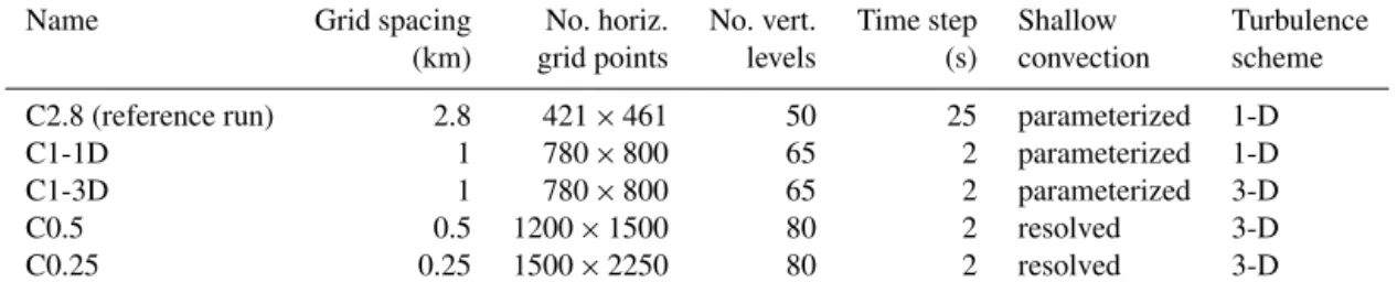
In this study, numerical simulations with horizontal grid spacings of 2.8 km, 1 km, 500 m, and 250 m have been con-ducted (Table 1). The run with 2.8 km resolution corresponds to the operational setup used by the DWD and serves as the reference run in this study. Note that also the number of ver-tical levels is increased for the 1 km runs and the 500/250 m runs. This limits somehow the conclusions of this study, be-cause the results are affected by both horizontal and verti-cal grid spacing. However, when moving to finer-resolution simulations, it is also meaningful to increase the number of vertical levels. In doing so, especially the representation of processes in the planetary boundary layer (PBL) and the en-trainment zone is supposed to be enhanced. The number of levels in the lowest 1000 m is 12, 15, and 18 for the runs with 50, 65, and 80 levels, respectively.
Table 1.Model configuration details.
Name Grid spacing No. horiz. No. vert. Time step Shallow Turbulence
(km) grid points levels (s) convection scheme
C2.8 (reference run) 2.8 421×461 50 25 parameterized 1-D
C1-1D 1 780×800 65 2 parameterized 1-D
C1-3D 1 780×800 65 2 parameterized 3-D
C0.5 0.5 1200×1500 80 2 resolved 3-D
C0.25 0.25 1500×2250 80 2 resolved 3-D
this scale, while the formulation used in LES may not be ap-propriate. Therefore, the 1 km model was run with both a 1-D and a 3-D turbulence scheme. For the finer resolutions of 500 and 250 m, only the 3-D turbulence scheme was applied. For the 500 and 250 m runs, the parameterization of shallow con-vection is switched off whereas the runs with coarser resolu-tion still need this parameterizaresolu-tion to be active to adequately simulate the moisture transport from the surface to the cloud layer (Tiedtke, 1989; Doms et al., 2011).
The 2.8 km runs used a time step of 25 s, whereas all other runs used a value of 2 s. This large reduction in the time step was necessary to prevent numerical problems and model instabilities over steep orography. COSMO-EU anal-yses serve as initial and boundary conditions for the refer-ence run, whose outcome is then used to drive all of the higher-resolution simulations. Since no suite of nesting is performed and the same driving data are used for the resolu-tion below 2.8 km, the interpretaresolu-tion of the numerical results is facilitated. In a sensitivity experiment (not shown), a suite of nested domains was used, but the results differed only marginally from those of the above configuration. The lat-eral boundary update interval is 1 h (2.8 km grid spacing) and 15 min for the remaining model runs. The smaller interval is due to the smaller model domain which makes it necessary to prevent showers (or large-scale phenomena) persisting for a long time at the edges of the model domain. All model runs do not include data assimilation or feedbacks between indi-vidual nests. Each model run is initialized at 00:00 UTC with an integration time of 24 h.
The simulation domain (Fig. 1) of the reference run is identical to the COSMO-DE operational configuration. It is aimed at using the largest possible domain for the high-resolution simulations, but numerical problems for very steep orography and the required data storage capacities and com-puting time lead to smaller simulation domains as model res-olution increases. For the analysis presented later, a common domain was chosen to be somewhat smaller than the 250 m run to prevent edge effects (black rectangle in Fig. 1).
An important feature of our simulations is the fact that we use the same external data (orography, soil type, land use) for all model runs. The external data are based on 30 arcsec (1 km) gridded, quality-controlled Global Land One-km Base Elevation Project (GLOBE) orography, the
Figure 1.Simulation domains. The dashed rectangle indicates the
common investigation area used in this study. The measurement area of the HOPE field campaign is located around the KITcube position.
Global Land Cover 2000 Project (GLC 2000) for a harmo-nized land cover, and the Food and Agriculture Organization of the United Nations (FAO) Digital Soil Map of the World (DSMW). This data set was interpolated on the respective model grids with an internal consistency check. This means that all changes in the simulation results are a response to a different model resolution only and are not linked to a bet-ter representation of the underlying orography and land data. The model orography in the 2.8 km configuration smoothes out some of the orographic features (like smaller valleys) vis-ible at 1 km resolution and also maximum elevations of indi-vidual mountain ridges are lower compared to the 1 km data (not shown). When interpolating to the 500 and 250 m grids, the orographic features of the 1 km data stay the same, with the exception of minor interpolation artifacts at the coastline.
2.2 Cases analyzed
Table 2.Weather characteristics at the HOPE measurement site for the intensive observation periods (IOP) used in this study. “n/a” means not applicable.
Day (IOP) Weather characteristics
15 April (IOP 3)
broken cumulus cloudiness in the morning, overcast during noon (11:00–16:00 UTC) with light rain, clearance in the evening, weak wind
24 April (IOP 6)
clear-sky day with only few cirrus clouds in the morning and afternoon, weak southerly winds
25 April (IOP 7)
cloudy morning (up to 4/8) until 10:00 UTC, only a few clouds during noon, afterwards again increasing cumulus humilis cloudiness, wind turns from south to west in the afternoon
26 April (IOP 8)
rapidly increasing cloudiness up to complete overcast situation until noon, several rain showers and light to medium rain, decreasing cloudiness in the late afternoon, quickly turning wind from south to north during midday due to front passage, decreasing temperatures
19 May (IOP 14)
fog in the morning, afterwards clear-sky conditions until late afternoon, only very few low cumulus humilis clouds, rising cirrus clouds in the afternoon to evening, wind from north
28 May (IOP 18)
clear-sky conditions until midday (10:00 UTC) with only very few cirrus clouds, following low cumulus humilis clouds until 17:00 UTC, afterwards rapidly increasing cloudiness with rain starting in the evening, wind turns from south to east
23 July (n/a)
decaying convective showers during night, afterwards clear-sky conditions, after 12:00 UTC widespread initiation of deep convection
type of event, simulations were performed for a summer case with air mass convection (see Table 2).
For the description of the synoptic situation of the selected days, we use theQvector at 500 hPa:
Q= −R p
∂v
g
∂x · ∇T , ∂vg
∂y · ∇T
, (1)
whereR is the gas constant of dry air, p is pressure,vg is
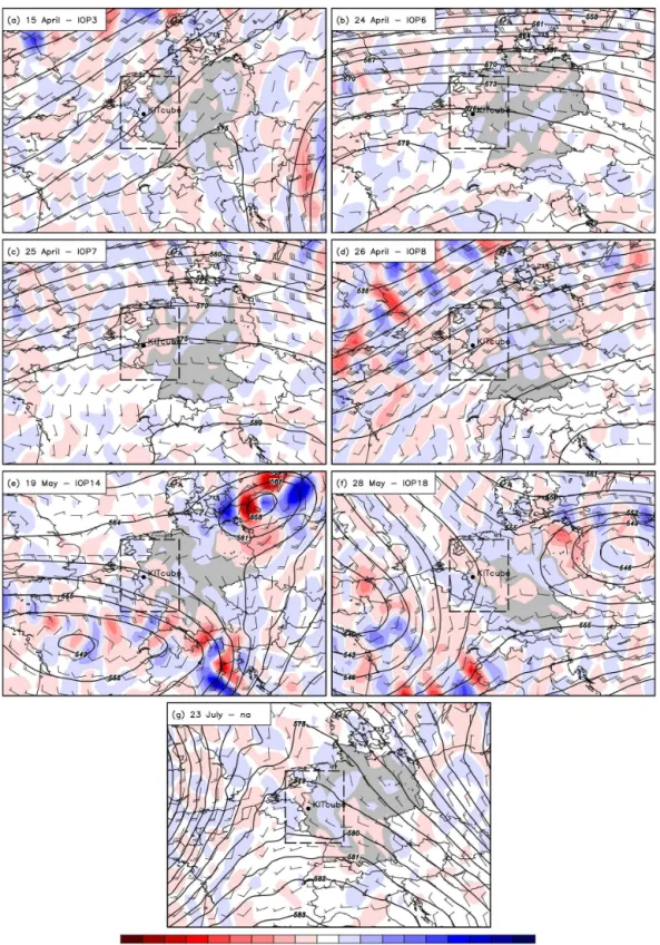
the geostrophic wind, andT is temperature (Hoskins et al., 1978). Areas with forcing for upward (downward) vertical motion are associated with Q vector convergence (diver-gence). In our study, the Qvector is estimated from 7 km COSMO-EU analyses which also serve as initial and bound-ary condition for our simulations. Figure 2 shows the synop-tic conditions of the selected days at 12:00 UTC. On 15 April (Fig. 2a), a weak southwesterly flow is present with only weakQvector convergence. A ridge over southeastern Ger-many inhibits convective processes in that area. Over western and northwestern Germany, however, radar-derived measure-ments show widespread moderate amounts of rain with up to 10–15 mm (Fig. 3a). The conditions on 24 and 25 April (Fig. 2b and c) are similar: a moderate westerly flow to-gether with only small forcing for upward and downward motion. On both days, no precipitation is measured near the KITcube location. Only small amounts of rain are observed in the northern part of the investigation area on 25 April (Fig. 3b). The mid-tropospheric flow intensifies on the next day (26 April, Fig. 2d) with the flow direction turning to southwest. On this day, radar measurements indicate
pre-cipitation almost over entire Germany with 24 h accumu-lations of up to 30 mm (Fig. 3c). The maximum, but still small, rain amounts are observed to the north and south of the KITcube location. On 19 May (Fig. 2e), two low-pressure regions influence Germany, one of them being located north of Poland and the other over central France. The HOPE mea-surement site is located at the northern edge of the low over France with weak easterly winds. In the southern part of Germany, spatially widespread precipitation is observed with peaks of 90 mm, whereas the measurement site is free of rain (Fig. 3d). A long-wave trough extending from Iceland towards northwestern France leads to a southerly flow on 28 May (Fig. 2f). There are convective showers over south-ern Germany and eastsouth-ern France as well as moderate rain over the HOPE domain (Fig. 3e). The last day of the cases analyzed (23 July, Fig. 2g) shows a strong ridge over west-ern Germany and eastwest-ern France. Despite the convection-inhibiting effect of subsidence, several isolated convective showers are initiated in that area (Fig. 3f).
3 Model results
Figure 2. COSMO-EU analyses for 12:00 UTC showing 500 hPa geopotential height (gpdm, contours), Q vector divergence
(10−17m(kg s)−1, shading), and horizontal wind (knots). Red colors indicate forcing for upward motion and blue colors for downward
Figure 3.Precipitation amount over 24 h, derived from radar mea-surements (interpolated to the operational COSMO-DE model grid with 2.8 km horizontal grid spacing) for the analyzed days. The area shown is the common investigation area already depicted in Fig. 1. Note that 24 April is not shown due to the lack of observed precipi-tation.
3.1 Benefits of high-resolution modeling for gravity waves, low-level wind convergence, and PBL thermals
In this section, the benefits of high-resolution modeling in simulating atmospheric processes is demonstrated by the analysis of gravity waves, low-level convergence zones, and PBL thermals. As the results concerning these features are very similar in both 1 km runs (with either 1-D or 3-D
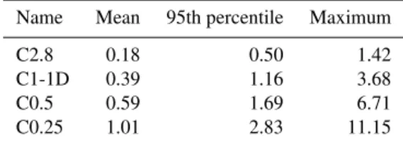
tur-Table 3. Characteristics of low-level wind convergence on
15 April 2013 at 16:00 UTC in 10−3s−1.
Name Mean 95th percentile Maximum
C2.8 0.18 0.50 1.42
C1-1D 0.39 1.16 3.68
C0.5 0.59 1.69 6.71
C0.25 1.01 2.83 11.15
bulence scheme), we only show the outcome of the run with 1-D scheme. Figure 4 presents a comparison of the simu-lated vertical velocities at 2.9 km a.s.l. for 26 April 2013 for the different horizontal grid spacings used. Obviously, the C2.8 run cannot resolve any gravity wave activity on that day. With a grid spacing of 1 km or below, however, gravity waves are simulated in the southern part of the investigation area. The location of the waves over the mountainous terrain indicates that these waves are induced by orographic lifting of air masses in the presence of stable temperature stratifi-cation. Although more fine-scale structures can be seen with even higher resolution (500, 250 m), the locations of the in-dividual regions with upward and downward vertical motion and, thus, the wavelength of the waves (ranging between 11 and 13 km) remains identical. The intensity of the vertical motions, however, increases slightly with model resolution. On this day, satellite pictures document the existence of grav-ity waves with similar wave lengths and extents in that area (not shown). Due to the fact that the locations of the waves are similar in the high-resolution runs and the intensity in-creases only slightly with model resolution, it can be stated that a horizontal grid spacing of 1 km should be sufficient for capturing the general characteristics of atmospheric gravity waves at least for the locations and meteorological conditions studied in this paper.
Figure 4.Vertical wind (color shading in m s−1at 2900 m a.s.l. on
26 April 2013 at 11:30 UTC for(a)2.8 km,(b)1 km with 1-D
tur-bulence,(c)500 m, and(d)250 m grid spacing. Gray shading
rep-resents model orography in m.
of the areas with the strongest convergence is rather insen-sitive to model resolution, since there are only minor spa-tial differences. Besides the increasing ratio of grid points with convergence, the mean value of convergence (only pos-itive contributions), the 95th percentile, and the maximum convergence do increase with grid spacing (Table 3). The increased convergence intensity has important implications for convection initiation due to reduced entrainment (e.g., Garcia-Carreras et al., 2011) and stronger lifting which may allow rising parcels to attain their level of free convection. It is also worth mentioning that there is an area almost free of convergence ranging from Köln towards Bremen. This zone is simulated in all model runs and is associated with a calm post-frontal region. With increasing grid spacing, however, this area is continuously reduced in size.
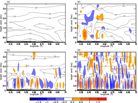
25 April is chosen to examine the evolution of boundary-layer thermals, because the region of interest is cloudless around noon. Figure 6 presents vertical cross sections of ver-tical wind and equivalent potential temperature at the latitude of the KITcube location during HOPE (see Fig. 1). Due to the coarse resolution of the 2.8 km run, no PBL thermals can
Figure 5. 10 m wind convergence (shading in 10−3s−1) on
15 April 2013 at 16:00 UTC for(a)2.8 km,(b)1 km with 1-D
tur-bulence,(c)500 m, and(d)250 m grid spacing.
Figure 6.Vertical cross sections of vertical wind speed (shading, in m s−1) and equivalent potential temperature (gray contours in◦C) at the
latitude of the KITcube location on 25 April 2013 at 12:00 UTC for(a)2.8 km,(b)1 km with 1-D turbulence,(c)500 m, and(d)250 m grid
spacing.
3.2 Effective model resolution
The previous section demonstrated that an increased model resolution leads to a better representation of a variety of me-teorological processes. To determine whether the parameter-izations used for the different model runs are valid at their applied resolution, we computed kinetic energy density spec-tra from model output in a similar way as proposed by Ska-marock (2004): at first, 1-D spectra of the three velocity com-ponents were computed along west–east horizontal grid lines in the entire common investigation area. The energy densi-ties were then averaged horizontally by averaging the west– east grid lines over the north–south extent of the area. Fi-nally, the energy densities were time averaged from 10:00 to 24:00 UTC (at 30 min intervals) to cover a statistically long enough time period. The late start time of 10:00 UTC was chosen to avoid model spin-up effects. This procedure was done for three heights (3, 5, and 7 km a.m.s.l.). As the results do not show any significant differences in terms of shape of the spectra, we show the result for 23 July 2013 in Fig. 7 at 5 km a.m.s.l. only. It can be seen that the am-plitude and wavelength of the energy spectra systematically vary with model resolution: similar to findings from Bryan et al. (2003), the magnitude increases with increasing model resolution and the spectra cover a wider (i.e., more small-scale) range of wavelengths. However, the high-frequency end of the spectra shows white noise only. For all model resolutions, the spectra show a region with a −5/3 decay in the mesoscale. This region reaches to higher wave
num-bers (shorter wavelengths) when model grid spacing is re-duced. The point where the gradients (in log space) of the individual spectra decrease below−5/3 determines the effec-tive resolution of the model. Previous studies have suggested that this occurs at length scales between 6 and 7 times the horizontal grid spacing (e.g., Bryan et al., 2003; Skamarock, 2004; Petrik, 2012). Our simulations show the same behav-ior; the gradient of the spectra decreases below −5/3 be-tween 6 and 71x(marked by the gray shaded areas). Another feature evident here is that the runs with 250 m grid spac-ing possess a region with slightly increased energy density (when compared to the−5/3 slope) before reaching the point of the effective resolution. This might be explained by en-ergy from shorter wavelengths aliased to longer wavelengths (Skamarock, 2004).
3.3 24 h precipitation amount
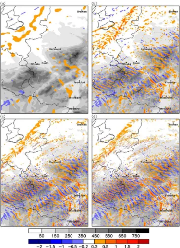
In this section, we analyze the 24 h accumulated precipita-tions of the numerical simulaprecipita-tions (Fig. 8) and compare them with radar-derived precipitation (Fig. 3). Since the focus of this paper is on investigating the resolution dependance of cloud and precipitation-related processes, a qualitative com-parison is made only and no quantitative verification methods are applied.
1 10
wavelength (km)
C2.8
~18.2
km
C1
~6.5
km
C0.5
~3.3
km
C0.25
~1.6
km
10-4 10-3 10-2
wavenumber (rad m-1)
1 10 102
103
E
(
k
)
(m
3/s 2)
C2.8 C1-1D C1-3D C0.5 C0.25
Figure 7.Kinetic energy density spectra computed from COSMO
model output for 23 July 2013 averaged between 10:00 and 18:00 UTC at a height of 5 km a.g.l. The gray shaded areas repre-sent wavelengths of 6–7 times the horizontal grid spacing of the
different model runs. Dashed lines with−5/3 slope are plotted to
aid identification of the inertial subrange.
differences in horizontal extent and precipitation amount are simulated: the C2.8 run has the smallest area covered by pre-cipitation of all model runs and the maximum rain amounts (15–20 mm) are simulated in the high-resolution runs with 3-D turbulence scheme (C1-33-D, C0.5, C0.25). A common error of all model realizations is the lack of more widespread pre-cipitation in the northwestern part when compared to radar observations (see Fig. 3a).
Due to the lack of observed and simulated precipitation, the 24 April case is not shown in Fig. 8. In the simulations for 25 April, a small west–east oriented area with precipitation is present somewhat north of and over the KITcube. Since only weak amounts of rain are simulated (less than 6 mm) and the precipitation location is nearly identical in all model runs, this case also is not shown in Fig. 8. The radar-derived observations, however, do not show any precipitation in that area.
The spatial rain distribution on 26 April (Fig. 8, second row) reveals that the entire investigation area is covered by rain. In all model runs, there is a band with highest rain amounts from the southwestern corner to the middle of the eastern edge of the domain. The structure of this band is more or less the same in all model runs. Whereas the max-ima (40–50 mm) agree well with radar observations, the area with strong rain amounts is too small (see Fig. 3c). The radar observations also show a region without rain west of the KITcube and another area with maximum rain amounts of 30–40 mm in the north, both of these features are not cap-tured by any of our model runs.
On 19 May, the simulations show widespread precipita-tion east and south of the KITcube (Fig. 8, third row). The
overall spatial distribution again is rather similar in all model runs, except for one convective cell east of Cologne (marked by a black circle). Whereas C2.8 and C1D (both with 1-D turbulence) simulate only moderate amounts of rain (6– 8 mm), all remaining runs simulate a small, but distinct, con-vective cell with precipitation accumulations of 30–40 mm (C1-3D) and even 40–50 mm (C0.5, C0.25). The higher grid spacing, together with the 3-D turbulence scheme, seems to create a more vigorous convective activity.
Several convective showers are simulated in the southern part of the investigation area (including the KITcube loca-tion) on 28 May (Fig. 8, fourth row). In that case, more dif-ferences in the spatial rain distribution between the individ-ual model runs can be observed. For example, the convec-tive cell marked by the black circle in the reference run C2.8 is not simulated by run C1-1D and only with reduced rain amount and shifted towards the south by the run C1-3D. With 500 and 250 m grid spacing, the cell is simulated again and the aggregation towards a convective line is visible. Another difference is the cloud-free region of the reference run east of the KITcube, which is also obvious from the radar observa-tion (Fig. 3e). In all other model realizaobserva-tions, however, there are several convective showers ranging up to the latitude of Dortmund. Even if the amounts of rain differ somewhat, the convective cells to the west of the KITcube are simulated similarly in all model runs.
Figure 8.Simulated 24 h accumulated precipitation in mm. Each row shows the results from 1 analyzed day for the different model runs. From top to bottom: 15, 26 April; 19, 28 May; 23 July 2013.
As 24 and 25 April show very small precipitation amounts only, these 2 days are excluded from the following analysis. For the remaining days, the simulated precipitation amount increases with model resolution (Fig. 9a), with the exception of 15 April, for which the C1-3D run simulates a slightly higher precipitation amount. However, the highest
radar-derived precipitation is higher than the simulated one on 15, 26 April, and 23 July, the opposite is true for 19 and 28 May. It is worth noting that either all runs reveal lower or higher precipitation amounts than derived by the radar. When neglecting 24 and 25 April again, the largest devia-tions from the reference run are found for the summer case of 23 July with an increase of 48 % by the 250 m run. On this day, this model run is also closest to the radar-derived precipitation amount, indicating an improved forecast qual-ity for the 24 h domain-accumulated precipitation amount at least. Other days exhibit also large deviations from the refer-ence run, e.g., 15 April (23–34 %). The percentage increase of the 24 h precipitation amount is lowest for 26 April and 19 May with maximum deviations from the reference run of 7 and 4 %, respectively. Those days also have the highest pre-cipitation accumulations of all analyzed days.
A more detailed look at the precipitation statistics is pro-vided by the box-and-whisker diagram in Fig. 9c. An impor-tant variable for hydrological processes and flash floods is the simulated maximum precipitation amount. Our results show that increasing the model resolution does not lead to sys-tematically increased maximum precipitation amounts. How-ever, with the exception of both 1 km runs for 26 April, the reference run with 2.8 km grid spacing always has the lowest maximum precipitation amount. Apart from that, large dif-ferences can occur, as can be seen, e.g., on 23 July, when the simulated maximum increases from 56 to 95 mm in 24 h. The median of the 24 h precipitation amount exhibits only small variations without any systematic response to model resolu-tion. Stronger variations can be seen for the 75 percentiles, particularly on 26 April. On that day, a comparatively small increase of domain-integrated precipitation is simulated with increased model resolution. As the 25 percentiles, the me-dian, and the simulated maximum precipitation amount show little variation only, the increase of the 75 percentiles seems to be responsible for the higher precipitation amount. When neglecting the days with small amounts of precipitation (15, 24, 25 April), the comparison with radar-derived observa-tions reveals that the median is rather well captured by the models on 19, 28 May, and on 23 July, whereas all model configurations have significantly lower median values on 26 April. The reference run on that day even exhibits a 75 percentile lower than the radar-derived median. This reflects the smaller precipitation amounts of the models when com-pared to the observations. There are also large differences concerning the maximum precipitation amount. While the difference on 26 April is comparably small, stronger devi-ations between observed and simulated maximum precipita-tion amounts are obvious on 19, 28 May, and 23 July.
3.4 Temporal evolution of precipitation
An important aspect of simulating precipitation is its tempo-ral evolution, i.e., the onset, duration, and end of convective precipitation. Although the initiation of individual convective
0 0.5 1.0 1.5 2.0
24
h
accumulated
precipitation
(10
12
l)
15 APR 26 APR 19 MAY 28 MAY 23 JULY IOP3 IOP8 IOP14 IOP18
radar-derived C2.8 C1-1D C1-3D C0.5 C0.25
(a)
0 10 20 30 40 50
deviation
from
C2.8
(%)
15 APR 26 APR 19 MAY 28 MAY 23 JULY IOP3 IOP8 IOP14 IOP18
C1-1D C1-3D C0.5 C0.25
(b)
0 10 20 30 40 50 60 70 80 90 100
24
h
precipitation
(mm)
radar-derived C2.8 C1-1D C1-3D C0.5 C0.25
15 APR 26 APR 19 MAY 28 MAY 23 JULY IOP3 IOP8 IOP14 IOP18
(c)
Figure 9.Domain-accumulated 24 h precipitation amount(a),
de-viation from reference run(b), and box-and-whisker diagram(c)
exhibiting the median, the 25 and 75 percentiles, as well as the
min-imum and maxmin-imum precipitation amounts. Note that in(c)only
grid points with precipitation larger than 0.5 mm are considered to prevent too small median values in case of small fractions of the area with convective precipitation.
0 2 4 6 8 10 12 14 16 18 20 22 24 time (UTC)
0 0.1 0.2
0.3 (e) 23 JULY
0 0.1
0.2 (d) 28 MAY - IOP18
0 0.2 0.4 0.6
mean
precipitation
(mm
30
min
-1)
(c) 19 MAY - IOP14 0
0.2 0.4
0.6 (b) 26 APR - IOP8 0
0.05 0.10 0.15
(a) 15 APR - IOP3
radar C2.8 C1-1D C1-3D C0.5 C0.25
Figure 10.Simulated and radar-derived mean precipitation rates of
the common investigation area.
As can be seen in Fig. 10, two dominating peaks of pre-cipitation at 11:00 and 16:30 UTC are observed by the radar on 15 April. Towards the end of that day, the mean itation rate increases again. The onset of simulated precip-itation in all model runs is only 30 min later than observed. Whereas the first dominating peak at 11:00 UTC is simulated at the same time, the second peak is simulated 1.5 h later. Furthermore, the simulated precipitation rates are consider-ably lower than the ones derived from radar measurements. All simulations show a similar mean precipitation rate until the time of the secondary precipitation peak. Later on, the C2.8 (C1-3D) run simulates the smallest (largest) precipita-tion rates of the individual model configuraprecipita-tions.
On 26 April, both simulated and radar-derived mean pre-cipitations start at the same time (04:00 UTC). After a strong increase, the observations show a broad maximum between 11:30 and 14:00 UTC. During that time, all simulations show precipitation rates that are half of the observations only. There is a gradual decrease in the observed precipita-tion rate to 0.2 mm 30 min−1. The simulations, however, re-veal another increase in convective activity with a peak at 18:30 UTC. This peak is slightly higher than the observed precipitation. The decrease of convective rain in the evening is simulated with values similar to those observed. Although all curves from the simulations are located close together, the runs with the 1-D turbulence (C2.8 and C1-1D) scheme
show slightly lower mean precipitation rates than the remain-ing model configurations.
After a first local maximum at 05:30 UTC, radar-derived precipitation on 19 May increases gradually up to its maxi-mum at 19:00 UTC. The models capture the onset and inten-sity of the mean precipitation rather well but the maximum rain intensity is simulated 1.5 h later than observed. Again, all models have similar rain intensities, with the 1-D turbu-lence scheme having slightly lower values.
On 28 May, observed and simulated precipitations start again at the same time (11:30 UTC). The maxima are sim-ulated at 16:30 UTC, which is only 30 min earlier than the observed peak. Later on, precipitation rates decrease but start to rise again after 21:00 UTC. Besides the higher maximum precipitation rates, the simulations show a rather good agree-ment with the observations on that day.
The air mass convection case of 23 July reveals some showers in the night and early morning (until 10:00 UTC). During that time, the models simulate only very little amounts of rain. After 11:00 UTC, simulated and observed precipitations increase simultaneously with similar values. Whereas the observations show a kind of plateau with more or less constant rain rates between 14:00 and 16:00 UTC, fol-lowed by a strong increase to its maximum at 18:00 UTC, the simulated rain rate maxima occur at different times between 13:30 and 16:30 UTC. Furthermore, all simulated peaks are somewhat lower than the one derived by radar. After their re-spective maximum, the mean rain intensities decrease again to almost 0 mm 30 min−1at 23:30 UTC.
grid spacing is stronger on days with weak synoptic-scale forcing and vice versa.
3.5 Characteristics of cloud liquid water path
To assess the influence of the model resolution on the sim-ulated clouds, we now analyze the cloud liquid water path (LWP; here as the sum of cloud water and rain water) of all days and all configurations. Figure 11 illustrates the time evolution of domain-averaged LWP and the fraction of grid points with LWP values exceeding 1 g m−2. In general, the temporal evolution of the domain-averaged LWP has a sim-ilar shape as the rain intensities displayed in Fig. 10. As ex-pected, the increase of the LWP always starts earlier than the respective rain increase. On days with predominantly con-vective showers (15 April, 28 May, and 23 July), the time delay is 1–2 h, whereas there is also a slowly increasing LWP on days with stronger large-scale forcing (26 April, 19 May) on which the first rain is simulated 4–5 h later. This difference in the time delay suggests that under con-vective situations forced by local processes, the growth of the clouds is faster than in situations with strong large-scale forcing, where a more gradual growth of the clouds (i.e., a slower transition from shallow to deep convection) is typi-cal. Non-precipitating clouds were simulated for the evening of 24 April. Only the C1-1D run simulates some clouds in the early morning, whereas the remaining runs do not. Fur-ther inspection of the cloud field revealed some isolated low clouds in that run, possibly due to a slightly colder PBL (not shown). The largest differences in mean LWP between the different model resolutions occur on 25 April, a day with only very small amounts of rain (less than 6 mm in 24 h). On that day, the runs with a 1-D turbulence scheme (C2.8, C1-1D) show noticeable higher mean values than the runs with the 3-D turbulence scheme, whereas the tempo-ral evolution is similar in all runs. Mean rain intensities, however, are rather similar with values between 0.05 and 0.07 mm 30 min−1. The fact that the runs with a 1-D turbu-lence scheme simulates larger LWP values is also true for 15 April (09:00–12:00 UTC) and 26 April (morning and af-ternoon). As can be seen from the fraction of grid points ex-ceeding 1 g m−2in the right column of Fig. 11, these periods are characterized by a larger cloud cover. As the maximum LWPs are very similar or even lower (not shown), we there-fore conclude that the larger mean LWP values are due to a larger fraction of grid points with simulated clouds than in the runs with a 3-D turbulence scheme. On the contrary, the area with simulated clouds is smaller in the runs with a 1-D turbulence scheme on 19 May for most of the day whereas the mean LWP is rather similar in all runs. This means that the lower rain amounts (despite similar rain intensities) in the runs C2.8 and C1-1D (see Fig. 9) can be attributed to some-what fewer clouds in the area of investigation. A possible ex-planation for the higher LWP in the runs with 1-D turbulence scheme for the aforementioned periods might be a stronger
entrainment of colder air from the free troposphere into the PBL. On 15 April at 10:00 UTC for example (not shown), the PBL is more than 1 K colder in the runs with a 1-D scheme. A shallow cloud layer between 800 and 1300 m a.g.l. is sim-ulated in those runs, whereas there are no clouds in the runs with a 3-D turbulence scheme. Although there is not much variation in the 24 h precipitation amount, our results show that the choice of the turbulence scheme can have a strong influence on PBL clouds.
3.6 Probability density functions and subgrid-scale variability of the reference run C2.8
In low-resolution models, clouds are parameterized based on assumptions regarding the subgrid-scale variability of ther-modynamic variables, with a prescribed probability density function (PDF) of fixed form and width being used (e.g., Tiedtke, 1989). The PDFs of cloud and convection-related variables, however, can vary significantly over space and time. To investigate the impact of higher grid spacing on cloud and precipitation development, we now analyze a num-ber of convection-related variables with their PDFs. Doing this, the variability of these parameters can be studied and it is found how the variability changes with model resolution. Analysis of PDFs also allows for the determination of the most probable values, which provides more insights into the atmospheric phenomena than analyzing mean or median val-ues. At first, we focus on PDFs calculated inside the common investigation area for the entire simulation period, meaning that every half-hourly model output over the entire simula-tion time of 24 h is taken into account (hereinafter referred to as 24 h PDF).
gen-0 2 4 6 8 10 12 14 16 18 20 22 24 time (UTC)
0 50 100 150
(m) 23JULY
0 2 4 6 8 10 12 14 16 18 20 22 24 time (UTC)
0 10 20
(n) 23JULY 0
20 40 60
80 (k) 28MAY - IOP18
0 10 20 30 40
50 (l) 28MAY - IOP18 0
100 200
(i) 19MAY - IOP14
mean
LWP
(g
m
-2)
0 20 40 60
80 (j) 19MAY - IOP14
area
fraction
LWP
>
1
g
m
-2
(%)
0 100
200 (g) 26APR - IOP8
0 20 40 60
80 (h) 26APR - IOP8 0
10 20 30 40
(e) 25APR - IOP7
0 10 20 30
40 (f) 25APR - IOP7 0
10
20 (c) 24APR - IOP6
0 10
20 (d) 24APR - IOP6 0
10
20 (a) 15APR - IOP3
C2.8 C1-1D C1-3D C0.5 C0.25
0 10 20
30 (b) 15APR - IOP3
Figure 11.Domain-averaged liquid water path (left column) and fraction of grid points with liquid water path values exceeding 1 g m−2
(right column) in the common investigation area.
eral dependance on the model resolution, however, is present on all days.
For continuity reasons, the convergence of the low-level wind must lead to the lifting of air parcels. Figure 12b shows the PDFs of vertical velocity in the PBL at a height of ∼
400 m a.g.l.As expected, the response of the PDFs to model resolution is identical to that of the low-level wind conver-gence: there are stronger up- and downdrafts at higher res-olutions with reduced probabilities of the dominant values. The analysis of PDFs of the vertical velocity at higher levels (850, 700, and 500 hPa) indicates that the systematic behav-ior observed in the PBL is persistent at all heights. Although their probabilities of occurrence are very low, the tails of the distribution become larger when reducing grid spacings.
The PBL characteristics and their impacts on the triggering and/or dynamics of convection depend on the partitioning of the available energy (net radiation minus ground heat flux) into sensible and latent heat, which in turn is determined by soil moisture. As the land use and soil type are identical in all runs, since they have been interpolated to a higher resolution, only small differences in the 24 h PDFs of the net radiation are observed (not shown), which is due to varying cloudiness or rain. Whereas the distributions of the latent heat flux are similar for all model resolutions, there are minor differences for the PDFs of the sensible heat flux (not shown). The high-resolution runs have a more pronounced peak with slightly
narrower PDFs compared to the runs at low resolution. These differences, however, occur for negative values simulated for stable, nighttime conditions only and are probably related to the 3-D turbulence scheme. The PDFs of the positive fluxes (from the ground to the atmosphere) are very similar for all model resolutions.
-0.004 -0.002 0 0.002 0.004
10 m wind convergence (s-1)
10-4 10-3 10-2 0.1
rel.
frequency
of
occurrence
C2.8 C1-1D C1-3D C0.5 C0.25 (a)
-1.2 -0.9 -0.6 -0.3 0 0.3 0.6 0.9 1.2
w 400 m agl (m s-1)
10-4 10-3 10-2 0.1
rel.
frequency
of
occurrence
C2.8 C1-1D C1-3D C0.5 C0.25 (b)
Figure 12.Probability density functions of the 10 m wind
conver-gence(a)and vertical velocity at∼400 m a.g.l.(b)on 23 July 2013.
do have their dominant value at slightly higher temperature on 23 July. The small differences in the PDFs of specific hu-midity and temperature can have strong impacts on the near-surface relative humidity. As can be seen in Fig. 13 (right), there are marked discrepancies between the dominant val-ues of the individual PDFs: on 25 April, the dominant value of the relative humidity is 53 % for runs C2.8 and C1-1D, whereas for the remaining runs, it is 85 %. For 23 July, there is even a systematic shift to higher values with increased model resolution. This tendency towards higher dominant values of relative humidity also is a feature of the other days under investigation. This has important implications for the evolution of PBL-driven convection. As was already pointed out by several authors (e.g., Crook, 1996), small variations in boundary-layer temperature and moisture (1◦C and 1 g kg−1,
respectively) can make the difference between no initiation and intense convection. Since our results reveal strong dif-ferences in the dominant values of near-surface relative hu-midity, this also affects the height of the lifting condensation level or the level of free convection. Especially for the July case with scattered convection, the implications of the differ-ences in the PDFs are reflected by the different precipitation structures (see Fig. 8). However, also on days with almost no
simulated precipitation (25 April, Fig. 13), the dominant val-ues of near-surface relative humidity can show strong varia-tions with model grid spacing. This indicates that the PDFs are modified not only by the different rain amounts and loca-tions as observed for the summertime case of 23 July but also by the pure response to model resolution without feedbacks from moist convection.
3.7 Temporal analysis of dominant values and variances
The previous section revealed the strong response of selected convection-related variables to model grid spacing based on PDFs for the entire 24 h simulation period. However, it is also of interest to analyze the temporal development of their characteristics. As the analysis of all parameters describing the distribution of variables, such as the variance, the mean, the median, the dominant, and extreme values, would require too large an expenditure, we focus our analysis in this sec-tion on the dominant values and the variances of the distri-butions. Figure 14 presents these characteristics for the 2 m temperature and 2 m specific humidity in steps of 30 min for the entire simulation domain of all days under investigation. The common color scale for all days somewhat limits the visibility of the variability of model runs for the individual days. Therefore, the deviations of these values from those of the reference run are also displayed in the right column. The temporal evolution of the dominant 2 m temperature shows a daily cycle linked to the warming of the near-surface air, with larger values around noon and in the afternoon. Max-ima of up to 33◦C are reached for the summertime case of
23 July. A significant drop of the dominant values from 17 to 8◦C occurs on 26 April between 13:30 and 14:00 UTC for all
model simulations of this day. The analysis of the individual PDFs of these times shows a bimodal distribution with local maxima at the above values. Although the overall shape of the PDF is similar, the dominant value shifts between these two values at 14:00 UTC. Inspection of the deviation from the dominant values of the reference run with 2.8 km grid spacing reveals strong differences of more than 5 K for the different model realizations at the same time. The reason for the bimodal distribution is the convective precipitation falling only in parts of the simulation domain: the PDFs of the 2 m temperature in the morning hours exhibit one promi-nent peak (not shown). In the course of the day, convective rain intensifies while progressing eastwards (see temporal evolution in Fig. 10). This leads to relatively warm temper-atures in the eastern part of the simulation domain, while the rain falling in the western parts leads to cooling. Con-sequently, a bimodal temperature distribution evolves with the change of the dominant value occurring at 14:00 UTC.
5 10 15 20 25 30 2 m temperature (° C)
0 0.01 0.02 0.03
rel.
frequency
of
occurrence
C2.8 C1-1D C1-3D C0.5 C0.25 (a)
15 20 25 30 35
2 m temperature (° C) 0
0.01 0.02
0.03 C2.8
C1-1D C1-3D C0.5 C0.25 (b)
4 6 8 10
2 m specific humidity (g kg-1) 0
0.02 0.04 0.06
rel.
frequency
of
occurrence
C2.8 C1-1D C1-3D C0.5 C0.25 (c)
6 8 10 12 14 16 18
2 m specific humidity (g kg-1) 0
0.01 0.02 0.03
C2.8 C1-1D C1-3D C0.5 C0.25 (d)
10 20 30 40 50 60 70 80 90 100 2 m relative humidity (%)
0 0.01 0.02
rel.
frequency
of
occurrence
C2.8 C1-1D C1-3D C0.5 C0.25
(e)
10 20 30 40 50 60 70 80 90 100 2 m relative humidity (%)
0 0.01 0.02 0.03
C2.8 C1-1D C1-3D C0.5 C0.25
(f)
Figure 13.Probability density functions of the 2 m temperature(a, b), 2 m specific humidity(c, d), and 2 m relative humidity(e, f)on
25 April (left) and 23 July 2013 (right).
warmer peak, whereas the remaining runs have their maxima at the colder one. As the model orography does only change from 2.8 to 1 km, these differences can be attributed to dif-ferent meteorological processes (slope winds, convergence, PBL processes in general) resulting from different model res-olutions only. The same holds for the negative deviation of the high-resolution runs on 23 July around 18:00 UTC.
Concerning the variance of the 2 m temperature, we find the highest values on days with the largest integrated rain amount (26 April, 19 May, 23 July). The individual maxima coincide with phases of larger dominant values. An important finding is the fact that the variance for a specific day does not necessarily increases with model resolution. Whereas a ten-dency of increased variance can be seen for most of the an-alyzed cases and times, there are three longer time periods on 25, 26 April, and on 19 May, where the 2 m temperature variance decreases with model resolution. Differences in
pre-cipitation intensity or amount cannot be responsible for this behavior, since the total rain amounts and timings of precip-itation for these phases are very similar in all model runs. We therefore suspect that besides the different horizontal and vertical grid spacings, the use of the 3-D turbulence scheme might play a role. Between 14:00 and 18:00 UTC on 23 July, the increase of the variance with resolution most probably is related to the later rain maximum simulated at high resolu-tions (see Fig. 10).
7 9 11 13 15 16 18 20 22 24 25 27 29 31 33
2 4 6 8 10 12 14 16 18 20 22 24 (a) T2m dominant value (° C)
15 APR 24 APR 25 APR 26 APR 19 MAY 28 MAY 23 JUL C2.8 C1-1D C1-3D C0.5 C0.25 C2.8 C1-1D C1-3D C0.5 C0.25 C2.8 C1-1D C1-3D C0.5 C0.25 C2.8 C1-1D C1-3D C0.5 C0.25 C2.8 C1-1D C1-3D C0.5 C0.25 C2.8 C1-1D C1-3D C0.5 C0.25 C2.8 C1-1D C1-3D C0.5 C0.25 -5.1 -4.4 -3.7 -2.9 -2.2 -1.5 -0.7 0 0.7 1.5 2.2 2.9 3.7 4.4 5.1
2 4 6 8 10 12 14 16 18 20 22 24 (b) T2m dominant value deviation from C2.8 (° C)
15 APR 24 APR 25 APR 26 APR 19 MAY 28 MAY 23 JUL C2.8 C1-1D C1-3D C0.5 C0.25 C2.8 C1-1D C1-3D C0.5 C0.25 C2.8 C1-1D C1-3D C0.5 C0.25 C2.8 C1-1D C1-3D C0.5 C0.25 C2.8 C1-1D C1-3D C0.5 C0.25 C2.8 C1-1D C1-3D C0.5 C0.25 C2.8 C1-1D C1-3D C0.5 C0.25 1 2 3 4 5 6 7 8 9 10 11 12 14 15 16
0 2 4 6 8 10 12 14 16 18 20 22 24 (c) T2m variance (° C)2
15 APR 24 APR 25 APR 26 APR 19 MAY 28 MAY 23 JUL C2.8 C1-1D C1-3D C0.5 C0.25 C2.8 C1-1D C1-3D C0.5 C0.25 C2.8 C1-1D C1-3D C0.5 C0.25 C2.8 C1-1D C1-3D C0.5 C0.25 C2.8 C1-1D C1-3D C0.5 C0.25 C2.8 C1-1D C1-3D C0.5 C0.25 C2.8 C1-1D C1-3D C0.5 C0.25 -3.3 -2.9 -2.4 -1.9 -1.4 -1.0 -0.5 0 0.5 1.0 1.4 1.9 2.4 2.9 3.3
0 2 4 6 8 10 12 14 16 18 20 22 24 (d) T2m variance deviation from C2.8 (° C)2
15 APR 24 APR 25 APR 26 APR 19 MAY 28 MAY 23 JUL C2.8 C1-1D C1-3D C0.5 C0.25 C2.8 C1-1D C1-3D C0.5 C0.25 C2.8 C1-1D C1-3D C0.5 C0.25 C2.8 C1-1D C1-3D C0.5 C0.25 C2.8 C1-1D C1-3D C0.5 C0.25 C2.8 C1-1D C1-3D C0.5 C0.25 C2.8 C1-1D C1-3D C0.5 C0.25 5.0 5.5 6.1 6.6 7.2 7.7 8.3 8.9 9.4 10.0 10.5 11.1 11.6 12.2 12.7
2 4 6 8 10 12 14 16 18 20 22 24 (e) QV2m dominant value (g kg-1
) 15 APR 24 APR 25 APR 26 APR 19 MAY 28 MAY 23 JUL C2.8 C1-1D C1-3D C0.5 C0.25 C2.8 C1-1D C1-3D C0.5 C0.25 C2.8 C1-1D C1-3D C0.5 C0.25 C2.8 C1-1D C1-3D C0.5 C0.25 C2.8 C1-1D C1-3D C0.5 C0.25 C2.8 C1-1D C1-3D C0.5 C0.25 C2.8 C1-1D C1-3D C0.5 C0.25 -2.6 -2.2 -1.9 -1.5 -1.1 -0.7 -0.4 0 0.4 0.7 1.1 1.5 1.9 2.2 2.6
2 4 6 8 10 12 14 16 18 20 22 24 (f) QV2m dominant value deviation from C2.8 (g kg-1
) 15 APR 24 APR 25 APR 26 APR 19 MAY 28 MAY 23 JUL C2.8 C1-1D C1-3D C0.5 C0.25 C2.8 C1-1D C1-3D C0.5 C0.25 C2.8 C1-1D C1-3D C0.5 C0.25 C2.8 C1-1D C1-3D C0.5 C0.25 C2.8 C1-1D C1-3D C0.5 C0.25 C2.8 C1-1D C1-3D C0.5 C0.25 C2.8 C1-1D C1-3D C0.5 C0.25 0.2 0.4 0.7 0.9 1.1 1.3 1.6 1.8 2.0 2.2 2.4 2.7 2.9 3.1 3.3
0 2 4 6 8 10 12 14 16 18 20 22 24 time (UTC)
(g) QV2m variance (g kg-1
)2 15 APR 24 APR 25 APR 26 APR 19 MAY 28 MAY 23 JUL C2.8 C1-1D C1-3D C0.5 C0.25 C2.8 C1-1D C1-3D C0.5 C0.25 C2.8 C1-1D C1-3D C0.5 C0.25 C2.8 C1-1D C1-3D C0.5 C0.25 C2.8 C1-1D C1-3D C0.5 C0.25 C2.8 C1-1D C1-3D C0.5 C0.25 C2.8 C1-1D C1-3D C0.5 C0.25 -0.47 -0.40 -0.33 -0.27 -0.20 -0.13 -0.07 0 0.07 0.13 0.20 0.27 0.33 0.40 0.47
0 2 4 6 8 10 12 14 16 18 20 22 24 time (UTC)
(h) QV2m variance deviation from C2.8 (g kg-1
)2 15 APR 24 APR 25 APR 26 APR 19 MAY 28 MAY 23 JUL C2.8 C1-1D C1-3D C0.5 C0.25 C2.8 C1-1D C1-3D C0.5 C0.25 C2.8 C1-1D C1-3D C0.5 C0.25 C2.8 C1-1D C1-3D C0.5 C0.25 C2.8 C1-1D C1-3D C0.5 C0.25 C2.8 C1-1D C1-3D C0.5 C0.25 C2.8 C1-1D C1-3D C0.5 C0.25
Figure 14.Dominant value(a, e)and variance(c, g)as well as their deviations from the reference run(b, d, f, h) of the PDFs of 2 m
temperature (T2 m) and specific humidity (QV2 m) as a function of time for all cases analyzed. Each row represents the values of one model realization for the entire 24 h period in steps of 30 min.
whose local maxima are clearly separated. The transition of the extreme value takes place between the two local max-ima. Inspection of the deviation from the dominant value in the individual model runs of a specific day reveals no sys-tematic response to model resolution. A higher grid
hu-midity variance also reveals a strong, but not systematic, rela-tionship to model resolution. The variance can increase up to 0.47 (g kg−1)2. On 15 and 24 April, the variances for almost
the entire day are lower in the reference run than in all other runs at higher resolution. This is also true for the variance of the 2 m temperature. Both days are characterized by no or very low amounts of rain. Some of them correlate with the simulated precipitation (26 April: 11:00–19:00 UTC), but not all of them. On 23 July, the variance either decreases (02:00– 04:00 UTC) or increases (12:00–14:00 UTC) with resolution. The final variable to be analyzed in this section is the ver-tical velocity which was already shown to have a strong re-sponse to model resolution (see Fig. 12). A widening of the PDF of the vertical velocity, accompanied by a decreasing probability of occurrence of the dominant value, is observed in the PBL as a result of stronger low-level wind conver-gence. To investigate the height dependency of the response to model resolution, we now analyze the vertical wind in the PBL (400 m a.g.l.), at 700 and at 500 hPa. As was already shown for the summertime case of 23 July, the variation of the location of the dominant value is rather low, changing between small positive and small negative values. However, these PDFs were calculated based on all data of the 24 h simulation period. The analysis of the dominant values of individual 30 min blocks reveals variations of ±5 cm s−1in the PBL and at 500 hPa and somewhat slower values at the 700 hPa level (not shown). The positive values occur primar-ily in phases of strong convective activity. The temporal vari-ation is higher on days with moderate to large amounts of rain (26 April, 19, 28 May, 23 July) and lower on days with less or no precipitation (15, 24, 25 April).
The width of the PDF (described by the respective vari-ance or standard deviation) is shown in Fig. 15. We see that the highest standard deviation occurs for the summertime case of 23 July (at all heights), whereas the smallest ones are simulated on days with less or no precipitation at all (24 and 25 April). When analyzing the response to model resolution for the individual days, two main features can be observed: (i) the standard deviation increases with higher grid resolu-tion and (ii) the time period in which the standard deviaresolu-tion is higher also increases with grid resolution. The increase can be attributed to the widening of the PDFs with stronger up-and downdrafts. As expected, the maximum stup-andard devi-ation occurs during times of strong convective activity (e.g., 13:00–18:00 UTC on 23 July, 14:00–20:00 UTC on 28 May), which is also characterized by convective precipitation (see Fig. 10). An important finding is the fact that grid spacing ef-fects are present not only in the PBL close to the terrain but also at greater heights.
3.8 Grid spacing effects on convection initiation
As was documented earlier, the PDFs of several meteorologi-cal variables may exhibit significant differences in shape and dominant value. However, the initiation of individual
con-0.05 0.10 0.14 0.19 0.24 0.29 0.33 0.38 0.43 0.48 0.52 0.57 0.62 0.67 0.71
0 2 4 6 8 10 12 14 16 18 20 22 24
(a) w500hPa standard deviation
15 APR 24 APR 25 APR 26 APR 19 MAY 28 MAY 23 JUL C2.8 C1-1D C1-3D C0.5 C0.25 C2.8 C1-1D C1-3D C0.5 C0.25 C2.8 C1-1D C1-3D C0.5 C0.25 C2.8 C1-1D C1-3D C0.5 C0.25 C2.8 C1-1D C1-3D C0.5 C0.25 C2.8 C1-1D C1-3D C0.5 C0.25 C2.8 C1-1D C1-3D C0.5 C0.25 0.04 0.08 0.12 0.16 0.20 0.24 0.28 0.32 0.36 0.40 0.44 0.48 0.53 0.57 0.61
0 2 4 6 8 10 12 14 16 18 20 22 24
(b) w700hPa standard deviation
15 APR 24 APR 25 APR 26 APR 19 MAY 28 MAY 23 JUL C2.8 C1-1D C1-3D C0.5 C0.25 C2.8 C1-1D C1-3D C0.5 C0.25 C2.8 C1-1D C1-3D C0.5 C0.25 C2.8 C1-1D C1-3D C0.5 C0.25 C2.8 C1-1D C1-3D C0.5 C0.25 C2.8 C1-1D C1-3D C0.5 C0.25 C2.8 C1-1D C1-3D C0.5 C0.25 0.06 0.13 0.19 0.25 0.32 0.38 0.44 0.51 0.57 0.63 0.70 0.76 0.82 0.89 0.95 (c) w400m standard deviation
15 APR 24 APR 25 APR 26 APR 19 MAY 28 MAY 23 JUL C2.8 C1-1D C1-3D C0.5 C0.25 C2.8 C1-1D C1-3D C0.5 C0.25 C2.8 C1-1D C1-3D C0.5 C0.25 C2.8 C1-1D C1-3D C0.5 C0.25 C2.8 C1-1D C1-3D C0.5 C0.25 C2.8 C1-1D C1-3D C0.5 C0.25 C2.8 C1-1D C1-3D C0.5 C0.25
Figure 15.Standard deviation of the vertical velocity (in m s−1) at
500 hPa(a), 700 hPa(b), and 400 m a.g.l.(c).
and 1 km simulate only small amounts of rain between 12:00 and 21:00 UTC in the region of interest (Fig. 16). Whereas the 500 m run yields a short-lasting peak in the precipita-tion rate of 10−9L 30 min−1 around 16:30 UTC, the 250 m run simulates stronger rain intensities between 16:30 and 20:30 UTC. The pre-convective conditions between 15:30 and 16:00 UTC show the lowest values of convective avail-able potential energy (CAPE) in the 250 m run, but the dif-ferences between the individual model runs are rather small. Anyway, the stronger rain intensities cannot be attributed to a higher CAPE, but rather to the higher potential for vection initiation as a result of the lowest values of con-vective inhibition (CIN) of the 250 m run during that time. The higher CIN values of the other runs are a result of the weak precipitation leading to lower near-surface tempera-tures. There is a clear impact of model resolution on near-surface convergence: whereas during nighttime conditions, the mean convergence is more or less similar, strong differ-ences develop after 08:00 UTC as a response to diurnal heat-ing and thermally driven secondary circulations. The higher the grid resolution is, the higher is the wind convergence. The runs with a grid spacing lower than or equal to 500 m show a gradual increase and decrease during daytime, whereas the 250 m run shows a secondary maximum between 18:00 and 19:00 UTC, which is related to the simulated convective cell and convergence associated with the cold air outflow. The lifting induced by convergence is also reflected by our simu-lations, where the domain-averaged upward vertical velocity at 500 m a.g.l.shows the same diurnal characteristics. As ex-pected, stronger convergence in the higher-resolved runs also leads to stronger lifting. In order to assess the potential of low-level lifting for convection initiation, the vertical veloc-ity needs to be higher thanwCIN=
√
2·CIN (Trier, 2003) to overcome convective inhibition. Here, we calculate the ve-locity difference wdiff as the difference between the
maxi-mum vertical wind below the level of free convectionwmax
andwCIN:
wdiff=wmax−wCIN. (2)
If wdiff is positive, there are sufficiently strong vertical
winds to overcome CIN and CAPE can be released. More-over, convergence also reduces the entrainment (e.g., Garcia-Carreras et al., 2011) and equivalent potential temperature is higher in the convergence zones, which reduces the CIN. In Fig. 16a, the fraction of grid points with positive values of wdiff is displayed. The reference run simulates no grid
points fulfilling this criterion. With increasing grid resolu-tion, the fraction rises as well, indicating a stronger potential of convection initiation. The fact that convection is not ini-tiated around 14:30 UTC, when the fraction of grid points is highest, can probably be attributed to either not enough CAPE at the respective grid points or to the entrainment of drier environmental air in the middle troposphere, which may prevent cloud development. In the time immediately prior
6 7 8 9 10 11 12 13 14 15 16 17 18 19 20 21 22 time (UTC)
0 1 2 3
(10
-9
l
30
min
-1) precipitation rate (f)
0 500 1 000 1 500
(J
kg
-1)
CAPE (e)
0 20 40 60 80
(J
kg
-1)
CIN (d)
0 1 2 3
(10
-3
s
-1)
convergence (c)
0 0.2 0.4 0.6
(m
s
-1)
w 500 m (upward) (b)
0 3 6 9 12
(%)
C2.8 C1-1D C1-3D C0.5 C0.25
fraction grid points wdiff> 0 m s-1 (a)
Figure 16.Domain-averaged fraction of grid points with positive
wdiff (a), vertical wind at 500 m a.g.l.(b) (only upward
compo-nents), 10 m wind convergence(c), convective inhibition(d),
con-vective available potential energy(e), and precipitation rate(f)on
23 July 2013. The gray shaded areas indicate the time of convection initiation of the C0.25 run.
to convection initiation (15:00–15:30 UTC, marked by the gray-shaded area in Fig. 16), there still is a superposition of convection-favoring processes: (i) strong convergence, lift-ing, relatively high fraction of grid points with positivewdiff,
Figure 17.Domain-averaged vertical profiles of cloud condensate (liquid water, ice, snow, graupel, and rain) in mg kg−1on 23 July 2013 for an area around the convective cell (left column) and the common investigation area (right column).
We like to extend the analysis of cloud condensate also to the entire common investigation domain (right column in Fig. 17). The formation of the main convective clouds starts more or less at the same time in all model configurations. Typical for such summertime conditions is the rapid growth of the clouds with short transition times from shallow to deep convection. All runs have a similar vertical extent and reach the tropopause at around 12 km. Differences due to the grid refinement can be seen when analyzing the 90 mg kg−1 iso-line: the reference run (C2.8) only shows a small region of the atmosphere (5–8 km) where those values are reached. Sur-prisingly, the maximum height of this contour level is not reached by the 250 m run, but by both 1 km runs (11 km). The cloud condensate in the C1-3D run is the highest of all model runs, in particular between 14:00 and 16:00 UTC. However, this run provides not the largest rain accumulations
through-out the day as for most of the time, the runs C0.5 and C0.25 do have higher rain intensities.
4 Conclusions