www.hydrol-earth-syst-sci.net/14/159/2010/ © Author(s) 2010. This work is distributed under the Creative Commons Attribution 3.0 License.
Earth System
Sciences
Climate and terrain factors explaining streamflow response and
recession in Australian catchments
A. I. J. M. van Dijk
CSIRO Land and Water, Canberra, ACT, Australia
Received: 9 August 2009 – Published in Hydrol. Earth Syst. Sci. Discuss.: 14 September 2009 Revised: 5 January 2010 – Accepted: 8 January 2010 – Published: 27 January 2010
Abstract. Daily streamflow data were analysed to assess
which climate and terrain factors best explain streamflow response in 183 Australian catchments. Assessed descrip-tors of catchment response included the parameters of fitted baseflow models, and baseflow index (BFI), average quick flow and average baseflow derived by baseflow separation. The variation in response between catchments was compared with indicators of catchment climate, morphology, geology, soils and land use. Spatial coherence in the residual un-explained variation was investigated using semi-variogram techniques. A linear reservoir model (one parameter; re-cession coefficient) produced baseflow estimates as good as those obtained using a non-linear reservoir (two parameters) and for practical purposes was therefore considered an ap-propriate balance between simplicity and explanatory per-formance. About a third (27–34%) of the spatial variation in recession coefficients and BFI was explained by catch-ment climate indicators, with another 53% of variation be-ing spatially correlated over distances of 100–150 km, proba-bly indicative of substrate characteristics not captured by the available soil and geology data. The shortest recession half-times occurred in the driest catchments and were attributed to intermittent occurrence of fast-draining (possibly perched) groundwater. Most (70–84%) of the variation in average baseflow and quick flow was explained by rainfall and cli-mate characteristics; another 20% of variation was spatially correlated over distances of 300–700 km, possibly reflecting a combination of terrain and climate factors. It is concluded that catchment streamflow response can be predicted quite well on the basis of catchment climate alone. The prediction of baseflow recession response should be improved further if relevant substrate properties were identified and measured.
Correspondence to:A. I. J. M. van Dijk ([email protected])
1 Introduction
The need to predict streamflow response where it is not ob-served is well established and an ongoing focus of hydrol-ogy research (e.g. Sivapalan et al., 2003). In the absence of streamflow observations, prediction requires an appropriate model and methods to estimate the model parameters. The focus of this paper is on the prediction of catchment base-flow behaviour. In unregulated rivers, basebase-flow (BF) is the dominant source of streamflow during periods of low rain-fall. It is commonly assumed to originate from the ground-water store; the terms groundground-water discharge and baseflow are often used interchangeably. The other component of to-tal streamflow, storm flow or quick flow (QF) is interpreted to represent other, faster streamflow pathways, including infil-tration excess and saturation overland flow, and unsaturated or saturated (perched) interflow. These are conceptual inter-pretations for which hydrographs per se cannot provide any proof, however.
The current study aims to assess what model complexity in baseflow description is justified when the only direct obser-vations of catchment hydrological response are streamflow measurements; and to what extent streamflow behaviour can be predicted from catchment attributes and spatial correla-tion. This analysis was performed using a streamflow data for 183 unimpaired upland catchments in Australia. In par-ticular, the following questions were posed:
– Is baseflow recession most parsimoniously described by a linear or by a non-linear reservoir equation?
– To what extent can variation in average baseflow, quick flow and the baseflow recession coefficient among catchments be related to catchment attributes?
– To what extent is the residual variability spatially corre-lated, and what are likely underlying factors?
It is beyond the aim of this paper to provide a review of the literature on recession modelling and methods for baseflow separation; good reviews are provided in Nathan and McMa-hon (1990), Tallaksen (1995), Wittenberg (1999) and Chap-man (1999, 2003).
2 Theory
The method to separate daily streamflow data (Q, expressed as flow depth over the catchment area in mm d−1)into base-flow (QBF) and quick flow (QQF) components requires a re-cession coefficient (kBF) if a linear reservoir is assumed, and an additional, dimensionless exponentβif a non-linear reser-voir is assumed. Both are described by:
QBF= −kBFSβ (1)
whereS (mm) is reservoir storage. For a linear reservoir,
β=1 andkBF is expressed in d−1; for a linear reservoirkBF is expressed in mm1−βd−1. It is assumed that quick flow only measurably affects streamflow during a period ofTQF days after the event peak flow, the length of which needs to be estimated in advance. ChoosingTQFtoo long reduces the amount of data and can lead to a bias in the results when baseflow behaviour is non-linear, whereas choosing the pe-riod too short introduces bias in the parameter estimates and subsequent streamflow separation due to the influence of QF on recession. Based on prior analysis it was considered that
TQF=10 days offers a useful compromise; the implications of this simplification will be revisited further on. For the analy-sis, all days showing an increase inQfrom the previous day were considered to mark the start of a quick flow event. All these days as well as theTQFdays afterwards each of these events were excluded from the analysis. All days with zero flow or missing data were also excluded. From the remaining values, data pairs ofQandQfor the previous day (Q∗)were
constructed.
For a non-linear reservoir, the relationship between initial storage (S0in mm) andSaftert days is defined by:
S=S0exp(−kBFt ) (2)
Provided that both Q∗ and Q represent baseflow only,
Eqs. (1) and (2) can be combined and simplified by intro-ducingQ0=Q∗andt=1:
Q=Q∗exp(−kBF) (3)
The derivation of an equivalent relationship for a non-linear reservoir is provided in Coutange (1948) and Witten-berg (1999) and produces:
Q=Q∗
1+1−b
ab Q
1−b
∗ b−11
(4) where the parameters expressed in terms of Eq. (1) are:
b=1
β and a=k
−b
BF (5)
3 Methods
3.1 Data
Daily streamflow data (all expressed in ML day−1) were col-lated for 260 catchments across Australia as part of previ-ous studies (Guerschman et al., 2008; Peel et al., 2000). Streamflow data for these selected catchments were consid-ered of satisfactory quality and any influence of river reg-ulation, water extraction, urban development, or other pro-cesses upstream streamflow considered unimportant. Large lakes or wetlands do not occur in any of the catchments, but smaller impoundments can occur. The contributing catch-ments of all gauges were delineated through digital elevation model analysis and visual quality control (see Supplementary Material, http://www.hydrol-earth-syst-sci.net/14/159/2010/ hess-14-159-2010-supplement.pdf). The streamflow data were converted to areal average streamflow (Q, mm d−1).
Out of the overall data set, streamflow data were selected for 183 gauge records that for the period 1990–2006 had good quality observations for at least five consecutive years with less than 20% of data missing; no less than 50 runoff events (defined as an increase in streamflow from one day to the next); and no less than 50Q−Q∗data pairs remaining
af-ter removing zero-flow and quick flow affected data (TQF=10 days). The maximum number of data pairs was 991, and the median 217.
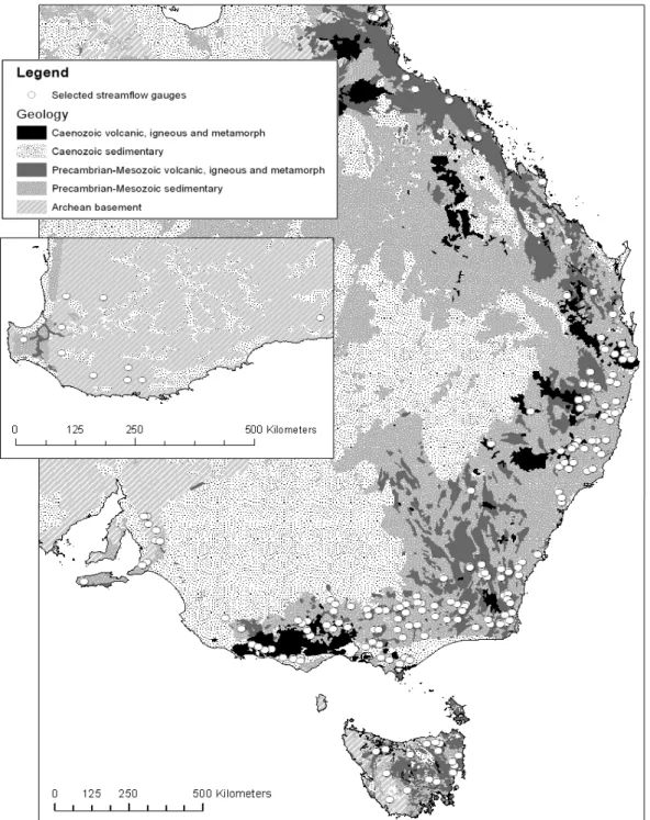
Fig. 1.The location of the 183 streamflow gauges selected in this study, and the underlying geology. Vector image provided separately.
other than rainfall was insignificant. The data set includes catchments under native forest, catchment fully cleared for grazing, and catchments with a varying combination of crop-ping, grazing, plantation forestry and native vegetation.
3.2 Parameter estimation
The parameter(s) of the linear and non-linear reservoir mod-els were found by fitting Eqs. (3) and (4), respectively, to
the available data pairs using a multi-start downhill simplex search method. The fitting criterion was the mean relative error (ε), expressed as:
ε=1
n X
Qest
Q −1
(6)
QBF= QBF,b QBF= QBF,f QBF= Q QBF= QBF,f QBF= QBF,b
Q< Q* N
Y
QBF,b> QBF,f N
Y
QBF,b< Q N
Y
QBF,f< Q N
Y
recession ascension
min(QBF,b,QBF,f)>Q N
Y
QBF= QBF,b QBF= QBF,f QBF= Q QBF= QBF,f QBF= QBF,b
Q< Q* N
Y
QBF,b> QBF,f N
Y
QBF,b< Q N
Y
QBF,f< Q N
Y
recession ascension
min(QBF,b,QBF,f)>Q N
Y
Fig. 2.Decision tree used in baseflow separation, whereQis streamflow,Q∗streamflow the previous day, andQBF,bthe backward,QBF,f
the forward andQBFthe adopted baseflow estimate, respectively.
To investigate how the size of the data masking periodTQF influenced the results, the analysis was performed using a range ofTQFvalues for six stations selected to represent the geographical and climate range in the data set.
3.3 Model selection
To decide the optimal balance between the number of fitting parameters and explained variation in observations, a version of Akaike’s Final Prediction Error Criterion (FPEC; Akaike, 1970) was calculated and interpreted. FPEC estimates the prediction error if the model was tested on a different data set and therefore the most accurate model should have the small-est FPEC. FPEC can be expressed as the product of an em-pirically estimated prediction error and a penalization factor that considers the degrees of freedomd (the number of free parameters) with the number of observationsn(the number of data pairs). Provided thatn >> d, FPEC is approximated by:
FPEC=1+d
n
1−d
nε (7)
In principle, the model with the lowest FPEC should be adopted. For example, forn=50 (the lowest number of sam-ples considered to produce a valid analysis), it follows that each additional parameter would need to explain another 4% of the residual error. Schoups et al. (2008) pointed out that this approach requires thatnis very large or else may lead to underestimates of prediction error and favour overly complex models. This caveat was considered when interpreting FPEC values. The FPEC was not the only criterion used in decid-ing on appropriate model structure. Other factors considered were: (i) the number of stations for which the alternate model structure appeared to be better; (ii) any relationships between the number of data pairs and FPEC; (iii) the degree to which parameter values could be correlated to catchment attributes
(increasing the likelihood of predictive performance in un-gauged catchments); and (iv) the correlation between fitted parameters (as an indicator of potential parameter equiva-lence).
3.4 Baseflow separation
Using the chosen reservoir model and derived parameter val-ues, the baseflow component of streamflow was estimated by combining forward and backward recursive filters. It was as-sumed that the very first and very last value in the streamflow time series represented baseflow only (associated errors were negligible).
Starting at the second last value of the stream flow time series (i=N–1) and moving backwards through the record, baseflow for time stepi was estimated by considering for-ward and backfor-ward BF estimates. The forward estimate
QBF,fis given by Eq. (3) for a linear reservoir and Eq. (4) for a non-linear reservoir; whereQ(i–1) equalled zero,QBF,f(i) was also given a value of zero. The backward estimateQBF,b for a linear reservoir is given by inversion of Eq. (3) as:
QBF,b(i)=exp(kBF)QBF(i+1) (8)
and for a non-linear reservoir as (cf. Eq. (4); Wittenberg, 1999):
QBF,b(i)=
[QBF(i+1)]b−1+
b−1
ab b−11
(a)
)
0 5 10 15 20 25
s
tr
e
a
m
f
lo
w
(
m
m
/d
)
daily streamflow
daily basef low
(b)
)
0.01 0.1 1 10 100
s
tr
e
a
m
f
lo
w
(
m
m
/d
)
daily streamflow
daily basef low
Fig. 3. Example of separation of daily streamflow into baseflow
and storm flow using a linear baseflow reservoir , plotted on(a)a linear vertical scale and(b)a logarithmic vertical scale (data chosen arbitrarily to illustrate concepts; represent 60 days in winter 1990; gauge 410705, Molonglo River @ Burbong Bridge).
3.5 Spatial predictors of streamflow response
The streamflow response descriptors analysed were the reser-voir model parameters (kBFandβ), BFI, and average QF and BF. Only categorical information was available on geology (Fig. 1). The mean and standard deviation of the values for catchments within each geological category were compared for statistically significant differences.
For other catchment characteristics continuous data was available, including measures of catchment morphology (catchment size, mean slope, flatness); soil characteristics (saturated hydraulic conductivity, dominant texture class value, plant available water content, clay content, solum thickness); climate indices (mean precipitationP, mean po-tential evapotranspiration E0, humidity index H =P /E0, remotely sensed actual evapotranspiration, average monthly excess precipitation); and land cover characteristics (fraction woody vegetation, fractions non-agricultural land, grazing land, horticulture, and broad acre cropping, remotely sensed
vegetation greenness). Data sources are listed in the supple-mentary material (http://www.hydrol-earth-syst-sci.net/14/ 159/2010/hess-14-159-2010-supplement.pdf). The analysis involved step-wise regression: potential predictors of varia-tion in the response descriptor were chosen based on para-metric and non-parapara-metric (ranked) correlation coefficients (r andr∗, respectively). A threshold of±0.40 (equivalent tor2=0.20) was considered a potentially meaningful correla-tion. Linear, logarithmic, exponential and power regression equations were calculated for all potential predictors, and the most powerful one selected. The residual variance was cal-culated and expressed both as absolute and relative residuals, after which the same procedure was repeated.
When no further variation could be explained by the catch-ment attributes, the spatial correlation in the remaining resid-ual variance was investigated using semi-variograms. A min-imum of 100 unique member data points was used for each variogram estimator point and a spherical, exponential or linear semi-variogram model was visually selected and fit-ted. The ratio of sill over the sum of sill and nugget was interpreted as the fraction of total variance that appeared spatially correlated, and the range of the variogram model was interpreted as the characteristic length scale of correla-tion. The same semi-variogram analysis was also was per-formed for the various catchment attributes (see supplemen-tary material, http://www.hydrol-earth-syst-sci.net/14/159/ 2010/hess-14-159-2010-supplement.pdf). The range of the variogram was interpreted as the characteristic length scale of correlation, suggesting that available data on soils, to-pography, major land uses and vegetation cover had typi-cal correlation lengths of 100 to 300 km, whereas climate and potential evaporation showed length scales of 300 to 700 km. The semi-variogram suggested no spatial correla-tion in catchment size or the area with different crops.
4 Results
4.1 Parameter estimation
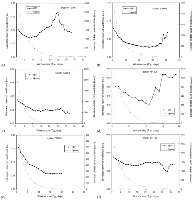
The influence of the choice of masking periodTQF on cal-culatedkBFvalues and the number of available data pairs is illustrated for six stations in Fig. 4a–f. CalculatedkBF falls rapidly asTQF is increased to 7–14 days, and a minimum value is calculated if TQF is set to 7–28 days (Fig. 4a and b, respectively). The number of available data pairs reduces exponentially as greaterTQFvalues are chosen, and no data remains forTQFof 20–40 days (Fig. 4b and d, respectively). ForTQF values greater than 10 days calculatedkBF values show variable and sometimes complex trends (e.g. Fig. 4a and f), but the remaining number of data pairs becomes in-creasingly small and likely to be associated with a single or small number of long baseflow recessions. Overall, setting
(a)
a
0.00 0.05 0.10 0.15 0.200 5 10 15 20 25 30 35 40
Window size (TBF, days)
E s ti m a te d r e s e rv o ir c o e ff ic ie n t (
kBF
) 0 500 1000 1500 2000 2500 3000 N u m b e r o f d a ta p a ir s a v a il a b le ( N p a ir s ) kBF Npairs station 410705 (b)
b
0.00 0.05 0.10 0.150 10 20 30 40 50
Window size (TBF, days)
E s ti m a te d r e s e rv o ir c o e ff ic ie n t ( k B F ) 0 500 1000 1500 2000 2500 N u m b e r o f d a ta p a ir s a v a il a b le ( Np a ir s ) kBF Npairs station 205002 (c)
c
0.00 0.05 0.10 0.15 0.200 5 10 15 20 25 30 35 40
Window size (TBF, days)
E s ti m a te d r e s e rv o ir c o e ff ic ie n t ( kB F ) 0 500 1000 1500 2000 2500 N u m b e r o f d a ta p a ir s a v a il a b le ( N p a ir s ) kBF Npairs station 120216 (d)
d
0.00 0.05 0.10 0.15 0.20 0.25 0.300 5 10 15 20
Window size (TBF, days)
E s ti m a te d r e s e rv o ir c o e ff ic ie n t ( k B F ) 0 200 400 600 800 1000 1200 N u m b e r o f d a ta p a ir s a v a il a b le ( Np a ir s ) kBF Npairs station 401008 (e)
e
0.00 0.05 0.10 0.15 0.200 5 10 15 20 25 30
Window size (TBF, days)
E s ti m a te d r e se rv o ir c o e ff ic ie n t ( k B F ) 0 100 200 300 400 500 600 700 800 900 N u m b e r o f d a ta p a ir s a v a ila b le ( N p a ir s ) kBF Npairs station 210061 (f)
f
0.00 0.05 0.10 0.150 5 10 15 20 25 30 35 40
Window size (TBF, days)
E s ti m a te d r e s e rv o ir c o e ff ic ie n t ( k B F ) 0 500 1000 1500 2000 2500 3000 N u m b e r o f d a ta p a ir s a v a il a b le ( Np a ir s ) kBF Npairs station 614196
Fig. 4.ExamplekBFvalues derived (closed lines) and number ofQ/Q∗pairs (dotted line) as the length of the storm flow masking window
TBFis increased from zero to 50 days. The six stations shown were selected to cover different geographical areas and climate regimes.
Fitting the linear reservoir model produced an average
kBF of 0.0596 (st. dev.±0.0288), implying a half-time of about 12 days. Values appeared approximately log-normally distributed (Fig. 5) and 80% of values were in the range 0.030–0.095 (i.e. half-times of 7–23 days). Fitting a non-linear reservoir produced a median β value of 0.95. The distribution was strongly skewed; 50% of values were be-tween 0.82–1.26 and 80% of values bebe-tween 0.70–1.83 (Fig. 5). Seemingly unrealistic values of β≥4 were de-rived for eight stations and values ofβ≤0.50 found for four
Table 1.Summary of the analysis of variance in values derived from baseflow separation for the 183 catchments. Listed are the fraction of variance explained by catchment attributes, the residual variance showing spatial correlation and the remaining unexplained variance. Also listed are the range (km) of the fitted semi-variograms (provided in supplementary material, http://www.hydrol-earth-syst-sci.net/14/159/ 2010/hess-14-159-2010-supplement.pdf).
Fraction of variance
Variable Symbol Attributed Spatially correlated Unexplained Range (km)
Recession coefficient kBF 27% 53% 20% 200 Baseflow index BFI 34% 53% 13% 300 Base flow QBF 84% 0% 16% n/a Quick flow QQF 70% 20% 10% 400
0.001 0.01 0.1 1 10 100
kBF (l) kBF (nl) ß (nl)
P
a
ra
m
e
te
r
v
a
lu
e
Fig. 5.Distribution of derived parameter values (N=183), from left
to right,kBFfor a linear reservoir (l) and for a non-linear reservoir (nl) and the fitted value ofβfor the non-linear reservoir. Shown are the mean (open dot), minimum and maximum (closed dots), 10– 90% range (white bars), and the 25, 50 and 75% percentiles (shaded bars). Note logarithmic vertical axis.
4.2 Model selection
The linear reservoir produced a median FPEC of 0.0306 and the non-linear reservoir a median FPEC of 0.0294, suggest-ing that the non-linear reservoir model reduced estimation er-ror by 4%. The linear reservoir produced lower FPEC scores for 131 out of 183 stations, however. The parameterβcould not be correlated to any catchment attribute (the greatestr∗
was−0.31 withE0). Values were within 20% of unity for 88 out of 183 stations, and outside the range of 0.5–4 for 12 stations. For the purposes of this study, these findings were considered insufficient basis to prefer the more complex and less robust non-linear reservoir model over the simpler lin-ear reservoir model. Results presented from here onwards were obtained using the linear reservoir model unless stated otherwise.
4.3 Streamflow components
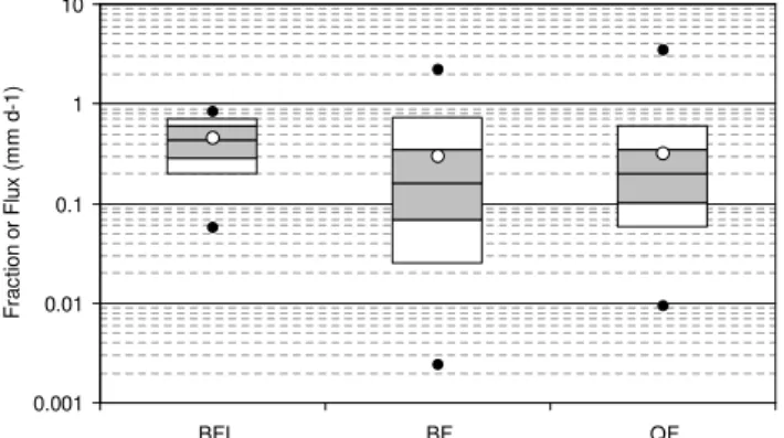
The distribution of catchment baseflow index (BFI) values appeared normal by approximation, with an average BFI of 0.45 (st. dev.±0.19; Fig. 6). The average BFI calculated
0.001 0.01 0.1 1 10
BFI BF QF
F
ra
c
tio
n
o
r
F
lu
x
(
m
m
d
-1
)
Fig. 6.Distribution of values of (from left to right) baseflow index
(BFI), average baseflow (BF) and average quick flow (QF, both in mm d−1)derived by baseflow separation using a linear reservoir. Shown are the mean (open dot), minimum and maximum (closed dots), 10–90% range (white bars), and the 25, 50 and 75% per-centiles (shaded bars). Note the logarithmic vertical axis.
using the non-linear reservoir model was 0.42±0.21. The median relative difference between the two BFI estimates was 5%, and the absolute error less than 0.10 for 162 out of 183 stations (including the 12 that had unrealistic values ofβ) The distribution of baseflow and quick flow averages was positively skewed. Median baseflow was 0.16 mm d−1 and median quick flow 0.20 mm d−1(Fig. 6).
4.4 Spatial predictors of streamflow response
The results of step-wise regression and semi-variogram anal-ysis are summarised in Table 1. Statistical analanal-ysis suggested no significant differences between different geology classes for any of the streamflow response descriptors.
y = 0.0470x-0.5076 R2 = 0.2678
0.00 0.05 0.10 0.15 0.20
0 1 2 3 4
H
k
B
F
Fig. 7. Regression between humidity index H and the linear
recession coefficientkBF.
residual variance) was spatially correlated with a charac-teristic length scale of 200 km (see supplementary material for all semi-variograms, http://www.hydrol-earth-syst-sci. net/14/159/2010/hess-14-159-2010-supplement.pdf). The remaining 20% of variance remained unexplained.
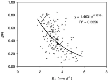
The best predictor of BFI was potential evapotranspira-tion (E0,r∗= −0.55), but humidity, precipitation-weighted monthly humidity index, and the coefficient of variance in monthly precipitation were similarly good predictors (r∗=0.51–0.54). An exponential relationship explained 34% of the variance, having a standard error of estimate of±0.16 (Fig. 8). The residual variance was not explained by the remaining attributes, but another 53% of variance (81% of residual variance) was spatially correlated with a character-istic length scale of 300 km. The remaining 13% of variance was left unexplained.
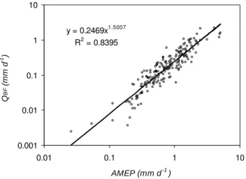
The best predictor of BF was average monthly excess pre-cipitation (AMEP,r*=0.91), followed by H (r∗=0.88) and
average rainfall and precipitation-weighted monthly humid-ity index (both r∗=0.84). A power relationship explained 84% of the variance (Fig. 9). The residual variance appeared spatially uncorrelated.
The best predictor of QF was rainfall (r∗=0.70); a power relationship explained 70% of the variance (Fig. 10). The coefficient of variation in monthly precipitation (r∗=0.36) and rainfall-weighted event precipitation (r∗=0.35) were the strongest predictors of the residual variance, but including them did not improve estimates. Another 20% of total vari-ance (66% of residual varivari-ance) was spatially correlated over length scales of 400 km. The remaining 10% of variance was left unexplained.
y = 1.4631e-0.3839x
R2 = 0.3356
0.00 0.20 0.40 0.60 0.80 1.00
0 2 4 6 8
E0 (mm d -1
)
B
F
I
Fig. 8. Regression between E0 and the period average baseflow
index BFI.
5 Discussion
5.1 Selection of storm flow window
Streamflow during the first 7 to 10 days after storm flow events appeared to include rapid drainage of stores associated with the storm event, with longer recession times occurring in wetter catchments. The gradual increase in calculatedkBF when the masking periodTQFwas increased beyond 10 to 30 days may reflect non-linear storage behaviour in the remain-ing low flow regime, but may also be caused by the greater influence of stream and riparian evapotranspiration losses in this regime (see below). The number of available data pairs often became very small as window size was increased fur-ther, introducing uncertainty and bias into the analysis. A window of 10 days was considered a reasonable compromise. The examples shown indicate that there is usually still some uncertainty.
5.2 Linear and non-linear storage behaviour
Fitting a linear reservoir produced results that were similar when compared to those obtained with a non-linear reser-voir. The derivedβ values were generally close to unity and the use of an additional parameter did little to explain more variance in the observations. In addition, resulting parame-ter estimates sometimes appeared unrealistic. Baseflow sep-aration using a linear reservoir also produced estimates of baseflow that were very similar to those obtained with a non-linear reservoir. Overall, for the purposes of this study there was considered to be little benefit from applying the more complex non-linear reservoir model.
y = 0.2469x1.5007 R2 = 0.8395
0.001 0.01 0.1 1 10
0.01 0.1 1 10
AMEP (mm d-1)
Q
B
F (
m
m
d
-1 )
Fig. 9. Regression between average monthly excess precipitation
(AMEP) and the period average baseflow (BF in mm d−1) (note double logarithmic scale).
Weisman (1977) and Tallaksen (1995), Wittenberg and Siva-palan (1999) argued that evapotranspiration from the river and riparian zone will lead to an accelerating recession at low baseflow levels, leading to fitted values of β <1. Af-ter controlling for this effect, they found values of β be-tween 2 and 3 (b=0.3–0.5). Similar values are commonly found in other countries and could be physically explained by convergence of flow paths (Chapman, 2003; Wittenberg, 1999). Where riparian evapotranspiration affects baseflow noticeably, seasonal differences in recession rates may also be expected (cf. Wittenberg and Sivapalan, 1999)
5.3 Predictability of recession coefficient
Of the variance inkBF between stations, 27% could be at-tributed to humidity, 53% was correlated over length scales indicative of terrain factors (ca. 100 km), and 20% remained unexplained (Table 1). A priori, correlation might be ex-pected with catchment size or geology, but no such relation-ship appeared to exist. On theoretical arguments, Zecharias and Brutsaert (1988) argued that the recession coefficientkBF should be proportional to:
kBF∝
KDα
Y L (10)
whereKis hydraulic conductivity,Daquifer thickness,αis slope,Y is storativity, andLa characteristic flow path length. Zecharias and Brutsaert (1988) and Brandes et al. (2005) found that geomorphological indices such as drainage den-sity (a proxy forL), slope and hydrologic soil class (perhaps a proxy forKandS)together explained about 70–80% of the variation inkBF for catchments in the Appalachians (USA).
In the current study, catchment-average saturated conductiv-ity and slope estimates were available and showed weak cor-relations withkBF(r* of−0.30 and−0.41, respectively), but
y = 0.0185x2.5079 R2 = 0.6952
0.001 0.01 0.1 1 10
1 1
P (mm d-1)
Q
QF
(
mm d
-1 )
0
Fig. 10.Regression between average precipitation (P) and the
pe-riod average quick flow (QF in mm d−1).
these relationships were opposite to those that would be ex-pected. This was because of their correlation with catchment humidity; after correcting for this soil conductivity and slope did not explain any residual variance. Most of the variation inkBF explained by the humidity index was for dry catch-ments (H <1) with times of less than 10 days (kBF>0.07; Fig. 7). These catchments generally had low average base-flow (<30 mm y−1)and intermittent streamflow. It is con-cluded that the value of humidity in predictingkBFis mainly due to the intermittent occurrence of (perched) groundwater tables with short half times in drier catchments.
The influence of perched groundwater tables, as well as perhaps the large geographical area and wide climate and ge-ology range covered by the 183 catchments, may have pre-vented detection of the influence of hydrogeology and ge-omorphology onkBF. The finding that there was consider-able correlation ofkBF over a relatively short length scales of 200 km does suggest that there are spatial terrain factors underlying the variation inkBF, but these were not captured in the catchment data available.
5.4 Predictability of base flow index
combination of catchment-average slope, topographic wet-ness index, rainfall, and soil conductivity. In the current analysis, direct evidence for a relationship between BFI and catchment-attributes relating to geomorphology or soils was not found, but there was considerable correlation over up to 150 km that may reflect undescribed terrain factors.
5.5 Predictability of average baseflow and storm flow
The overriding importance of rainfall and catchment hu-midity in determining total streamflow is well documented (e.g. Oudin et al., 2008; van Dijk et al., 2007; Zhang et al., 2004). The current analysis shows that this extends to both BF and QF components. The standard error of esti-mate (SEE) using the first order regression models shown in Figs. 8 and 10 in different combinations to estimate baseflow and quick flow were both of similar magnitude but errors ap-peared uncorrelated. Estimates of BF were slightly more ro-bust than QF estimates (SEE 70–87 vs. 89–94 mm y−1; mean relative error 37–45 vs. 52–63%; r*=0.89–0.92 vs. 0.67– 0.76).
The empirical relationships derived provide some insight into the main drivers of spatial patterns in average baseflow, storm flow, and base flow index. The stronger explanatory value of monthly rainfall excess in predicting BF suggests that seasonality in rainfall relative toE0 may be important in determining baseflow generation. Average quick flow showed a strongly non-linear relation with rainfall (exponent of 2.51; Fig. 10). This flow component could include several runoff generation mechanisms, including infiltration and sat-uration excess surface runoff and subsurface storm flow. Cor-respondingly, a multitude of factors may affect quick flow generation, including rainfall intensity distribution, factors affecting soil infiltration capacity (soil type but also land use and management), factors affecting saturated catchment area (antecedent groundwater level, geomorphology) and soil sat-uration (soil conductivity and structure, antecedent soil water content). It may be assumed that average rainfall intensity is positively related to total rainfall, whereas groundwater level and soil moisture content are likely to be higher in wet-ter catchments, providing several alwet-ternative hypotheses to explain the non-linear relationship between rainfall and QF found here.
6 Conclusions
Daily streamflow data for 183 catchments across Australia were used to estimate baseflow and quick flow contributions. Both linear and non-linear reservoirs were evaluated. Varia-tions in reservoir parameters, baseflow index (BFI) and av-erage baseflow and quick flow between the stations were analysed and where possible related to the climate, terrain and land cover attributes of the catchments using step-wise regression and semi-variogram techniques. The following conclusions are drawn:
1. A one-parameter linear reservoir produced estimates of baseflow that were as good as those obtained us-ing a two-parameter non-linear reservoir. Because it had fewer parameters and parameter values that were less variable the linear reservoir model was considered preferable for the purposes of this study.
2. The transition from storm flow dominated streamflow to baseflow dominated streamflow generally appeared to occur between 7 and 10 days after storm events. The 183 catchments showed baseflow half-times of around 12 days, with 80% of stations having half-times of 7 to 23 days. Catchment humidity explained 27% of the variation in derived recession coefficients. The shortest half-times occurred in the driest catchments and were attributed to the occurrence of fast-draining (perched) groundwater.
3. Median BFI was 0.45, with considerable variation between stations. About half (53%) of the unex-plained variance in recession coefficients and BFI val-ues showed spatial correlation over scales of 100– 150 km, probably associated with terrain factors that were not captured in the available data. The remain-ing 16–20% of variance inkBFand BFI remained unex-plained.
4. Most (84%) of the variation in average baseflow be-tween stations could be explained by monthly precip-itation in excess ofE0. Most (70%) of the variation in average quick flow between stations could be explained by average rainfall. Of the remaining variation, 20% was spatially correlated over spatial scales of∼200 km, and this may reflect a combination of terrain and climate factors. The remaining 10–16% was left unexplained. It is concluded that catchment streamflow response can be predicted quite well on the basis of catchment climate alone. The prediction of baseflow recession response should be im-proved further if relevant substrate properties were identified and measured.
Acknowledgements. This work is part of the water information
research and development alliance between CSIRO’s Water for a Healthy Country Flagship and the Bureau of Meteorology. The streamflow and catchment attribute data set used in this study was brought together by Juan Pablo Guerschman, Jorge Pe˜na Arancibia, Yi Liu and Steve Marvanek of CSIRO Land and Water; their effort is gratefully acknowledged. This manuscript has benefited considerably from comments by Zahra Paydar and Cuan Petheram (CSIRO Land and Water), three anonymous referees and the subject editor.
References
Akaike, H.: Statistical predictor identification Ann. Inst. Stat. Math., 22, 203–217 doi:10.1007/BF02506337, 1970.
Bergstr¨om, S.: Bergstrom, S.: The HBV model – its structure and applications, Report RH No. 4, Swedish Meteorological and Hydrological Institute, Hydrology, Norrkping, Sweden, 35 pp. 1992.
Beven, K.: Prophecy, reality and uncertainty in distributed hydro-logical modelling, Adv. Water Resour., 16, 41–41, 1993. Bl¨oschl, G. and Sivapalan, M.: Scale issues in hydrological
mod-elling: A review, Hydrol. Process., 9, 251–290, 1995.
Brandes, D., Hoffmann, J. G., and Mangarillo, J. T.: Base flow recession rates, low flows, and hydrologic features of small wa-tersheds in Pennsylvania, USA, J. Am. Water Resour. As., 41, 1177–1186, 2005.
Burnash, R. J. C., Ferral, R. L., and McGuire, R.: A Generalized Streamflow Simulation System-Conceptual Modeling for Digital Computers, U.S. Department of Commerce, National Weather Service and State of California, Department of Water Resources, 1973.
Chapman, T.: A comparison of algorithms for stream flow recession and baseflow separation, Hydrol. Process., 13, 701–714, 1999. Chapman, T. G.: Modelling stream recession flows, Environ.
Mod-ell. Softw., 18, 683–692, 2003.
Chiew, F. H. S., Peel, M. C., and Western, A. W.: Application and testing of the simple rainfall-runoff model SIMHYD, in: Math-ematical Models of Small Watershed Hydrology and Applica-tions, edited by: Singh, V. P. and Frevert, D. K., Water resources Publication Littleton, Colorado, USA, 335–367, 2002.
Coutagne, A.: Etude g´en´erale des variations de d´ebits en fonction des facteurs qui les conditionnent, 2´eme partie: les variations de d´ebit en p´eriode non infuenc´ee par les pr´ecipitations, La Houille Blanche, 416–436, 1948.
Guerschman, J.-P., Van Dijk, A. I. J. M., McVicar, T. R., Van Niel, T. G., Li, L., Liu, Y., and Pe˜na-Arancibia, J.: Water balance esti-mates from satellite observations over the Murray-Darling Basin, CSIRO, Canberra, Australia, 93 pp., 2008.
Haberlandt, U., Kl¨ocking, B., Krysanova, V., and Becker, A.: Re-gionalisation of the base flow index from dynamically simulated flow components – a case study in the Elbe River Basin, J. Hy-drol., 248, 35–53, 2001.
Jakeman, A. J. and Hornberger, G. M.: How much complexity is warranted in a rainfall-runoff model?, Water Resour. Res. 29, 2637–2649, 1993.
Merz, R. and Bl¨oschl, G.: Regionalisation of catchment model pa-rameters, J. Hydrol., 287, 95–123, 2004.
Nathan, R. J. and McMahon, T. A.: Evaluation of automated tech-niques for base flow and recession analyses, Water Resour. Res., 26, 1465–1473, 1990.
Oudin, L., Andr´eassian, V., Lerat, J., and Michel, C.: Has land cover a significant impact on mean annual streamflow? An in-ternational assessment using 1508 catchments, J. Hydrol., 357, 303–316, 2008.
Peel, M. C., Chiew, F. H. S., Western, A. W., and McMahon, T. A.: Extension of Unimpaired Monthly Streamflow Data and Re-gionalisation of Parameter Values to Estimate Streamflow in Un-gauged Catchments. Report prepared for the Australian National Land and Water Resources Audit., Centre for Environmental Ap-plied Hydrology, The University of Melbourne, 2000.
Santhi, C., Allen, P. M., Muttiah, R. S., Arnold, J. G., and Tuppad, P.: Regional estimation of base flow for the conterminous United States by hydrologic landscape regions, J. Hydrol., 351, 139– 153, 2008.
Schoups, G., van de Giesen, N. C., and Savenije, H. H. G.: Model complexity control for hydrologic prediction, Water Resour. Res., 44, W00B03, doi:10.1029/2008WR006836, 2008. Sivapalan, M., Takeuchi, K., Franks, S. W., Gupta, V. K.,
Karam-biri, H., Lakshmi, V., Liang, X., McDonnell, J. J., Mendiondo, E. M., O’Connell, P. E., Oki, T., Pomeroy, J. W., Schertzer, D., Uhlenbrook, S., and Zehe, E.: IAHS Decade on Predictions in Ungauged Basins (PUB), 2003–2012: Shaping an exciting fu-ture for the hydrological sciences, Hydrol. Sci. J., 48, 857–880, doi:10.1623/hysj.48.6.857.51421, 2003.
Tallaksen, L. M.: A review of baseflow recession analysis, J. Hy-drol., 165, 349–370, 1995.
van Dijk, A. I. J. M., Hairsine, P. B., Arancibia, J. P., and Dowl-ing, T. I.: Reforestation, water availability and stream salinity: A multi-scale analysis in the Murray-Darling Basin, Australia, Forest Ecol. Manag., 251, 94–109, 2007.
Wagener, T. and Wheater, H. S.: Parameter estimation and region-alization for continuous rainfall-runoff models including uncer-tainty, J. Hydrol., 320, 132–154, 2006.
Weisman, R. N.: The effect of evapotranspiration on streamflow recession, Hydrol. Sci. Bull., XXII, 371–377, 1977.
Wittenberg, H.: Baseflow recession and recharge as nonlinear stor-age processes, Hydrol. Process., 13, 715–726, 1999.
Wittenberg, H. and Sivapalan, M.: Watershed groundwater balance estimation using streamflow recession analysis and baseflow sep-aration, J. Hydrol., 219, 20–33, 1999.
Zecharias, Y. B. and Brutsaert, W.: Recession characteristics of groundwater outflow and baseflow from mountainous water-sheds, Water Resour. Res., 24, 1651–1658, 1988.