Estimating and forecasting the volatility of Brazilian finance series using arch models (Preliminary Version)

❊♥s❛✐♦s ❊❝♦♥ô♠✐❝♦s

❊s❝♦❧❛ ❞❡ Pós✲●r❛❞✉❛çã♦ ❡♠ ❊❝♦♥♦♠✐❛ ❞❛ ❋✉♥❞❛çã♦ ●❡t✉❧✐♦ ❱❛r❣❛s

◆◦ ✸✹✼ ■❙❙◆ ✵✶✵✹✲✽✾✶✵

❊st✐♠❛t✐♥❣ ❛♥❞ ❋♦r❡❝❛st✐♥❣ t❤❡ ❱♦❧❛t✐❧✐t② ♦❢

❇r❛③✐❧✐❛♥ ❋✐♥❛♥❝❡ ❙❡r✐❡s ❯s✐♥❣ ❆r❝❤ ▼♦❞❡❧s

✭Pr❡❧✐♠✐♥❛r② ❱❡rs✐♦♥✮

❏♦ã♦ ❱✐❝t♦r ■ss❧❡r

❖s ❛rt✐❣♦s ♣✉❜❧✐❝❛❞♦s sã♦ ❞❡ ✐♥t❡✐r❛ r❡s♣♦♥s❛❜✐❧✐❞❛❞❡ ❞❡ s❡✉s ❛✉t♦r❡s✳ ❆s

♦♣✐♥✐õ❡s ♥❡❧❡s ❡♠✐t✐❞❛s ♥ã♦ ❡①♣r✐♠❡♠✱ ♥❡❝❡ss❛r✐❛♠❡♥t❡✱ ♦ ♣♦♥t♦ ❞❡ ✈✐st❛ ❞❛

❋✉♥❞❛çã♦ ●❡t✉❧✐♦ ❱❛r❣❛s✳

❊❙❈❖▲❆ ❉❊ PÓ❙✲●❘❆❉❯❆➬➹❖ ❊▼ ❊❈❖◆❖▼■❆ ❉✐r❡t♦r ●❡r❛❧✿ ❘❡♥❛t♦ ❋r❛❣❡❧❧✐ ❈❛r❞♦s♦

❉✐r❡t♦r ❞❡ ❊♥s✐♥♦✿ ▲✉✐s ❍❡♥r✐q✉❡ ❇❡rt♦❧✐♥♦ ❇r❛✐❞♦ ❉✐r❡t♦r ❞❡ P❡sq✉✐s❛✿ ❏♦ã♦ ❱✐❝t♦r ■ss❧❡r

❉✐r❡t♦r ❞❡ P✉❜❧✐❝❛çõ❡s ❈✐❡♥tí✜❝❛s✿ ❘✐❝❛r❞♦ ❞❡ ❖❧✐✈❡✐r❛ ❈❛✈❛❧❝❛♥t✐

❱✐❝t♦r ■ss❧❡r✱ ❏♦ã♦

❊st✐♠❛t✐♥❣ ❛♥❞ ❋♦r❡❝❛st✐♥❣ t❤❡ ❱♦❧❛t✐❧✐t② ♦❢ ❇r❛③✐❧✐❛♥ ❋✐♥❛♥❝❡ ❙❡r✐❡s ❯s✐♥❣ ❆r❝❤ ▼♦❞❡❧s ✭Pr❡❧✐♠✐♥❛r② ❱❡rs✐♦♥✮✴

❏♦ã♦ ❱✐❝t♦r ■ss❧❡r ✕ ❘✐♦ ❞❡ ❏❛♥❡✐r♦ ✿ ❋●❱✱❊P●❊✱ ✷✵✶✵ ✭❊♥s❛✐♦s ❊❝♦♥ô♠✐❝♦s❀ ✸✹✼✮

■♥❝❧✉✐ ❜✐❜❧✐♦❣r❛❢✐❛✳

Estimating and Forecasting the Volatility of

Brazilian Finance Series Using ARCH Models

¤

João Victor Issler

Graduate School of Economics - EPGE

Getulio Vargas Foundation

Praia de Botafogo 190 s. 1125

Rio de Janeiro, RJ 22253-900

Brazil

Preliminary version, please do not quote. March, 1999

A bst r act

The goal of this paper is to present a comprehensive emprical anal-ysis of the return and conditional variance of four Brazilian …nancial series using models of the ARCH class. Selected models are then compared regarding forecasting accuracy and goodness-of-…t statis-tics. To help understanding the empirical results, a self-contained theoretical discussion of ARCH models is also presented in such a way that it is useful for the applied researcher. Empirical results show that although all series share ARCH and are leptokurtic relative to the Normal, the return on the US$ has clearly regime switching and no asymmetry for the variance, the return on COCOA has no asymmetry,

¤_{This paper wasprepared for t heInvited Session on volatility of theSociedadeBrasileira}

while the returns on the CBOND and TELEBRAS have clear signs of asymmetry favoring the leverage e¤ect. Regarding forecasting, the best model overall was the EGARCH (1; 1) in its Gaussian version. Regarding goodness-of-…t statistics, the SW ARCH model did well, followed closely by the Student-t GARCH (1; 1).

1 I nt r oduct ion

ARCH - Autoregressive Conditional Heteroskedasticity - is recognized today as a major feature of …nancial data which several econometric models try to capture. This paper presentsa comprehensiveempirical analysisof thereturn and conditional variance of a variety of Brazilian …nancial series using models of the ARCH class. The data used covers a wide spectrum of Brazilian Finance series: a spot stock-price index - IBOVESPA, of the São Paulo Stock Exchange, the spot price of a popular Brazilian stock - TELEBRAS, traded in the São Paulo Stock Exchange, a spot currencyexchange rate -R$/ US$, and a spot popular commodity price - COCOA. Selected models of the ARCH class for the return of these series are …tted and estimates compared regarding forecasting accuracy and goodness-of-…t statistics. To help to understand the empirical results obtained, a self-contained theoretical discussion of ARCH modelsisalso presented, focusing on econometric results of ARCH models that are useful for the applied researcher.

2 Some T heor y of A RCH M odels

In this Section selected results for ARCH models are presented. Since the literature on ARCH is vast and comprehensive, including more than one hundred papers and the surveys of Bollerslev, Chou and Kroner(1992), of Bollerslev, Engle and Nelson(1994), and the book of collected papers edited by Engle(1995), it makes little sense to repeat here theoretical results that are already discussed elsewhere at greater depth and length.

Instead, the focus of this Section is on econometric results of ARCH models that are useful for the applied researcher. In a direct analogy with the time-series method proposed by Box and Jenkins(1976), the “ identi…ca-tion” of ARCH processes is motivated here by considering autocorrelation and partial autocorrelation functions for the squared (returns of …nancial) series. We later discuss three improvements for the class of ARCH models: the generalized ARCH - GARCH , the Exponential GARCH - EGARCH , and the switching-regime ARCH model - SW ARCH , motivating their intro-duction by previous shortcomings in applying early ARCH models to actual (Finance) data. All models discussed here are later applied to Brazilian …nancial data.

2.1 A RCH : T he B asic I dea and Select ed M odels

of models that use a non-linear function. Perhaps, the most important one in Finance is the class of ARCH models introduced by Engle(1982).

Although the ARCH model and its extensions are widely applied in Fi-nance today, that was not at all its original motivation. Engle(1995, pp. xi-xii) writes that he thought that the main contribution of ARCH models would be on the Rational Expectations debate in Macroeconometrics. By the end of the 1970’s, in‡ation was soaring everywhere due to two oil shocks. This raised concerns of how well it could be forecast. Indeed, Okun(1971) and Friedman(1977) proposed that an increase in the level of in‡ation would raise its variance. Interestingly enough, using the framework of his 1982 Econometrica paper, Engle(1983) showed that the high level of U.S. in‡a-tion experienced around that time was highly predictable, and that in‡ain‡a-tion level and variance were uncorrelated.

As is the case with several successful theoretical developments in econo-metrics, Clive Granger reports that the birth of ARCH models was a conse-quenceof an observed empirical regularity. When applying thetools proposed by Box and Jenkins, one could …nd series which were unpredictable, although their squares were highly predictable. This suggested that some sort of non-linearity was at work. This lead Engle(1982) to propose the class of ARCH models, which conforms to this early empirical observation. Granger, on the other hand, went on to work with the bilinear model, which has a structure similar to that of ARCH models; see Granger and Andersen(1978).

The linear ARCH (p) model introduced by Engle can be summarized in: yt = xt¯ + "t;

"tj - t ¡ 1 » D ¡

0; ¾2 t

¢ ; ¾2

t ´ E £

"2 t j - t ¡ 1

¤

= ®0+ p X

i = 1

®i "2t ¡ i; (1)

whereD (¢) issomeparametric distribution, usually theNormal or theStudent-t, and xt is either weakly exogenous or an element of the conditioning set - t ¡ 1. Notice the similarity between the last line in (1) and an AR (p) model:

Wt = c + p X

i = 1

Á_i Wt ¡ i + ¹_t: (2)

It is easy to write an ARCH process (1) as an autoregressive process (2), using the result that "2

Martingale-Di¤erence Sequence. We have: "2

t = ®0+ ®1 "2t¡ 1+ ¢¢¢+ ®½"2t ¡ p+ ´t: (3) To ensure that "2

t ¸ 0, 8t, for all possible realizations of f "tg1_{t= 1}, it is usually assumed that (i) ®0 > 0 and ®i ¸ 0, 8i = 1; ¢¢¢; p, and that (ii) ´t has a lower bound of ¡ ®0.

The simplest linear ARCH model possible - the Gaussian ARCH (1), with ¯ = 0, allows discussing several interesting features of models in this class. It is summarized in:

Ytj - t ¡ 1 » N ¡

0; ¾2 t

¢ ¾2

t = ®0+ ®1 Yt¡ 12 : (4) Notice that if ®1 = 0, Yt j - t ¡ 1 » N (0; ®0), i.e., Yt is conditionally homo-cedastic. The theorem below shows some of its basic properties.

T heorem 1 (Engle(1982)) For integer r , the 2r th (unconditional) mo-ment of a …rst-order linear ARCH process with ®0 > 0, ®1 ¸ 0 exists if, and only if, ®r

1 r ¦

j = 1(2j ¡ 1) < 1:

Thus, the second and fourth unconditional moments are de…ned, with E (Y2

t ) = 1¡ ®®01, and E (Y

4

t ) = 3®

2 0

(1¡ ®1)2 ¢

1¡ ®2 1

1¡ 3®2

1, i¤ ®1 < 1 and 3®

2

1 < 1 re-spectively. This has two implications. First, although the conditional model is Gaussian, the unconditional distribution has fatter tails compared to the Normal1_{. This happens because} 1¡ ®21

1¡ 3®2

1 > 1. Under a Gaussian unconditional

distribution, the Kurtosis coe¢ cient is given by 3 ®20

(1¡ ®1)2, hence smaller than

3®2 0

(1¡ ®1)2 ¢

1¡ ®2 1

1¡ 3®2

1. Second, although the conditional distribution is

heteroskedas-tic, the conditional distribution is homocedastic. Indeed, because the mean and autocovariances of Yt are not time varying, this process is weakly station-ary despite displaying conditional heteroskedasticity. This result generalizes for a wider class of ARCH (p) models as below.

1_{Despite the fact that this feature of conditional normality is helpful in modelling}

T heorem 2 (Engle(1982)) The pth-order linear ARCH process with ®0> 0, ®1; ¢¢¢; ®p ¸ 0 is covariance- (weakly-) stationary if, and only if, the associated characteristic equation has all roots outside the unit circle. The stationary variance is given by ®0

1¡ §pi = 1 ®i:

This last result illustrates why the appropriate ARCH (p) model con-forms to the stylized fact that the level series (error) is white noise despite the fact that the autocorrelation and partial autocorrelation of its squares show signs of predictability. Following Bollerslev(1986), write the error term in (3) as "t = ¾t ¢zt, where zt » i:i:d: (0; 1). Based on the law of iterated expectations is easy to show that E ["t] = 0, E ["t"t ¡ j] = 0 8j > 0, and given Theorem 2, E ["2

t] = 1¡ §®pi = 10 ®i. Hence, "t is white noise. However, if we take

"2

t = ¾2t ¢zt2, it is obvious that its autocorrelations will not die out because of (3), and that its partial autocorrelation will only be zero starting at order p + 1.

Estimating an ARCH (p) process by maximum likelihood is straightfor-ward once a parametric distribution is assumed for zt in "t = ¾t ¢zt. The usual assumption is that zt has an i :i :d: Gaussian or Student-t distribution. In any case, the joint density of the sample y1; ¢¢¢; yT can be recursively factored into the conditional and marginal densities to form:

f (y1; ¢¢¢; yT; µ) = T Y

t = 1

f (ytjyt¡ 1; ¢¢¢; y¡ p+ 1; µ) ; (5)

where µ is a vector of parameters of the joint density, and we condition on pre-sample observations. For the simple ARCH (1) model discussed above we have:

f (ytjyt¡ 1; ¢¢¢; y0; µ) = p 1

2¼¢¡®0+ ®1 yt ¡ 12 ¢1=2 £

exp Ã

¡ 1 2

y2 t ¡

®0+ ®1 yt ¡ 12 ¢

!

; (6)

where µ = (®0; ®1)0. Using this result, maximum likelihood estimates can be found by numerically optimizing the conditional log-likelihood function:

logL (µ; ¢) = T ¢log µ

1 p

2¼ ¶

¡ 1 2

T X

t = 1 µ

log¡®0+ ®1 yt ¡ 12 ¢

+ yt2 ®0+ ®1y2t ¡ 1

subject to the constraints ®0> 0 and ®1 ¸ 0.

For Financial series, if one believes that outliers are clustered (e.g., Man-delbrot(1963)), then the estimation method described above reduces the im-pact of these extreme observations on parameter estimates. This happens because the denominator of y2t

®0+ ®1y2_{t ¡ 1} will reduce the contribution of a given

outlier y2

t in (7), sincey2t ¡ 1ismorelikely to belargeaswell. This shows a clear advantage for recognizing the presence of ARCH when compared to (say) the case where homocedasticity is erroneously assumed. In the latter, all observations are equally weighted in the likelihood function, whereas in the former outliers get a smaller weight. Coupled with the fact that the uncondi-tional distribution is leptokurtic relative to the Normal, allowed Engle(1982) to conclude that ARCH models show potential to deal with clustered out-liers. Of course, if outliers are not clustered, the weighting procedure will not work. Hence, Engle mentions nothing regarding outliers in general. He also makes no attempt to compare ARCH models with “ robust” estimates2_. From empirical experimentation with models in the ARCH (p) class, it became apparent that the order of the …tted model was quite large - p large. In a direct analogy with models in the AR (p) class, where the par-simonious solution is to include M A (¢) terms - forming an ARM A model, the ARCH (p) process was generalized to include these “ M A (q) terms.” This is the motivation behind the GARCH (p; q) model, proposed by Boller-slev(1986)3_:

"tj - t ¡ 1 » D ¡

0; ¾2 t

¢ ; ¾2

t = E £

"2 t j - t ¡ 1

¤ = ! +

q X

i = 1

®i"2t ¡ i + p X

i = 1 ¯_i¾2

t ¡ i

= ®0+ A (L) "t + B (L) ¾2t; (8) where A (L) = P q_{i = 1}®iLi _{and B (L) =} P p

i = 1¯iLi are …nite order polynomials on the lag operator L. To see how the solution proposed by Bollerslev mimics the ARM A class, consider for simplicity the GARCH (1; 1) model:

¾2

t = ! + ® "2t ¡ 1+ ¯ ¾2t ¡ 1: (9) If we de…ne as in (3), ´_t ´ "2

t ¡ ¾2t as the conditional variance prediction error, with the property that E [´_t j - t¡ 1] = 0, we can solve (9) in terms of

current and lagged "2

t and ´t to get: "2

t = ! + (® + ¯ ) "2t ¡ 1¡ ¯ ´t ¡ 1+ ´t; (10) which is an ARM A(1; 1) process for "2

t. Using the same principle, it is easy to show that a GARCH (p; q) model is indeed an ARM A (max (p; q) ; p) for "2

t; see Bollerslev(1986).

The Theorem below shows that the result in Theorem 2 generalizes for this wider class of ARCH models.

T heorem 3 (B oller slev(1986)) The Gaussian GARCH (p; q) process, with ! > 0, ®i, ¯i ¸ 0, 8i = 1; ¢¢¢; max [p; q], is weakly stationary with E ("t) = 0; Var ("t) = _{(1¡ A (1)¡ B (1))}! and Cov ("t; "s) = 0; t 6= s; if, and only if, A (1) + B (1) < 1:

The analogy between the ARM A and the GARCH class is also present when forecasting is considered, because the GARCH (p; q) is linear on lagged "2

t and ¾2t. For the GARCH (1; 1) model, de…ning Et¾2t+ s ´ E £

¾2 t+ sj- t

¤ as the forecast of the conditional variance for horizon s, using information up to t, we have:

Et¾2

t+ 2 = ! + (®+ ¯ ) ¾2t+ 1; and; Et + 1¾2

t+ 3 = ! + (®+ ¯ ) ¾2t + 2: (11) Taking the conditional expectation of the last line of (11) using the con-ditioning set - t, it is easy to show using the law of iterated expectations that:

Et¾2t + 3 = ! [1 + (®+ ¯ )] + (®+ ¯ )2 ¾2t+ 1 ...

Et¾2t + s = ! "

1 ¡ (®+ ¯ )s¡ 1 1 ¡ (®+ ¯ )

#

+ (® + ¯ )s¡ 1¾2

t + 1: (12) As long as the parameter-restriction and stationarity conditions in The-orem 3 hold, i.e., 0 < ® + ¯ < 1, the expression in (12) converges to the unconditional variance of "t as the forecasting horizon increases:

Et¾2 t+ s !

! 1 ¡ (® + ¯ )

¸

The Exponential GARCH - EGARCH model was proposed by Nel-son(1991) to deal with three basic shortcomings of models in the GARCH class4_{. First, the impact of shocks on volatility is symmetric for these} mod-els. Hence, positive or negative shocks have exactly the same e¤ect on the conditional variance. Since most applications of models in the GARCH class are in Finance, and for these data it is observed that the e¤ects of positive and negative returns on volatility is not identical (e.g., Black(1976)), it is desirable to conceive models that allow estimation and testing for asymme-try. Second, the restrictions ®0 > 0, ®i, ¯ i ¸ 0, 8i , constrain the roots of the characteristic polynomials of GARCH models, preventing random oscillatory behavior in ¾2

t. Moreover, when these restrictions are binding, maximum likelihood estimates are a constrained optima. Third, measures of persistence of shocks to the conditional variance for integrated GARCH processes depend on the norm considered, and no direct analogy can be made with results of the unit-root literature5_.

We consider here a simpler version of the EGARCH model proposed by Nelson:

"t = ¾t ¢zt; with; zt » i:i :d:(0; 1);

g (zt) = µzt + ° [jztj ¡ E (jztj)] ; ln¡¾2

t ¢

= ! + _¡(1 + Ã1L + ¢¢¢+ Ã1Lq)

1 ¡ Á₁L ¡ ¢¢¢¡ Á_pLp¢ ¢g (zt ¡ 1) = ! +

1 X

i = 1

¯ _ig(zt¡ i) : (14)

The third line in (14) allows for asymmetric e¤ects of shocks on the (log of the) conditional variance. When zt > 0, the slope of g (zt) is µ + ° , but for zt < 0, the slope of g(zt) is µ ¡ ° . The fourth line depicts a simple ARM A process for ln (¾2

t), proposed by Nelson as a parsimonious represen-tation for the in…nite M A process for ln (¾2

t). In his original formulation, he also considered a time varying intercept for ln (¾2

t).

T heorem 4 (light version of N elson(1991)) If at least one of the pa-rameters ° or µ are non-zero, f exp (¡ ! ) ¾2

tg, f exp (¡ ! =2) "tg, and

4_{See t he discussion in the Introduction of Nelson(1991).}

5_{For t his last point, see t he discussion in Bollerslev, Engle and Nelson(1994, pp.}

f ln (¾2

t) ¡ ! g are strictly (strongly) stationary and ergodic, and f ln (¾2t) ¡ ! g is covariance-stationary if, and only if , P 1_{i = 1}¯2

i < 1 .

It is worth noting that the ARM A speci…cation presented above is widely used in applications, being the most relevant for the applied researcher. In this case, a necessary and su¢ cient condition for P 1_{i = 1}¯2

i < 1 is that all the roots of ¡1 ¡ Á₁z ¡ ¢¢¢¡ Á_pzp¢_{= 0 lie outside the unit circle.}

For the EGARCH (1; 1) model, the (log) variance equation is:

ln¡¾2 t

¢

= ! 0_{+ ¯ ln}¡_¾2 t ¡ 1

¢ + ®

¯ ¯ ¯ ¯_¾"t ¡ 1_{t ¡ 1}

¯ ¯ ¯

¯ + °_¾"t ¡ 1_{t ¡ 1}; (15) where the model has been reparameterized with ! 0_{= (1 ¡ Á}

1) ! ¡ ° E jzt¡ 1j, and ¯ = Á₁. A slightly di¤erent speci…cation is considered in Hamilton(1994, pp. 668-669):

¡ ln¡¾2

t ¢

¡ ! ¢= ¯ ¡ln¡¾2 t¡ 1 ¢ ¡ ! ¢+ ® ¯ ¯ ¯ ¯_¾"t ¡ 1

t ¡ 1 ¯ ¯ ¯ ¯ ¡ E

¯ ¯ ¯ ¯_¾"t ¡ 1

t ¡ 1 ¯ ¯ ¯

¯ + °_¾"t ¡ 1 t ¡ 1 ¸

: (16)

In either (15) or (16) there is no asymmetry in the variance as long as ° = 0. This constitutes a testing procedure for the asymmetric e¤ect. If ° 6= 0, then there is a di¤erentiated impact of news on volatility. If ° < 0 there is the so called “ leverage e¤ect,” where good news have a smaller impact on the conditional variance than bad news; see Pagan and Schwert(1990) and Engle and Ng(1991).

Another model that allows estimating and testing the leverage e¤ect is the Threshold ARCH - TARCH model, proposed independently by Za-koian(1990), and Glosten, Jaganathan, and Runkle(1993). The speci…cation for the conditional variance is:

¾2

t = ! + ¯ ¾2t ¡ 1+ ®"2t ¡ 1+ ° ¢dt ¡ 1¢"2t ¡ 1; (17) where the dummy variable dt¡ 1 = 1, if "t ¡ 1 0, and dt ¡ 1 = 0 otherwise. Again, there is no asymmetry in the variance as long as ° = 0. Here, there is the leverage e¤ect if ° > 0.

and Lamoureux and Lastrapes(1990), one of the consequences of ignoring possible changes in regime is an overestimation of the persistence of shocks to the conditional variance. Hamilton and Susmel note that this relates “ to Perron’s(1989) observation that changes in regime may give the spurious impression of unit roots.”

Nowhere there are more changes in rules and is volatility more vari-able than in market economies. Because this feature of emerging-market …nancial data leads to potentially interesting applications of tech-niques that recognize changesin regime, wediscuss now theswitching ARCH - SWARCH model of Hamilton and Susmel. The SWARCH ¡ L (k; q) model, where the L stands for leverage (or asymmetric e¤ect), k denotes the number of regimes, and q denotes the order of the ARCH process, is given by:

ut = pgst £ eut;

eut = ¾t ¢zt; with;

zt » i :i :d:(0; 1);

¾2

t = ®0+ ®1ue2t¡ 1+ ¢¢¢+ ®qeu2t¡ q+ » ¢dt¡ 1¢eu2t¡ 1; (18)

where dt¡ 1 = 1, if eut¡ 1 0, and dt¡ 1 = 0, if eut¡ 1 > 0 is the dummy

variable for the leverage e¤ect, and st represents all the possible regimes for

the variance process. For regime one, i.e., when st = 1, the variance factor is

normalized to unity, i.e., g1= 1. When st = 2, all things equal, the variance

of ut is g2 times higher than that in regime one, and so on, up to gk, where

st = k.

As in the rest of the literature on ARCH , it is usually assumed that zt is

either Gaussian of has a Student-t distribution. It is further assumed that st

can be described by a Markov chain. The probability that there is a change in regime on t, going from regime i in t ¡ 1, to regime j , is:

Pr [st = j j st¡ 1 = i ] = pi j; (19)

where it is useful to collect all these parameters in a transition probability matrix, P = (pi j), of order k £ k. Notice that

P _k

j = 1pi j = 1. Hence, the

columns of P add up to unity. Along with the variance factors g1, g2, ¢¢¢,

gk, these probabilities are additional parameters to be estimated. In forming

2.2 Est im at ion, I nfer ence and Test ing

It is common practice to estimate the models discussed above by maximum likelihood after a parametric distribution for the error term is assumed. For applied research, since there is usually doubt about which parametric distri-bution to use, it is helpful to regard these estimates as quasi-maximum likeli-hood; see Bollerslev and Wooldridge(1992) inter-alia. There is also the pos-sibility of estimating ARCH processes by non-parametric, semi-parametric and semi-non-parametric methods; see Engle and Gonzalez-Rivera(1991) for semi-parametric methods, Hamilton(1994) for a discussion on non-parametric estimates of ARCH processes using the generalized method of moments (GMM), and Gallant and Tauchen(1989) and Gallant et al.(1991, 1992, 1993) for semi-non-parametric methods.

To perform conditional maximum likelihood estimation, …rst decompose the joint density of the sample w1; ¢¢¢; wT recursively as a product of

condi-tional densities to form:

f (w1; ¢¢¢; wT; µ) = T

Y

t= 1

f (wt jwt¡ 1; ¢¢¢; w¡ k ; µ) ; (20)

where µ is a vector of parameters of the joint density, wt is a vector that

includes the explained and explanatory variables, and conditioning on pre-sample observations up to ¡ k is implicit.

There are several examples of parametric densities that are used in prac-tice in forming (20). Bollerslev(1986) assumes conditional normality for the error term "t of the GARCH (p; q) model in (8), i.e.:

f (wt jwt¡ 1; ¢¢¢; w¡ k ; µ) = p 1

2¼¢¾t

£ exp µ

¡ 1 2

"2 t

¾2 t

¶

; (21)

whereas Bollerslev(1987) assumes that "t has a Sudent-t distribution with º

degrees of freedom and scale parameter Mt (to yield a unit variance). Hence,

f (wtjwt¡ 1; ¢¢¢; w¡ k ; µ) = ¡ [(º + 1) =2]

(¼º )1=2 ¡ [º =2]M

¡ 1=2 t 1 +

"t

Mtº

¸¡ (º + 1)=2

; (22)

where ¡ [¢] is the gamma function.

as a limiting case of the Student-t density when º ! 1 , using (22) in place of (21) allows the estimation procedure to select the number of degrees of freedom that best …ts the data, thus not ruling out leptokurtosis a priori. If the estimate of º is relatively large, then the Normal may not be a bad approximation.

Because the Sudent-t distribution, with º …nite, may imply no …nite un-conditional moments for the error process, Nelson(1991) proposes the use of the Generalized Error Distribution (GED). Its density function, for a random variable normalized to have zero mean and unit variance, is:

f (z) = º exp £

¡ 1 2jz=¸ j

º¤

¸ 2(1+ 1=º ) _{¡ [1=º ]}; (23)

where ¸ = £2(¡ 2=º ) _{¡ [1=º ] ¡ [3=º ]}¤1=2_{. As in the Student-t density, º controls}

the tickness of the distribution tail. For º = 2, the density (23) collapses to the Standard Normal, a result that can be used for a Normality test. For º < 2, it has ticker tails than the Normal and vice-versa for º > 2. For º = 1 , z is uniformly distributed on the interval £¡ 31=2_{; 3}1=2¤_.

With correct speci…cation for the functional form of

f (wt jwt¡ 1; ¢¢¢; w¡ k ; µ), the log-likelihood function can be written as:

log L (µ; ¢) =

T

X

t= 1

log(f (wt jwt¡ 1; ¢¢¢; w¡ k ; µ))

=

T

X

t= 1

lt(¢) ; (24)

where lt(¢) is the individual likelihood contribution. The function (24) is

usu-ally maximized by numerical methods subject to non-negativity constraints whenever necessary. If µ0 is the true value of the parameters in (24), where

µ02 int £ , and £ is a compact subspace of a Euclidean space such that the

error process has …nite second moments, then, under fairly general conditions (e.g., Weiss(1986)), the maximum likelihood estimate of µ, bµT, converges in

distribution as follows: p

T³bµT ¡ µ0

´

d

¡ ! N ¡0; I¡ 1 µ

¢

; (25)

where I¡ 1 µ =

h

¡ E³ @2lt(¢)

@µ @µ0

¯ ¯ ¯ - t¡ 1

´ i_{¡ 1}

estimated by³T¡ 1P T

t= 1@l@µt(¢)@l@µt(¢)0

´_{¡ 1}

, evaluated at bµT, allowing inference on

µ to be conducted using (25).

If there is doubt about the parametric density f (wtjwt¡ 1; ¢¢¢; w¡ k ; µ),

but the researcher uses the Normal density, bµT can still be regarded as

the quasi-maximum likelihood estimate of µ. In this case, inference can be conducted using the appropriate correction proposed by Bollerslev and Wooldridge(1992), which relies on:

p

T³bµT ¡ µ0

´

d

¡ ! N ¡0; D¡ 1_SD¡ 1¢_{; (26)}

where S = plim ³T¡ 1P T t= 1@l@µt(¢)

@lt(¢)

@µ0

´ , and D = plim³T¡ 1P T

t= 1¡ E

³

@2_l t(¢)

@µ @µ0

¯ ¯ ¯ - t¡ 1

´ ´

, for which consistent estimates can also be constructed making inference feasible.

Testing for ARCH can be easily performed via a Lagrange Multiplier type test proposed by Engle(1982) using the following steps6_:

1. Run an ordinary least-squares regression to get the residualsb"t. Square

them to get b"2_t.

2. Regress b"2

t on a constant and m of its own lags, obtaining R2u - the

uncentered R-squared statistic of this last regression.

3. Under the null that "t » i:i :d:N (0; ¾2), T ¢R2u d

¡ ! Â2

m. Thus, by

comparing T ¢R2

u with the appropriate entry of a Â2distribution table,

one can test the null of no ARCH .

3 Volat ilit y in Finance

Volatility is the generic name for conditional standard deviation. In Fi-nance, the term is usually employed to denote the conditional standard devi-ation of asset returns. Although this subject has evolved considerably in the last twenty years, the market-volatility measures that have been employed in practice are quite naive in statistical sense, since the heteroskedasticity 6_{Other test ing procedures are discussed in Bollerslev(1986) and in the survey of}

present in market returns is not usually recognized. Denoting by rt the

de-meaned return of a given asset, it is not uncommon for traders to use the following statistic to measure asset-return volatility:

Vt =

à N¡ 1

N ¡ 1_X

i = 0

r2 t¡ i

! 1=2

; (27)

t = N ; N + 1; ¢¢¢

Notice that (i) V2

t is the maximum likelihood estimate of the variance

of the return only if rt is homocedastic and normally distributed, and (ii)

Vt is calculated using a …xed window of N observations. Using a window

with width N generates an unpleasant property for Vt: there is a (an almost)

discrete jump for it when an extreme rt observation is either included or

excluded from the average in (27).

A second commonly used device is the exponential smoothing St for the

squared asset return:

St = (1 ¡ ¸ ) 1

X

j = 0

¸j _r2 t¡ j

= ¸ St¡ 1+ (1 ¡ ¸ ) r2t; (28)

where ¸ is the decay parameter used to smooth-out lagged squared returns, and it is assumed that 0 < ¸ < 1. This procedure is identical to the use of a convex combination of lagged St and current rt2, as shown in the last line of

(28). UsingpSt as a volatility measure makes the impact of outliers on

p St

to decrease as time passes, thus it looks smoother than Vt.

A third commonly employed volatility measure is the “ implicit volatility” derived from solving the Black and Scholes(1973) formula. A usual problem for this measure is the implicit assumption of log-Normality for the asset price, despite overwhelming empirical evidence to the contrary.

All volatility measures described above disregard the heteroskedasticity present in asset returns7_{and theautocorrelation structureof squared returns.}

Put in simple terms, they may throw out important information about cur-rent an future volatility. Here we go back full circle to Engle’s(1982) original idea on Rational Expectations: if there is information on the conditional variance of returns, why not use it?

Modelsof theARCH class recognizefrom theoutset that heteroskedastic-ity is an empirical regularheteroskedastic-ity of …nancial data. They incorporate this feature of thedata by using a simple and ingenioustime-seriesmodel8_{. In an}

interest-ing study, Noh, Engle and Kane(1994) suggest the use of ¾t =

p E ["2

t j - t¡ 1]

(where "t is the innovation in the return series) as a measure of volatility

for the return of the S&P500 index. Indeed, these authors …nd that pro…ts using GARCH (1; 1)-volatility forecasts signi…cantly exceed transaction costs for near-the-money straddles. This shows that although ARCH has a sec-ond order e¤ect on forecasting returns, money could be made by using such information.

GARCH -volatility forecasts have several interesting features. For a sta-tionary GARCH (1; 1) model, (13) and (12) above show respectively that variance forecasts (i) have mean reversion to the unconditional variance, and (ii) use the most recent information with the appropriate weights to forecast the variance into the future. Regarding the latter there is a similarity be-tween GARCH -volatility forecasts and the use of the exponential smoothing device. Starting with (9), and assuming that ®; ¯ > 0 and 0 < ® + ¯ < 1, we can solve for ¾2

t in terms of the lagged squared errors to get:

¾2 t =

!

1 ¡ ¯ + ®

1

X

i = 1

¯i ¡ 1 _"2

t¡ i; (29)

which shows that the GARCH model is a way of exponentially smoothing past return innovations; see (28) above. Indeed, if (demeaned) returns are unforecastable, (29) will be a weighted average of lagged squared returns with exponentially decreasing weights.

4 Est imat ing and For ecast ing Volat ilit y in

B r azilian Finance Ser ies

4.1 T he D at a

The data used covers a wide spectrum of Brazilian Finance series: a spot stock-price index - IBOVESPA, of the São Paulo Stock Exchange, the spot 8_{On other grounds, ARCH models were criticized because they were not derived from}

price of a popular Brazilian stock - TELEBRAS, traded in the São Paulo Stock Exchange, a spot currency-exchangerate- R$/ US$, and a spot popular commodity price - COCOA, with data extracted from the ICCO database. All asset-prices are US$ denominated and data frequency is daily (except for weekends). For the COCOA series the sample covers the period from Jan. 5th, 1990 through Jul. 1st, 1998. For the R$/ US$ and TELEBRAS series the sample covers the period from Jul. 4th, 1994 through Jul. 1st, 1998. For the CBOND series the sample period goes from Jul. 18th, 1994 through Jul. 1st, 1998.

There are some missing values for all series. Most are due to holidays. To keep the data frequency uniform across the sample (excluding weekends), missing observations were completed using the most recent quote for each series. Using the transformed data set, the percentage instantaneous return for each series was calculated using a log-di¤erence transformation, i.e., for each price series zt, 100 £ ¢ ln (zt) was computed. Plots of the data are

presented in Figure 1. As is typical of …nancial series, they all show sign of heteroskedasticity and volatility clustering.

The return of the US$ shows two distinct patterns of variation during the sample period, re‡ecting the change in regime from the wide target zones of the beginning of the Real plan to the narrow target zones implemented after the ‡oating of the Mexican Peso. With the exception of the COCOA series, which is traded abroad, all series traded in Brazil vary wildly in relativeterms during the Mexican and the Asian crises.

4.2 Est im at ion R esult s

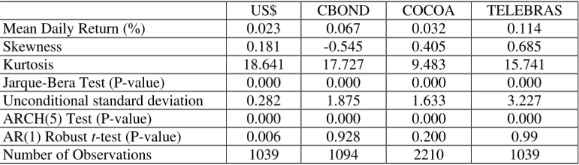
Autocorrelation and partial autocorrelation functionsfor all returns and their squares, as well as other basic statistics for the data, are presented in Ta-ble 1. Autocorrelation coe¢ cients are rather small, re‡ecting no obvious predictability. Indeed, if returns were predictable, there would be arbitrage opportunities for the average investor. Since anyone can be an average in-vestor, there can be no autocorrelation for the return9_{. The highest estimate}

for the autocorrelation coe¢ cient is 0.12. It happens for the return on the US$ at lag …ve. Compared to the benchmark of 2=pT = 2=p 1039 ' 0:06,

9_{Campbell, Lo and McKinley(1994, pp. 85-90) considered spurious autocorrelation}

it is signi…cant. However, the use of this benchmark is only valid under ho-mocedasticity. Indeed, the benchmark underestimates the approximate 95% con…denceinterval if thedata is heteroskedastic, which is probably thecase10_.

The autocorrelation coe¢ cients for squared returns show a completely di¤erent pattern, re‡ecting the fact that the conditional variance of returns is predictable. This is corroborated by the fact that all ARCH tests performed reject homocedasticity of returns with great con…dence. Also, the Jarque and Bera(1987) normality test rejects Normal returns for all series. The latter has little to do with returns having a skewed distribution, being basically a consequence of outliers in these series; see the very high Kurtosis coe¢ cient for all of them in Table 1a.

The next step was to model the conditional returns taking into account thefact that they areheteroskedastic. Thelatter isdoneby …tting thedata to a wide variety of popular models of the ARCH class. From the results of this exercise, some stylized facts will surface, being an important component of a later modelling e¤ort. Because of the evidence of non-Gaussian returns, the covariance-matrix correction proposed by Bollerslev and Wooldridge(1992) is employed when the Normal density is used in estimation. The condi-tional mean of all returns included only a constant term, since returns show no obvious autocorrelation structure. This choice seems appropriate, since, when testing the signi…cance of autoregressive and/ or moving-average terms for ARCH -model estimates, the null of a zero coe¢ cient is accepted in all cases11_.

Estimation results for the return on the US$ are presented in Table 2. We …rst ran a GARCH (1; 1) model assuming Gaussian errors. The unit-root test (®+ ¯ = 1 in this case) does not reject the null at usual signi…cance levels (p-value of 0.35). With the exception of the Gaussian TARCH model, the same is observed for all other models used. The EGARCH (1; 1) model with Gaussian errors shows no sign of asymmetry of shocks, since the coe¢ cient of "t¡ 1=¾t¡ 1is not signi…cant. When the GED is used instead of the Normal,

we …nd some evidence of asymmetry, but it is against the leverage e¤ect. 10_{To check if the (instantaneous) returns of these four …nancial series have …rst}

or-der serial correlation, we regressed them on their …rst lag; see Table 1a. The reported standard errors, estimated using t he procedure in Newey and West(1987), are robust to Het eroskedasticity and serial correlation in the error process. With the exception of the exchange rat e series, we …nd no evidence of …rst order serial correlation in the return.

11_{For the exchange rate, there is a contradiction between this result and the result in}

Similar, but weaker evidence, is also found for the Gaussian TARCH model. Compared to the Gaussian case, there is an improvement in the AIC and BIC criteria when we use the Student-t or the GED distributions for the error in the GARCH (1; 1) and the EGARCH (1; 1) model respectively. The estimated degrees of freedom are relatively low (2.64 and 0.98 respectively), a clear sign of leptokurtosis12_{. Hence, we have evidence of fat tails for the}

conditional distribution, possibly a unit root for the conditional variance, and weak evidence of asymmetry.

Because of the suspicion of a change in target-zone regimes noted earlier, we should be cautious about the evidence of asymmetry and of a unit root for the conditional variance. Indeed, Hamilton and Susmel(1994) point out that a structural break in the variance series may induce a unit root for it. Ignoring changes in regimes may also induce the spurious impression that volatility is related to returns. This may happen because returns may di¤er for the two target-zone regimes13_.

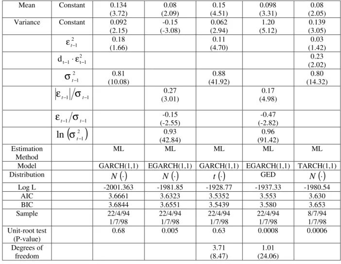
Estimation results for the return of the CBOND are presented in Ta-ble 3. We …nd evidence of asymmetry in the variance for the Gaussian EGARCH (1; 1), theGED EGARCH (1; 1), and theGaussian TARCH (1; 1). All indicate the presence of the leverage e¤ect. As suspected from earlier tests, the distribution of the returns has fat tails: the estimated degrees of freedom for the Student-t GARCH (1; 1) and the GED EGARCH (1; 1) are 3.71 and 1.01 respectively. The latter is statistically di¤erent from two in hy-pothesis testing, corroborating our previous …nding of leptokurtosis. If the asymmetric e¤ect is not taken into account the unit-root test rejects the null, but the opposite happens when it is considered. We conclude that there is evidence of asymmetry, favoring the leverage e¤ect, heavy tails for the con-ditional distribution, and no clear sign of a unit root for the concon-ditional variance.

For the return on COCOA we …nd no asymmetry at all, some evidence of a unit root for the conditional variance, and fat tails; see results in Table 4. The estimated degrees of freedom for the Student-t and GED distributions are respectively 3.32 and 0.977. The latter rejects Normality with high con-…dence in hypothesis testing. It is also interesting to note that, regardless of the distribution used, unit-root evidence is not present when we use the 12_{Using the Generalized Error Distribution allows a Normality test as discussed above.}

At usual levels, conditional Normality is rejected for the return on the US$.

13_{Indeed, average daily returns on the US$ were -0.07% during the wide target-zone}

EGARCH (1; 1) model.

For the return on TELEBRAS we de…nitely …nd asymmetry, favoring the leverage e¤ect; see the results in Table 5. This happens regardless of the model or distribution used. There is also a weak sign of a unit root, again rejected whenever asymmetry is considered. Evidence of fat tails is weaker than that for other series, since the estimated degrees of freedom for the Student-t and GED distribution are respectively 6.81 and 1.41. However, formal statistical testing rejected the Normal distribution again when the GED speci…cation is used.

We now turn to SWARCH -model estimation. First, we entertained the two-regime model, with st = 1 for the low-variance regime, with g1

normal-ized to unity, and with st = 2 when the variance is g2 greater than that in

regimeone. Tables 6 through 9 present estimates using theSWARCH model for all four series. Following Hamilton and Susmel(1994), we considered only the case of Student-t and Normal densities.

For the return of the US$, including a …rst-order autoregressive term for the return did not improve estimation results at all. For the Gaussian SW ARCH (2; 2) model, the t -test for the signi…cance of the AR(1) coef-…cient yields a statistic of 0.6714_{, not signi…cant at usual levels}15_{. There}

is no evidence of asymmetry in the variance either - the t -statistic for the leverage coe¢ cient is virtually zero. Overall, our preferred model is the SWARCH (2; 4), whereas using a Student-t density yields a much higher maximized likelihood value than using the Normal, at the cost of just one more degree of freedom. Indeed, the likelihood-ratio test statistic for com-paring the Student-t density with the Normal for the SWARCH (2; 4) model is ¡ 2 £ (904:39 ¡ 968:72) = 128:66, overwhelmingly signi…cant at any rea-sonable level. Finally, the preferred model for the return on the US$ has a variance in regime two 132.01 times higher than that in the low-variance regime (regime 1).

14_{When the Student-t SW ARCH (2; 2) or t he Gaussian SW ARCH (2; 4) models were}

considered, there were problems …tting a …rst-order autoregression for the mean return, since in all attempt s the value of the likelihood could not beat that of the constant return speci…cation; see Table 6. Even when t he estimation algorithm converged, the t -t est was insigni…cant for the lagged return. We take t hese result as evidence t hat , when the two regimes are considered, there is no …rst -order autocorrelation for the US$ return.

15_{Consistent with the suggestion in Perron(1989) and Hamilton and Susmel(1994) of an}

When the Student-t density was used, the estimated transition probabil-ity matrix was most of the time in the boundary of its constraint. The same is reported for some estimates in Hamilton and Susmel(1994, footnote 5). To avoid meaningless probability estimates, the model was reparameterized to ensure that 0 pi j 1, and

P _k

j = 1pi j = 1. Since calculating the respective

pi j-estimate standard errors is time consuming, we refrain from doing it here.

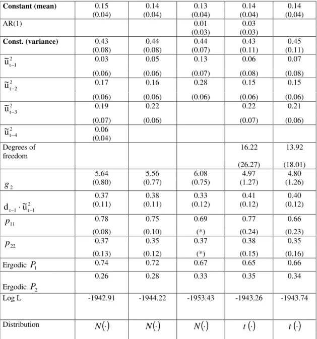
For the return on the CBOND our preferred models is the SWARCH ¡ L (2; 3); notice that the coe¢ cient of the fourth lagged squared error is not signi…cant. Conforming to our previous evidence, the leverage e¤ect for the CBOND is con…rmed using a t -ratio test: 3.45 and 3.33 when using the Student-t and Normal densities respectively. Also based on a t -test, including a …rst-order autoregressive term for the return is insigni…cant, with a t -ratio of 1. When testing which density to use, the likelihood-ratio test statistic for comparing the Student-t density with the Normal for the SWARCH ¡ L (2; 3) model is ¡ 2 £ [¡ 1944:22 ¡ (¡ 1943:74)] = 0:96, which is not signi…cant at usual levels. Thus, it makes little di¤erence which one is chosen here. Given our estimate of g2, CBOND volatility in regime 2 is

about 2.2 times higher than that of regime 1; notice that g2 is statistically

di¤erent than one at usual levels.

For the return on COCOA our preferred models were the Gaussian SW ARCH (2; 4) and the Student-t SWARCH (2; 1)16_{. Con…rming our}

pre-vious results, there is no asymmetry in the variance; a t -ratio smaller than 1 for the leverage coe¢ cient. As it happened for the return of the US$, the estimated transition probability matrix was most of the time in the bound-ary of its constraints when the Student-t density was used, which lead to the estimation of a reparameterized model for which we do not report standard errors for probability estimates. Last, when we compared the Student-t with the Normal for the SWARCH (2; 4), the likelihood-ratio test statistic was ¡ 2 £ [¡ 3968:02 ¡ (¡ 3912:25)] = 111:54, which overwhelmingly signi…cant at usual levels. Therefore it seems more appropriate to use the Student-t distribution17_{. Given our estimate of g}

2 for the Student-t SWARCH (2; 1),

16_{Using a St udent-t density proved to bedi¢ cult in estimation, sincewehad convergence}

problems in several occasions. In particular, we could not …t a SW ARCH (2; 2) model, a candidate for a parsimonious alternative to the SW ARCH (2; 4). Although there were no convergence problems for the St udent-t SW ARCH (2; 1) (see Table 8), it would be interesting to compare it with the SW ARCH (2; 2).

17_{A major di¤erence in Student-t- and Gaussian-density estimates is for the transition}

COCOA volatility in regime 2 is about 1.7 times higher than that of regime 1; notice that g2 is statistically di¤erent than one at usual levels.

For the return on TELEBRAS our preferred models is the SWARCH ¡ L (2; 4). Comparing the Student-t to the Normal yields a likelihood-ratio test statistic of ¡ 2 £ [¡ 2484:14 ¡ (¡ 2475:90)] = 16:48, which is signi…cant at usual levels. The key di¤erence between Student-t- and Gaussian-density estimates is in the transition probability-matrix parameters. For the Gaus-sian case, bp11 = 0:44 and bp22 = 0:93, whereas for the Student-t bp11 = 0:99

and bp22 = 0:99. The scale parameter and the volatility constant are also

dif-ferent for the two speci…cations. For the Student-t bg2= 3:50 and b®0= 1:97,

while for the Gaussian case bg2= 22:75 and b®0= 0:10. Given our estimate of

g2for the Student-t SW ARCH ¡ L (2; 4), TELEBRAS volatility in regime 2

is about 1.9 times higher than that of regime 1; notice that g2is statistically

di¤erent than one at usual levels. Conforming to our previous evidence, the leverage e¤ect is present and signi…cant for all estimated models. For our preferred model, the leverage coe¢ cient is 0.30, with a t -ratio of 3.33.

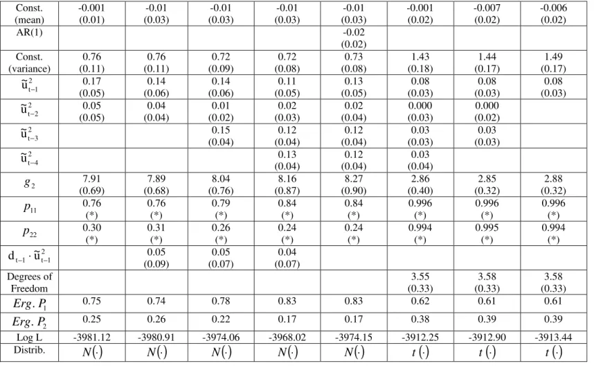
A last modelling e¤ort is made using SWARCH models, in which a three-regime model is entertained. Following Hamilton and Susmel the goal is to allow for an extra regime to capture extreme outliers in the data set; see their discussion in pp. 327-330. This may be useful for Brazilian data since the chances of observing outliers here are much higher than those in developed economies. Estimates using the Gaussian density are reported for the returns of the US$, the CBOND, and TELEBRAS in Table 10. Due to convergence problems, neither returns on COCOA could be estimated using a Gaussian speci…cation, nor could be returns on any of the assets using the Student-t density.

Following our previous results, the returns on the CBOND and TELE-BRAS allow for the leverage e¤ect. To make numerical estimation feasible, The order of the ARCH models had to be limited to two18_{, which resulted}

in a SWARCH ¡ L (3; 2) model for the returns on the CBOND and TELE-BRAS, and a SWARCH (3; 2) model for the return on COCOA. The three-regime models were tested against their two-three-regime counterparts using the likelihood-ratio test statistic19_{. Thelatter is¡ 2£ [883:07 ¡ (909:67)] = 53:20,}

Student-t bp11= 0:996 and bp22= 0:994.

18_{The GAUSS code uses the OPTMUM library. Due to memory rest rictions of our}

current version of GAUSS (3.2), even when the memory ext ension command was present, it was infeasible t o allow for ARCH models wit h order higher than two.

¡ 2£ [¡ 1953:42 ¡ (¡ 1946:38)] = 14:08, and ¡ 2£ [¡ 2485:63 ¡ (¡ 2482:63)] = 6:00, for their return on the US$, on the CBOND and on TELEBRAS respec-tively. Under correct speci…cation, these test statistics are asymptotically distributed chi-squared with 3, 2, and 1 degrees of freedom respectively, re-jecting the two-regime models are rejected at 5% signi…cance.

4.3 Compar ing D i¤er ent ARCH -M odel Est im at es

This Section focus on comparing goodness-of-…t and forecasting accuracy for ARCH -models. The goodness-of-…t statistics used here are all likelihood based. In particular, we consider the maximum of the log-likelihood function, and the Akaike(1973) and Schwarz(1978) information criteria, which are a function of the former. Comparing forecasting accuracy of di¤erent models that predict theconditional mean of a given variableisa simpletask. Suppose that we have the sequence f yt; xtgT + N_{t= 1} of realizations of random variables,

where yt is the realization of the explained variable in a regression, and xt

is a vector containing realizations of possible explanatory variables for yt. In

principle, we could consider M di¤erent models, indexed by i = 1; ¢¢¢M , that hold for the population counterparts of yt; xt with error "it:

Yt = fi(Xt; ¯i) + "it; (30)

where t = 1; ¢¢¢T. Based on some optimality criteria, these M models could be estimated, resulting in b¯_i - model i ’s estimate for the conditional-mean parameter ¯_i. Conditional on xt, for t = T + 1; ¢¢¢N , the out-of-sample

forecasting accuracy of these M models could be compared using some loss-function. In particular, if the mean-squared-error function is considered, the following statistic for all M models could be calculated:

M SEi _{= N}¡ 1 XN t= T + 1

³

yt ¡ fi

³ xt; b¯ i

´ ´₂ ;

i = 1; ¢¢¢M : (31)

Under the usual caveats, the “ best” model would be the one with the smallest value for (31).

Unfortunately, this same procedure cannot be replicated if the goal is to measure forecasting accuracy for the conditional variance (the same applies to volatility). This happens because the conditional variance is not a ran-dom variable for which we can collect realizations to form statistics such as (31). On the contrary, ¾2

t is an unknown time-varying parameter that could,

at best, be estimated consistently when the true Data Generating Process (DGP) is known. In general, since the DGP is unknown, there is no hope of even getting a consistent estimate.

Recognizing this problem, di¤erent authors have proposed tracking down not the conditional variance but some other variable, which may be the same for all volatility forecasts. For example, Heynen and Kat(1994) use what they label “ realized volatility,” a degrees-of-freedom corrected ver-sion of (27). Others have proposed using implicit volatility; see Engle and Mustafa(1992). On the other hand, using the de…nition of conditional vari-ance, i.e., ¾2

t = E ["2t j - t¡ 1], Hamilton and Susmel propose comparing each

model’s variance forecast with what it is supposed to track down. Think-ing in terms of one-step-ahead forecast errors, they propose comparThink-ing ¾2 t

with "2

t, using their respective estimates. We follow Hamilton and Susmel in

assessing the forecast accuracy of our volatility estimates by using four di¤er-ent lossfunctions: mean-squared-error (M SE), mean-absolute-error (M AE), mean-squared-log-error [LE]2, and mean-absolute-log-error jLEj. Results are presented in Tables 11 through 14.

For the return of the US$, the EGARCH (1; 1) performs very well. For the[LE]2and jLEj lossfunctions, thebest model istheGaussian EGARCH (1; 1). When the M AE is used the GED EGARCH (1; 1) is the best, followed closely by the Gaussian SWARCH (3; 2), which is the best when the M SE is used.

For thereturn on the CBOND, the GARCH (1; 1) using either a Gaussian or Student-t speci…cation performs best for the[LE]2and jLEj functions. For the M AE or the M SE functions the Gaussian EGARCH (1; 1) is the best model. It is worth mentioning that the Gaussian SWARCH (3; 2) does also well when we used the M SE, the M AE, and the jLEj functions.

used the [LE]2and the jLEj functions.

For the return on TELEBRAS, the Gaussian GARCH (1; 1) performs best for the [LE]2and jLE j functions. For the M AE function, the Gaussian EGARCH (1; 1) is the best model, but for the M SE function, the Gaussian TARCH (1; 1) is the best model.

Overall, the Gaussian EGARCH (1; 1) performed very well. Similar re-sults are obtained by Pagan and Schwert(1990) and Engle and Ng(1991). Since for the EGARCH model the impact of squared errors on the con-ditional variance is exponential, it is thought to react too much to lagged standardized errors. This may be bad if large errors are infrequent, with the model over-predicting the variance in response to a sequence of small errors. However, if large errors are common, this feature may not be bad, since it also matters how well the model forecast outliers.

The forecasting performance SWARCH models was not encouraging compared to other models of the ARCH class. Hamilton and Susmel criticize standard GARCH models for overestimating the persistence of volatility20_.

Indeed, they write in p. 316 that “ Engle and Mustafa(1992) concluded on the basis of stock option prices that the volatility consequences of the 1987 crash disappeared more rapidly than is suggested by the ... [behavior of the Student-t TARCH (1; 1) model]. Lamoureux and Lastrapes(1993) pre-sented related evidence based on earlier data that standard GARCH models overforecast the persistence in volatility.” If this is true, our forecasting re-sults show that overforecasting actually helped ARCH models that neglect regime switching. This may be related to the frequency and size of outliers for Brazilian data. If outliers are rare, it is probably not very good to have a model which frequently overestimates the volatility of regular standardized errors. However, if outliers are frequent, overforecasting will hurt the forecast of mid-sized errors but probably bene…t the forecast of outliers. Since these make a large contribution to the average forecasting error, the net result may be favorable to models with this feature. Despite this conjecture, It is worth noting that for the return on the US$, where there are clearly distinct regimes, the Gaussian SWARCH (3; 2) performed well, as expected.

Finally, we present goodness-of-…t statistics for most regressions in Ta-bles 15 through 18. For the return on the US$ and on TELEBRAS, the best

20_{For t he value-weighted portfolio of the NYSE, Hamilt on and Susmel …nd the}

model is the Student-t SWARCH (2; 4), although for TELEBRAS, using the Schwarz criterium, one would have chosen the Student-t GARCH (1; 1), be-cause the former has too many parameters. For the return on the CBOND the best model is the Student-t GARCH (1; 1), and for the return on the COCOA the best is the GED EGARCH (1; 1). These results partially reha-bilitatemodelsin theSWARCH class, although it deserves further investiga-tion why their forecasting performance is not as good as their goodness-of-…t statistics.

5 Conclusions and Fur t her Resear ch

The goal of this paper was to present a comprehensive empirical analysis of the return and conditional variance of four Brazilian …nancial series using models of the ARCH class. To discuss the empirical results in greater depth, a self-contained theoretical Section presents ARCH models in a way that it is useful for the applied researcher. References to complete surveys are also given.

The empirical results show a distinct behavior for these four …nancial se-ries. Although all series share ARCH and are leptokurtic relative to the Nor-mal, the return on the US$ has clearly regime switching and no asymmetry for the variance, the return on COCOA has no asymmetry, while the returns on the CBOND and TELEBRAS have clear signs of asymmetry favoring the leverage e¤ect. All these stylized facts were modelled using the ARCH class. Regarding forecasting, the best model overall was the EGARCH (1; 1), in its Gaussian version. Di¤erent versions of the GARCH (1; 1) also performed well, while the SWARCH only did well for the return on the US$, which has a distinct pattern of regimes for the sample period. Regarding goodness-of-…t statistics, the SWARCH model did well, followed closely by the Student-t GARCH (1; 1).

Refer ences

[1] Akaike, H. (1973) Information Theory and an Extension of the Maxi-mum Likelihood Principle, in: B.N. Petrov and F. Csáki, eds., Second International Symposium on Information Theory. Akadémiai Kiadó: Bu-dapest.

[2] Black, F. (1976) Studies of Stock Price Volatility Changes, Proceed-ings from the American Statistical Association, Business and Economic Statistics Section, 177-181.

[3] Black, F. and M.Scholes (1973) The Pricing of Options and Corporate Liabilities, Journal of Political Economy, 81, 637-659.

[4] Bollerslev, Tim (1986). Generalized Autoregressive Conditional Het-eroskedasticity, Journal of Econometrics 31, 307-327.

[5] Bollerslev, T. (1987) A Conditional Heteroskedastic Time Series Model for Speculative Prices and Rates of Return, Review of Economics and Statistics, 69, 542-547.

[6] Bollerslev Tim, Ray Y. Chou, and Kenneth F. Kroner (1992) ARCH Modeling in Finance: A Review of the Theory and Empirical Evidence, Journal of Econometrics 52, 559.

[7] Bollerslev, Tim and Je¤rey M. Wooldridge(1992) Quasi-Maximum Like-lihood Estimation and Inference in Dynamic Models with Time Varying Covariances, Econometric Reviews, 11, 143-172.

[8] Bollerslev, Tim, Robert F. Engle and Daniel B. Nelson (1994) ARCH Models, in Chapter 49 of Handbook of Econometrics, Volume 4, North-Holland.

[9] Box, G.E.P., and G.M. Jenkins (1976) Time Series Analysis: Forecasting and Control. Holden day: San Francisco, CA. Second Edition.

[10] Campbell, J.Y., Lo, A.W., and MacKinlay, A.C. (1997), The Economet-rics of Financial Markets. Princeton: Princeton University Press.

[12] Engle, Robert F. (1982), Autoregressive Conditional Heteroskedasticity with Estimates of the Variance of U.K. In‡ation, Econometrica, 50, 987-1008.

[13] Engle, Robert F. (1983), Estimates of the Variance of U.S. In‡ation Based upon the ARCH Model, Journal of Money, Credit and Banking, 15.

[14] Engle, Robert F. (1995), ARCH: Selected Readings. Oxford: Oxford University Press.

[15] Engle, R.F. and G. Gonzalez-Rivera (1991) Semiparametric ARCH Models, Journal of Business and Economic Statistics, 9, 345-359.

[16] Engle, R.F. and C. Mustafa (1992) Implied ARCH Models from Options Prices, Journal of Econometircs, 52, 289-311.

[17] Engle, Robert F. and Victor K. Ng (1993) Measuring and Testing the Impact of News on Volatility, Journal of Finance, 48, 1022-1082.

[18] Friedman, M. (1977), Nobel Lecture: In‡ation and Unemployment, Journal fo Political Economy, 85.

[19] Gallant, A.R. and G.Tauchen (1989) Semi Non-Parametric Estimation of Cinditionally Constrained Heterogeneous Processes: Asset Pricing Applications, Econometrica, 57, 1091-1120.

[20] Gallant, A.R., D.A. Hsieh and G. Tauchen (1991) On Fitting a Re-calcitrant Series: The Pound/ Dollar Exchange Rate 1974-83, in: W.A. Barnett, J. Powell and G. Tauchen, eds., Nonparametric and Semipara-metric Methods in EconoSemipara-metrics and Statistics. Cambridge University Press: Cambridge.

[21] Gallant, A.R., P.E. Rossi and G. Tauchen (1992) Stock Prices and Vol-ume, Review of Financial Studies, 5, 199-242.

[22] Gallant, A.R., P.E. Rossi and G. Tauchen (1993) Non linear Dynamic Structures, Econometrica, 61, 871-907.

[24] Granger, C.W.J. and Andersen, A. (1978), An Introduction to Bilinear Time-Series Models. Göttingen.

[25] Hamilton, James D. (1994) Time Series Analysis, Princeton University Press.

[26] Hamilton, James D., and Raul Susmel (1994) Autoregressive Condi-tional Heteroskedasticity and Changes in Regime, Journal of Economet-rics, 64, 307-333.

[27] Jarque, C. and Bera, A. (1987), A Test for Normality of Observations and Regression Residuals, International Statistical Review, 55, 163-172.

[28] Lamoureux, Christopher G. and William D. Lastrapes (1990) Persis-tence in Variance, Structural Change and the GARCH model. Journal of Business and Economic Statistics 8, 225-234.

[29] Lamoureux, Christopher G. and William D. Lastrapes (1993) Forecast-ing Stock Return Variance: Toward an UnderstandForecast-ing of Stochastic Im-plied Volatilities, Review of Financial Studies, 5, 293-326.

[30] Mandelbrot, B. (1963) The Variation of Certain Speculative Prices, Journal of Business, 36, 394-419.

[31] Nelson, D.B. (1990) ARCH Models as Di¤usion Aproximations, Journal of Econometrics, 45, 7-38.

[32] Nelson, Daniel B. (1991) Conditional Heteroskedasticity in Asset Re-turns: A New Approach, Econometrica, 59, 347-370.

[33] Newey, Whitney and Kenneth West (1987) A Simple Positive Semi-De…nite, Heteroskedasticity and Autocorrelation Consistent Covariance Matrix, Econometrica, 55, 703-708.

[34] Okun, A. (1971), The Mirage of Steady In‡ation, Brookings Papers on Economic Activity, 2.

[35] Pagan, A.R. and G.W. Schwert (1990) Alternative Models for Condi-tional Stock Volatility, Journal of Econometrics, 45, 267-290.

[37] Schwarz, G. (1978) Estimating the Dimension of a Model. Annals of Statistics, 6, 461-464.

[38] Tauchen, George (1986). Statistical Properties of Generalized Method-of-Moments Estimators of Structural Parameters Obtained From Finan-cial Market Data, Journal of Business & Economic Statistics, 4, 397-416.

[39] Weiss, A.A. (1986) Asymptotic Theory for ARCH Models: Estimation and Testing, Econometric Theory, 2 107-131.

Table 1: Stylized Facts of Brazilian Returns

a) Descriptive Statistics

US$ CBOND COCOA TELEBRAS Mean Daily Return (%) 0.023 0.067 0.032 0.114 Skewness 0.181 -0.545 0.405 0.685 Kurtosis 18.641 17.727 9.483 15.741 Jarque-Bera Test (P-value) 0.000 0.000 0.000 0.000 Unconditional standard deviation 0.282 1.875 1.633 3.227 ARCH(5) Test (P-value) 0.000 0.000 0.000 0.000 AR(1) Robust t-test (P-value) 0.006 0.928 0.200 0.99 Number of Observations 1039 1094 2210 1039 Notes:

(1) AR(1) coefficient standard error calculated using the procedure in Newey and West (1987).

b) Autocorrelation and Partial Autocorrelation Functions of Returns and Squared Returns

Returns US$ CBOND COCOA TELEBRAS

( )

ρ 0.106 (0.106) -0.007 (-0.007) -0.039 (-0.039) -0.002 (-0.002)

( )

ρ -0.012 (-0.023) 0.017 (0.017) -0.042 (-0.044) -0.030 (-0.030)

( )

ρ -0.082 (-0.079) -0.107 (-0.107) -0.007 (-0.010) -0.042 (-0.042)

( )

ρ 0.037 (0.055) -0.013 (-0.015) 0.013 (0.011) -0.025 (-0.026)

( )

ρ 0.120 (0.110) -0.037 (-0.035) -0.010 (-0.010) -0.080 (-0.083)

T

2 0.062 0.060 0.043 0.062

Squared Returns US$ CBOND COCOA TELEBRAS

( )

ρ 0.234 (0.234) 0.271 (0.271) 0.123 (0.123) 0.145 (0.145)

( )

ρ 0.157 (0.108) 0.287 (0.230) 0.042 (0.027) 0.217 (0.200)

( )

ρ 0.160 (0.109) 0.234 (0.128) 0.028(0.020) 0.154 (0.106)

( )

ρ 0.160 (0.097) 0.060 (-0.087) 0.017 (0.010) 0.084 (0.014)

( )

ρ 0.162 (0.091) 0.074 (-0.008) 0.058 (0.055) 0.105 (0.047)

T

2 0.062 0.060 0.043 0.062

Notes:

Table 2: Basic ARCH Estimates for the Return on the US$

Mean Constant 0.028 (13.41) 0.031 (9.03) 0.024 (15.73) 0.019 (18.13) 0.029 (14.42) Variance Constant 9.96.E-5

(1.51) -0.32 (-3.98) 0.0002 (2.72) 166.91 (0.02) 8.38E-5 (1.40) 2 1 − t ε 0.22 (3.37) 0.28 (3.37) 0.30 (3.89) 2 1 t 1 t

d₋ ⋅ε₋ -0.18

(-1.76) 2 1 − t

σ

σ

ε

σ

ε

( )

1

ln

σ

0.99 (126.41) 0.999 (443.99) Estimation Method

ML ML ML ML ML

Model GARCH(1,1) EGARCH(1,1) GARCH (1,1) EGARCH (1,1) TARCH(1,1) Distribution _N

( )

( )

( )

( )

Log L 872.31 876.79 945.66 931.75 882.56 AIC -1.6714 -1.6781 -1.8107 -1.782 -1.689 BIC -1.6524 -1.6543 -1.7869 -1.753 -1.665 Sample 8/7/94 1/7/98 8/7/94 1/7/98 8/7/94 1/7/98 8/7/94 1/7/94 8/7/94 1.7/98 Unit-root test (P-value)

0.35 0.45 0.17 0.98 0.047 Degrees of freedom 2.64 (10.82) 0.82 (22.25) Notes:

(1) t-statistics in parentheses.

(2) Gaussian EGARCH(1,1) estimates equation (15), while EGARCH(1,1) with the GED specification estimates equation (16).

Table 3: Basic ARCH Estimates for the Return on the CBOND

Mean Constant 0.134 (3.72) 0.08 (2.09) 0.15 (4.51) 0.098 (3.31) 0.08 (2.05) Variance Constant 0.092

(2.15) -0.15 (-3.08) 0.062 (2.94) 1.20 (5.12) 0.139 (3.05) 2 1 − t ε 0.18 (1.66) 0.11 (4.70) 0.03 (1.42) 2 1 t 1 t

d₋ ⋅ε₋ 0.23

(2.02) 2 1 − t

σ

σ

ε

σ

ε

( )

1

ln

σ

0.96 (91.42) Estimation

Method

ML ML ML ML ML

Model GARCH(1,1) EGARCH(1,1) GARCH(1,1) EGARCH(1,1) TARCH(1,1) Distribution _N

( )

( )

( )

( )

Log L -2001.363 -1981.85 -1928.77 -1937.33 -1980.54 AIC 3.6661 3.6323 3.5352 3.553 3.630 BIC 3.6844 3.6551 3.5439 3.580 3.653 Sample 22/4/94 1/7/98 22/4/94 1/7/98 22/4/94 1/7/98 22/4/94 1/7/98 8/7/94 1/7/98 Unit-root test (P-value)

0.68 0.005 0.63 0.0008 0.0006 Degrees of freedom 3.71 (8.47) 1.01 (24.06) Notes:

(1) t-statistics in parentheses.

(2) Gaussian EGARCH(1,1) estimates equation (15), while EGARCH(1,1) with the GED specification estimates equation (16).

Table 4: Basic ARCH Estimates for the Return on COCOA

Mean Constant 0.029 (0.94) 0.065 (1.94) -0.014 (-0.57) 0.000 (0.000) 0.037 (1.19) Variance Constant 0.017

(2.03) -0.050 (-311) 0.036 (3.35) -5.68 (-1.70) 0.016 (2.03) 2 1 − t ε 0.03 (3.99) 0.04 (4.55) 0.04 (2.03) 2 1 t 1 t

d₋ ⋅ε₋ -0.01

(-0.80) 2 1 − t

σ

σ

ε

σ

ε

( )

1

ln

σ

0.993 (247.04) 0.995 (364.97) Estimation Method

ML ML ML ML ML

Model GARCH(1,1) EGARCH(1,1) GARCH (1,1) EGARCH(1,1) TARCH(1,1) Distribution _N

( )

( )

( )

( )

Log L -4078.65 -4090.70 -3910.23 -3889.42 -4077.27 AIC 3.6947 3.7065 3.5432 3.519 3.694 BIC 3.7050 3.7194 3.5561 3.534 3.707 Sample 11/10/90 1/7/98 11/10/90 1/7/98 11/10/90 1/7/98 5/1/90 1/7/98 8/7/94 1/7/98 Unit-root test (P-value)

0.20 0.07 0.30 0.08 0.9119 Degrees of freedom 3.32 (11.61) 0.977 (30.13) Notes:

(1) t-statistics in parentheses.

(2) Gaussian EGARCH(1,1) estimates equation (15), while EGARCH(1,1) with the GED specification estimates equation (16).

(3) Gaussian GARCH(1,1), TARCH(1,1) and EGARCH(1,1) estimates use the Bollerslev and Wooldridge(1992) quasi-maximum likelihood asymptotic variance-covariance matrix.

Table 5: Basic ARCH Estimates for the Return on TELEBRAS

Mean Constant 0.28 (4.28) 0.18 (2.55) 0.28 (4.02) 0.156 (2.22) 0.177 (2.53) Variance Constant 0.35

(3.23) -0.07 (-1.87) 0.33 (3.24) 2.10 (14.19) 0.52 (3.99) 2 1 − t ε 0.18 (3.97) 0.19 (5.64) 0.04 (1.45) 2 1 t 1 t

d₋ ⋅ε₋ 0.22

(3.40) 2 1 − t

σ

σ

ε

σ

ε

( )

1

ln

σ

0.93 (51.10) 0.93 (5957) Estimation Method

ML ML ML ML ML

Model GARCH(1,1) EGARCH(1,1) GARCH (1,1) EGARCH(1,1) TARCH(1,1) Distribution _N

( )

( )

( )

( )

Log L -2498.84 -2483.38 -2485.67 -2488.63 -2483.45 AIC 4.8178 4.7899 4.7944 4.802 4.79 BIC 4.8368 4.8137 4.8034 4.831 4.81 Sample 8/7/94 1/7/98 8/7/94 1/7/98 8/7/94 1/7/98 8/7/94 1/7/98 8/7/94 1/7/98 Unit-root test (P-value)

0.12 0.000 0.36 0.00003 0.0000 Degrees of freedom 6.81 (4.96) 1.41 (17.52) Notes:

(1) t-statistics in parentheses.

(2) Gaussian EGARCH(1,1) estimates equation (15), while EGARCH(1,1) with the GED specification estimates equation (16).

Table 6: Two-regime SWARCH and SWARCHL Estimates for the Return on the US$

Constant (mean) 0.026 0.026 0.026 0.022 0.022 0.022

(0.002) (0.002) (0.002) (0.002) (0.002) (0.002)

AR(1) 0.02

(0.03)

Const. (variance) 0.001 0.001 0.002 0.003 0.003 0.002

(0.0002) (0.0001) (0.0002) (0.0007) (0.0007) (0.0005)

2 1 t

u ~

− 0.27 0.27 0.30 0.39 0.39 0.35

(0.06) (0.06) (0.08) (0.14) (0.14) (0.11)

2 2 t

u ~

− 0.19 0.20 0.21 0.26 0.26 0.17

(0.05) (0.05) (0.06) (0.11) (0.11) (0.08)

2 3 t

u ~

− 0.08 0.08 0.01 0.000

(0.04) (0.04) (0.03) (0.05)

2 4 t

u ~

− 0.18 0.17 0.15

(0.05) (0.05) (0.07)

Degrees of freedom

2.77 2.78 3.02 (0.30) (0.30) (0.35)

2

g 98.23 98.84 106.77 130.75 130.36 132.01

(18.12) (18.04) (15.60) (24.91) (25.02) (26.80)

2 1 t 1 t ~u

d₋ ⋅ ₋

11

p 0.99 0.989 0.983 0.999 0.999 0.999

(0.005) (*) (*) (*) (*) (*)

22

p 0.97 0.973 0.959 0.998 0.999 0.999

(0.011) (*) (*) (*) (*) (*)

1 . P Erg 2 . P Erg 0.71 0.29 0.71 0.29 0.71 0.29 0.64 0.36 0.64 0.36 0.63 0.37 Log L 904.39 897.32 883.07 961.62 961.64 968.72 Distribution _N

( )

( )

( )

( )

( )

( )

Notes:

(1) Standard Errors in parentheses.